www.nonlin-processes-geophys.net/18/147/2011/ doi:10.5194/npg-18-147-2011
© Author(s) 2011. CC Attribution 3.0 License.
in Geophysics
Post-processing through linear regression
B. Van Schaeybroeck and S. Vannitsem
Koninklijk Meteorologisch Instituut (KMI), Ringlaan 3, 1180 Brussels, Belgium
Received: 23 July 2010 – Revised: 15 December 2010 – Accepted: 8 February 2011 – Published: 7 March 2011
Abstract. Various post-processing techniques are com-pared for both deterministic and ensemble forecasts, all based on linear regression between forecast data and ob-servations. In order to evaluate the quality of the regres-sion methods, three criteria are proposed, related to the ef-fective correction of forecast error, the optimal variability of the corrected forecast and multicollinearity. The regres-sion schemes under consideration include the ordinary least-square (OLS) method, a new time-dependent Tikhonov reg-ularization (TDTR) method, the total least-square method, a new geometric-mean regression (GM), a recently intro-duced error-in-variables (EVMOS) method and, finally, a “best member” OLS method. The advantages and drawbacks of each method are clarified.
These techniques are applied in the context of the 63 Lorenz system, whose model version is affected by both ini-tial condition and model errors. For short forecast lead times, the number and choice of predictors plays an important role. Contrarily to the other techniques, GM degrades when the number of predictors increases. At intermediate lead times, linear regression is unable to provide corrections to the fore-cast and can sometimes degrade the performance (GM and the best member OLS with noise). At long lead times the re-gression schemes (EVMOS, TDTR) which yield the correct variability and the largest correlation between ensemble er-ror and spread, should be preferred.
1 Introduction
Meteorological ensemble prediction systems provide not only a forecast, but also an estimate of its uncertainty. The ensembles are known to display some deficiencies
Correspondence to:
B. Van Schaeybroeck ([email protected])
(Leutbecher and Palmer, 2008) which can be partially cor-rected through post-processing. Such post-processing con-sists of two steps. Firstly, regression is built between fore-cast and measurement, available during a certain training pe-riod, and secondly, the regression is applied to new forecasts. Regression methods are also of primary importance in the rapidly evolving research field concerning the combination of short-term multi-model climate forecasts (Van den Dool, 2006).
The classical linear regression approach of ensemble re-gression is based on ordinary least-square (OLS) fitting. This approach has some weaknesses which can be detrimental in the context of ensemble forecasts. In the present work, it is shown that other linear regression schemes exist which over-come them. One of the well-known problems with the clas-sical linear regression approach is the fact that the corrected forecast converges to the climatological mean for long lead times (Wilks, 2006). Classical linear regression, therefore, fails to reproduce the natural variability caused by a progres-sive decrease of correlations between the true trajectory and the forecast data. To overcome this decrease of forecast vari-ance, a few alternatives were already introduced. First of all, Unger et al. (2009), in an effort to prolong the correlation time, take a “best member” approach and average over the ensemble of forecasts to obtain the OLS regression param-eters. In addition, they compensate the lack of climatologi-cal variability by a kernel method which consists in adding Gaussian noise, an approach also used by Glahn et al. (2009). In Vannitsem (2009), a new regression scheme was proposed which accounts for the presence of both the observational er-rors and the forecast erer-rors. This approach which gives the correct variability at all lead times was tested against the non-homogeneous Gaussian regression using re-forecast data of ECMWF (Vannitsem and Hagedorn, 2011) and found to have good skill.
introduce two new regression schemes: a time-dependent generalized Tikhonov regularization method (TDTR) and a geometric-mean regression, analogous to the one presented in Draper and Yang (1997). Other schemes under considera-tion include the ordinary least-square method (OLS), the to-tal least-square (TLS, Van Huffel and Vandewalle, 1991), the “best member”-OLS method (Unger et al., 2009) and the EV-MOS method, recently proposed by Vannitsem (2009). The latter is generalized for an arbitrary number of predictors and to cope with multicollinearity. The comparison is performed based on three criteria: a correct variability, a reduced fore-cast error and the ability to deal with multicollinearity.
The different regression schemes are tested in the con-text of the Lorenz 1963 model, focussing on the validity of the proposed criteria. We introduce both model and initial-condition errors and consider the dynamics of the statistical features of the corrected-forecast errors.
Section 2 details the problems associated with OLS for en-semble forecasting. The different regression approaches are then introduced in Sect. 3a–f and their quality is evaluated in the context of the low-order Lorenz model (1963) in Sect. 4. The ensemble skills are discussed in Sect. 5. Finally the con-clusions are drawn in Sect. 6.
2 Linear regression and criteria
Consider a system for which a series of measurement data are available for a variableX, as well as one or more fore-cast models. When running model(s) multiple times using slightly perturbed initial conditions and starting at different dates, a set of forecasts is produced. The problem is how to optimally combine both past forecast and measurement data such as to extract as much information as possible and to cor-rect future forecasts. We outline here different approaches to achieve this goal using linear regression.
Assume that the forecast data for P variables Vp (p=
1,...,P) is assembled in theN×P matrixV; hereN is the number of ensemble forecasts multiplied by the number of ensemble members. Also consider theN measurement data for the variableXthat are contained in the vectorX. Regres-sion consists now of finding a solution for theP regression coefficients contained in the vectorβsuch that:
X≈XC with XC=V β. (1)
Here we call XC the predictand or the corrected forecast
while the variablesVp are the predictors. We take for the
first predictor,V1, the corresponding model observable as-sociated withXandV1 is, therefore, also referred to as the uncorrected forecast. The near equality in Eq. (1) is achieved by minimizing some cost function, yet to be defined (see Sect. 3). Note that without loss of generality, we assume the mean value of all variables to be shifted to zero. Let us
define the error:
εX=X− P X
p=1
ξpβp, (2)
whereξpis the corrected predictor associated withVp. The
valueξpmay be looked upon as the value ofVpafter being
deprived of errors of any sort. We denote the discrepancy betweenξpandVpas follows:
εV ,p=Vp−ξp. (3)
Note that the values ofξpare usually hidden and mostly
in-troduced for optimization purposes. In order to assess the usefulness of regression, three criteria are proposed:
1. The method corrects forecast errors.
2. The method can cope with several highly-correlated predictors which may give rise to multicollinearity. 3. The corrected forecast features the variability of the
ob-servation at all lead times, or, in a weaker form, the cor-rected forecast has the correct variability at long lead times. This condition is necessary in the context of en-semble forecasts in order to get a sufficient spread at long lead times.
2.1 Criterion (i): forecast errors
The corrected forecast should be better than the uncorrected forecastV1in the sense that the mean square error between the observation and the corrected forecast (using infinitely large sample sizes) is lower than or equal to the one of the uncorrected forecast.
2.2 Criterion (ii): multicollinearity
Multicollinearity is often encountered when trying to regress a certain variable using highly correlated predictors. In that case, the regression relation may perform well on the train-ing data, but applied to independent data it will give rise to wild and unrealistic results. In that sense, multicollinearity is a form of overfitting, which here is not a consequence of the abundance of regression parameters. Heuristically, mul-ticollinearity can be understood as follows: if two predictors V1 andV2are the same up to a small noise term, ordinary linear regression may yield a predictand which is very close to the training data. However, since V1 andV2 are nearly identical, several linear combinations ofV1andV2may exist that are close to the measurement data, the closest of which may involve large and, therefore, unrealistic regression co-efficients. Generally, the variances of such estimated coeffi-cients are large and the regression is, thus, very sensitive and unstable with respect to independent data.
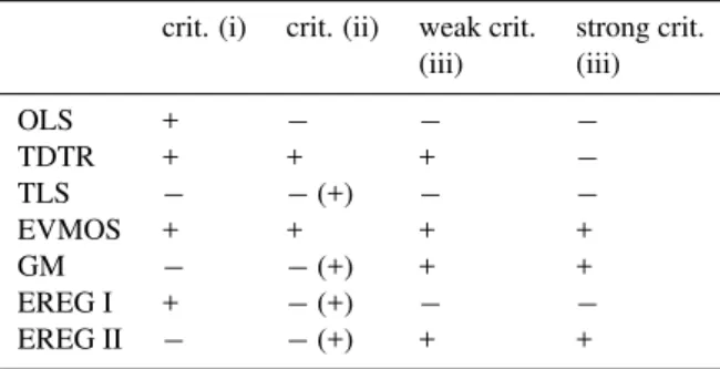
Table 1.Assessment of linear regression methods (rows) based on the criteria (columns) introduced in Sect. 2. A plus sign in brackets means that there exist methods to fulfil this criterion but they are not presented here.
crit. (i) crit. (ii) weak crit. strong crit.
(iii) (iii)
OLS + − − −
TDTR + + + −
TLS − −(+) − −
EVMOS + + + +
GM − −(+) + +
EREG I + −(+) − −
EREG II − −(+) + +
and leave out some variables. Another method consists of eliminating the lowest singular value of the matrix which is to be inverted (as used in principal component regression). A third method is called Tikhonov regularization or ridge re-gression and, from a Bayesian point of view, uses prior in-formation to constrain the regression coefficients.
2.3 Criterion (iii): climatological features at long lead time
It is well known that applying ordinary least-square regres-sion to forecast data amounts to a corrected forecast which converges to the climatological mean for long lead times (Wilks, 2006). This stems from the fact that, due to the chaotic nature of the atmosphere, the correlations between forecast and measurement data irrevocably vanish at long lead time (Vannitsem and Nicolis, 2008). This convergence feature is unrealistic and we can instead try to produce a cor-rected forecast which has a meaningful climatological vari-ability. Such climatological variability is for most systems well known and usually measured as the variance of the available measurement data, σX2. Therefore, criterion (iii) states that, in addition to the correct mean, the variability of a good corrected forecastσXC should equal the climatological variability of the measurement data:
σXC(t )=σX(t ), (4) or at least convergence towards the climatological variability (weaker constraint):
σXC(t )→σX(t ), (5) for long lead times.
Several approaches were already proposed to overcome the lack of variability, including the introduction of an ar-tificial noise term (Unger et al., 2009; Glahn et al., 2009). Let us now introduce the different regression methods com-pared in the present work. We assess their validity using the aforementioned criteria in Table 1.
V
X
{
{
εX XnVn n
EVMOS
n
βε
Σ
2
ε
σ σ
X
X X
n
2 2 2 2
β εVn
C
n +
ξ
Vn n
βξ
n
βV
=
V
X
{
{
εX Xn
Vn n
GM
n
ε
ξ
Vn
n
βV
V
X
{
{
εX Xn
Vn n
TLS
n
ε
=Σε2
Xn
2
εVn
n +
ξ
Vn n
βξ
V
X
{
εX
Vn
OLS
=Σε2 X n
n n Xn
ΣεXnεVn n
=
/2
Fig. 1. Illustration of the cost functionsJ associated with four different regression methods (OLS, TLS, EVMOS and GM) in the case of one predictor. The dots are data points which associate each forecast pointVnto a corresponding measured valueXn. The black line is the regression lineXC=βV.
3 Regression methods
3.1 Ordinary least-square (OLS)
Ordinary least-square (OLS) is the most well-known method of linear fitting. It is implicit in OLS regression that there are no forecast uncertainties, but only measurement errors or, in other words, one assumes thatξp=Vp. The OLS cost
func-tionJOLSis the mean square error of the corrected forecast (see also Fig. 1):
JOLS(β)=DεX2E=D(X−XC)2 E
. (6)
Here h·iis the statistical average over all forecasts. Mini-mization of Eq. (6) with respect toβyields the well-known solution (Casella and Berger, 1990):
βOLS=(VTV)−1VTX. (7)
From Eq. (7) it readily follows that the variance of the cor-rected forecast variable is:
σX2 C= hX
2
Ci = hXXCi. (8)
Therefore, after long lead times, when the correlations
hXVpibetween the observation and the forecast variable
van-ishes, the variance of the predictandXC also vanishes and,
therefore, criterion (iii) is not fulfiled. For the MSE this im-plies:
At long lead times, the MSE is, therefore,σX2.
By construction OLS fulfils the requirement of criterion (i). However, apart from criteria (iii), OLS also fails to sat-isfy (ii) since it cannot cope with multicollinearity, hence, according to our criteria, OLS is not the best method for en-semble regression.
3.2 Time-Dependent Tikhonov Regularization (TDTR) A well-known problem of the OLS regression is that the variance of the regression parameters are very large in case of multicollinearity (Golub and Van Loan, 1996). To over-come this problem, it is the custom to bias the estimates of the regression coefficients using Tikhonov regularization, also called ridge regression. We present here a new time-dependent Tikhonov regularization (TDTR) method for post-processing ensemble forecasts. The generalized TR ap-proach works as follows: instead of minimizingJOLS, a con-straint is added for the values of the regression coefficientsβ
in order to fall within a certain range of a constant valueβ0. More specifically, we demand thatPp(βp−βp0)2is small.
The way to implement such a restriction is by introducing the positive Lagrange multiplierγ (t )(withtbeing time) and minimizing the cost function:
JTDTR(β)=D(X−XC)2 E
+γ (t )X
p
(βp−βp0)2. (10)
The solution is (Bj¨orck, 1996):
βTDTR=VTV+γ (t )I
−1
VTX+γ (t )β0. (11) HereIis the unit matrix. Using this solution, the variability of the corrected forecast is found to be:
σX2
C= hXXCi +γ (t )
X
p
βp(βp0−βp). (12)
For the mean square error, on the other hand, one gets: MSE(TDTR)=σX2− hXXCi −γ (t )
X
p
βp(βp0−βp), (13)
Using these results, a Tikhonov regularization method can be developed in such a way as to fulfil criteria (ii) and the weak criterion (iii) as specified in Sect. 2. From the in-spection of the cost functionJTDTR, it is clear that for large γ the regression coefficient β is forced to converge toβ0. The latter can be chosen in such a way that the corrected forecast has the variability of the measurement data and, thus, satisfies the weak version of criterion (iii). The way to do that is first by Taylor-expanding Eq. (11) up to the first order in 1/γ (t )(with largeγ (t )) which gives a value ofβ≈β0−VTVβ0/γ (t ), which in turn leads to
σXC(t→ ∞)=σX0C and MSE(t→ ∞)=σ 2 X+σX20
C , (14)
whereX0C=Ppβp0Vp. Note that Eqs. (14) are independent
of γ (t ). Now, if the variability of the predictors is known at long lead time (one predictor would suffice in fact), β0
can be chosen in such a way as to satisfy weak criterion (iii): σXC(t→ ∞)=σX.
If we also want a scheme able to cope with multicollinear-ity, or equivalently to fulfil criterion (ii), care must be taken that γ is positive and nonzero but still small at short lead times.
The choice of the time-dependent functionγ (t )is arbitrary but the cross-over time whenγgoes over from being small to being large should preferentially be chosen as a function of the correlations between forecast variables and measurement data. The function used here is:
γ (t )=γ0exp
1 1
|
AC(0)| |AC(t )|−1
. (15)
Hereγ0is a small positive scalar and AC is an anomaly cor-relation AC(t )=PphXVpi/(σXσVp)(Van den Dool, 2006). The constant1is a tolerance percentage of correlation loss in the sense that, if the anomaly correlation AC(t )decreases by an amount1from its value at time zero, the corrected forecast will become strongly biased towards the solution XC0. Note that, at time zero,γ (0)=γ0. We choose in our simulationsγ=10−4 and1=0.5% andβ=βEV (as will be defined later in Eq. (24) for the EVMOS technique).
One may come up with choices for γ different from Eq. (15). For example, we can chooseγ (t )=γ0et /τ where γ0 is again a small positive constant and τ is a constant which characterises the time when the correlations between the forecast and the measurement start to vanish strongly. In the same line, another candidate could be the threshold func-tionγ (t )=γ0+2(t−τ )/γ0with2the Heaviside function. Finally, the new TDTR method fulfils criteria (i), (ii) and weak criterion (iii). Note that it is possible to tune the Tikhonov regularization scheme in such way (by means of γ andβ0) as to fulfil also criterion (iii). However, in that case, one must bias the regression coefficients towards other coefficients on which no information is available, so these must be chosen with some arbitrariness.
3.3 Total least-square (TLS)
The total least-square (TLS) method was introduced as a method to correct OLS to take into account the errors in the forecast model (Golub and Van Loan, 1996). Therefore, the cost function to be minimized is a function of bothεX and
εV of Eqs. (2) and (3) (Van Huffel and Vandewalle, 1991):
JTLS(β,ξ)=
* P
X
p=1
wp2 Vp−ξp2+ X− P X
p=1 ξpβp
!2+ .
(16) Here the weight factorswp are constants which do not
with respect to the variables ξp, one gets a cost function
which only depends on the valuesβp:
JTLS(β)=
(X−XC)2
1+Pp(βp/wp)2
. (17)
After minimization with respect toβp, one gets an exact
so-lution for the regression problem (Van Huffel and Vande-walle, 1991):
β=
VTV−µ2W−2
−1
VTX, (18)
whereµ is the lowest singular value of the composite ma-trix[V;X]andW=diag(w1,...,wP). The variability of the
corrected forecast is then given by:
σX2
C= hXXCi +(σ 2
X− hXXCi) X
p1
(βp1/wp1)
2
!
, (19)
and:
MSE(TLS)= 1+X
p1
(βp1/wp1)
2
!
(σX2− hXXCi). (20)
Two weaknesses of TLS may be pointed out. First, from Eq. (16), it is clear that, since the different predictors may have different physical units, appropriate estimates of the weight factorswp prior to regression are indispensable. A
second weakness of TLS lies in the fact that the regression estimates become meaningless once a predictorVpis
uncor-related with the observationX. For instance, in the case of re-gression with one predictor one finds thatβ∝1/hV Xiwhich diverges as the correlation vanishes. It follows also that TLS can sometimes fail in satisfying criterion (i). Note that meth-ods exist for TLS to deal with multicollinearity (Van Huffel and Vandewalle, 1991). However, we will not address them here. For the numerical analysis in Sect. 4 we takewp=1
for all predictor indicesp. TLS then minimizes the sum of distances between the data points and the regression line (see Fig. 1).
3.4 Error-in-Variable method (EVMOS)
Recently a new regression method, called EVMOS was in-troduced for post-processing ensemble forecasts (Vannitsem, 2009). The cost functionJEVtakes into account the sum of errors in the forecast variablesPpβpεV ,p and the errors in
the measurement variableεX(see Fig. 1 for a visual
interpre-tation):
JEV(β,ξ)= *
XC−Ppξpβp
σXC
!2
+ X−
P pξpβp
σX
!2+ .
(21)
Minimization of Eq. (21) with respect toξpamounts to a cost
function which is a function ofβonly:
JEV(β)=
(X−XC)2
σX2+σX2 C
. (22)
Further minimization yields for each predictor indexp:
X
p1,p2
βp1βp2cXp1cXp2 ρp1p2−2ρpp2
= −σX2. (23)
Hereρp1p2= hVp1Vp2i/(cXp1cXp2)andcXp= hVpXi. This
nonlinear problem has a solution:
βp,EV=
σX
cXp
P p1 ρ
−1 pp1 qP
p1,p2 ρ −1
p2p1
. (24)
The solution for βp for up to two predictors was already
given in Vannitsem (2009). Note that we provide the details of the derivation in Appendix A.
Using now the solution Eq. (24), it is straightforward to derive that the variance of the corrected forecast is exactly the same as the one of the measured data:
σX2 C=σ
2
X. (25)
This equation is valid at all times and, therefore, satisfies cri-terion (iii) (see Eq. (4)). The MSE becomes:
MSE(EV)=2
σX2−σX
s X
p1,p2
ρ−1 p2p1
. (26)
One can also make the EVMOS approach robust against multicollinearity by replacingVp→Vp+ǫpin Eq. (21) with
ǫp a noise term with zero mean and standard deviation γ,
the latter being a small positive constant. After averaging out the noise terms, one arrives at a new cost function which is minimized by the solution:
βp=
σX
cXp
P p1
(ρ+γI)−1pp
1 qP
p1,p2
(ρ+γI)−1 p2p1
. (27)
In practice γ is very small, but still sufficiently large for the variance of the regression coefficients to be sufficiently small. In conclusion, EVMOS is a method which satisfies all proposed criteria.
3.5 Geometric Mean (GM)
The geometric-mean (GM) method with one predictor was introduced by Teisser (1948) and minimizes a cost function which is a sum of triangular areas|εXεV|/2 whereεXandεV
incorporate multiple predictors. Here we introduce a differ-ent approach for such generalization which is still reducible to a weight-free least square problem and satisfies criterion (iii).
The GM approach is introduced in order to overcome one of the main disadvantages of the methods discussed so far which account for both forecast and observation error: for each observation, the associated penalty in the cost function consists of asumof squared errorsεX andεV, normalized
using appropriate weight factors. For TLS these are the con-stantswp and for EVMOS,σX−1andσX−1
C. Therefore, those approaches strongly depend on the weight factors. The GM method with one predictor assists in minimizing the sum of triangular areas where the triangles are formed by connect-ing the fitted line with the measurement point. We extend this approach to more than one predictor by taking the geometric mean of the triangular areas|εXεV ,p|/2 for each predictor
indexp. The GM cost function then becomes:
JGM(β)=
* P
Y
p=1
Vp−ξp
X−
P X
p1=1
ξp1βp1
!
1/P+
. (28)
In order to obtain the value ofξp, a projection into the plane
formed by theX-axis and theVp axis should be performed
such thatξp=(X−Pp16=pVp1βp1)/βp. Substitution leads
us to the least-square expression:
JGM(β)=
(X−XC)2
Qpβp
1/P
. (29)
Minimization of Eq. (29) with respect toβpgives:
−2PβpcXp 1−
X
p1
ρpp1cXp1βp1 !
=D(X−XC)2
E
. (30)
The minimization problem can also be solved by an itera-tive numerical method such as the one explained in the Ap-pendix B.
From Eq. (30), one can derive that the variance of the pre-dictand is the same as the one of the measurement variable: σX2
C=σ 2
X. (31)
As was true for the EVMOS approach, this equation is valid at all times and GM, thus, satisfies criterion (iii). Also, the MSE after optimization satisfies:
MSE=2(σX2− hXXCi). (32)
In case of one predictor, the solution to Eq. (30) yields β=σX/σV which makes it fully equivalent to the EVMOS
approach. Thus, EVMOS with one predictor can be consid-ered the minimization solution to a triangle problem. Note also that, in case of one predictor, the GM problem reduces to the one of Draper and Yang (1997).
10-4
10-5
1 predictor 4 predictors EREG II(1) GM(4) V
MSE
u (t)
2<
r>
10-2 10-1
t
10-3
1
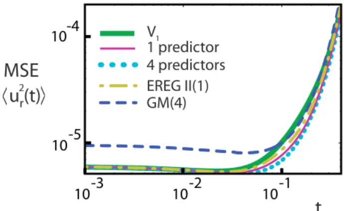
Fig. 2. The short-time mean square error (MSE) evolution for the
Lorenz model with a small model error (δr=2.5×10⁻³) and with 5×10⁵ensembles of 500 members. The lines indicated with “1 predictor” and “4 predictors” apply to all regression methods except for GM and EREG II. The numbers indicated after GM and EREG II are the predictor numbers.
3.6 Best-member regression (EREG I and EREG II) Recently a new approach of ensemble regression was pro-posed by Unger et al. (2009). The authors show that, if all ensemble members are equally apt at being the best, that is, the closest to reality, and, if a linear relationship exists be-tween the best member and the real data, then the regression coefficient of the OLS can be found using the ensemble mean instead of each ensemble member separately.
Consider a measured path of variableX for which mod-elling has resulted in an ensemble of K uncorrected fore-castsV1k(t )(k=1,...,K). The ensemble consists of model runs with the same or different models, starting with slightly different initial conditions. We defineF now as the aver-age over the ensemble members of the uncorrected forecast, or,F=PkV1k/K. In order to calculate the regression co-efficient, we apply OLS usingF instead ofV1as the model predictor. Minimization of the OLS cost function yields: βEREG=
hF Xi
hF2i, (33)
These regression coefficients are then applied to each ensem-ble member to yield the best member or EREG I predictand: XC,I=βEREGV1. (34) From Eq. (33) it is clear that, as is valid for OLS, the vari-ance of the corrected forecast vanishes for long lead times and EREG I will, therefore, not satisfy criterion (iii). How-ever, as was proven in Unger et al. (2009), the damping to-wards zero of this variance is slower than in the case of OLS. In addition, the authors define an EREG II forecastXC,I I
MSE
u (t)
2<
r>
500
250
0
t
10
5
15
V EVMOS(4)
OLS(4)
TDTR(4) EREG I(1) EREG II(1)
GM(4)
1
TLS(4)
Fig. 3. The long lead time mean square error (MSE) evolution for
Lorenz model withsmallmodel error (δr=2.5×10⁻³) and with 5×10⁵ensembles of 500 members. The number after the regression method denotes the predictor number.
varianceσX2−σX2
C,I, satisfying criterion (iii). However, such random noise may destroy physically-relevant statistical in-formation of the error statistics. As will be shown in the next section, at intermediate time-scales EREG II may have a MSE which is larger than the one of the uncorrected fore-cast. Note that the use of more than one predictor can be straightforwardly implemented in the EREG methods as for OLS.
4 Numerical results
We address the usefulness of the different regression meth-ods in the context of a low-order system by focussing on the statistical features of the associated error distributions. We use the well-known Lorenz 1963 model describing thermal convection:
˙
x=σ (−x+y), (35a)
˙
y=rx−y−xz, (35b)
˙
z=xy−bz. (35c)
Here the dot denotes the derivative with respect to time,xis the rate of convective turnover, andyandzquantify the hor-izontal and vertical temperature variation, respectively. The parameter set is fixed to(σ,r,b)=(10,28,8/3)such that the reference system exhibits chaotic behaviour. The model dif-fers from reality by introducing a model error which we take to be the positive biasδrto the (reduced) Rayleigh numberr. For thesmallmodel-error experiment a biasδr=2.5×10⁻³ is introduced while for thelargemodel error experiment a biasδr=10−2is used.
The numerical scheme is integrated using a second-order Runge-Kutta method. An ensemble is constructed by adding at time zero an unbiased Gaussian noise with standard devi-ation 10−3to all variablesx, y andz. In the experiments,
10-3
10-1
10-5
1 predictor 4 predictors EREG II(1) GM(4) V
MSE
u (t)
2<
r>
10 -2
10-1
t
10-3
1
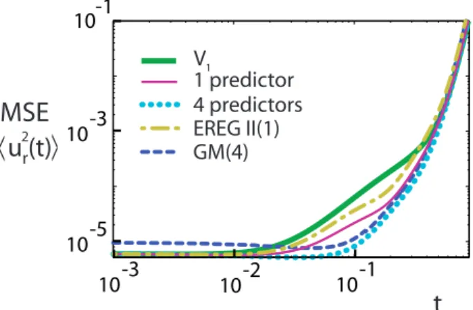
Fig. 4. The short-time mean square error (MSE) evolution for the
Lorenz model withlargemodel error (δr=10−2) and with 5×10⁵ ensembles of 500 members. The lines indicated with “1 predictor” and “4 predictors” apply to all regression methods except for GM and EREG II.
we typically use ensembles of 500 members and averaging is typically done over 50 000 points on the attractor. The train-ing and verification of the regression method is performed using two independent datasets, both of the same size.
Originally ensemble forecasts were mainly designed for medium and long range lead times. Nowadays there is a growing interest in using this technique at shorter time scales to provide uncertainty information for short-range forecast-ing (few hours up to one or two days, Iversen et al., 2010). In the following, we, therefore, present results for the different timescales in order to provide a global picture of the different corrections the post-processing could provide.
We study the errors by probing the statistical properties of one of the following error variables:
ux=x−xC, uy=y−yC, uz=z−zC,and
ur= q
u2
x+u2y+u2z.
Here the indexC refers to the corrected variable. The pre-dictors forxCare the variables(V1,V2,V3,V4)=(x,y,z,yz), generated by different forecasts with model and initial-condition errors and the ones foryCare obtained by
perform-ing the shiftx→y→z→x; applying again this shift gives the predictors forzC. In the plots the number of predictors
are indicated in brackets next to the regression method. 4.1 Small model error
MSE
u (t)
2<
r>
500
250
0
t
10
5
15
V EVMOS(4) TLS(4)
OLS(4)
TDTR(4) EREG I(1) EREG II(1) GM(4)
1
Fig. 5. The mean square error (MSE) evolution for the Lorenz
model withlargemodel error (δr=10−2) for long lead times and with 5×10⁵ensembles of 500 members.
lead times. For all other methods (OLS, TDTR, TLS, EV-MOS and EREG I) the results depend only on the number of predictors used and are, therefore, bundled by the lines “1 predictor” and “4 predictors”. Their resulting MSE is always smaller than the one of the uncorrected forecast and pro-vides a substantial forecast improvement only at the smallest timescales where the number and the choice of predictors are important.
GM with one predictor is exactly the same as EVMOS with one predictor. Hence, if instead of GM(4) we would have used GM(1), the results would be indicated by the “1 predictor”-line in Fig. 2 and, thus, have a lower MSE than GM(4). This suggests that GM is progressively degrading when the number of predictors increases. This behaviour can be explained as follows: assume that we apply GM regres-sion withP −1 predictors and continue by adding a new predictorVP which is totally uncorrelated to all other
pre-dictors and to the observation. Then one expects that the regression coefficientβP associated with this new predictor
equals zero. However, from Eq. (30) it can be shown that βP ∝(2PhVP2i)−1/2. The fact thatβP is generally nonzero
could also be suspected from the cost function (29) which di-verges if a regression coefficient vanishes. Therefore, adding an uncorrelated predictor introduces an instability. Note that higher-order moments of the error distribution are not well corrected at short lead times, whatever the regression tech-nique used.
At the intermediate lead times there is a fast increase of the MSE as a direct consequence of the chaotic nature of the system (Lorenz, 1963). The timescale involved is deter-mined by the inverse of the dominant Lyapunov exponent. At these lead times no improvements with respect to the original forecast variableV1, are achieved by any regression method and the same is true for higher moments of the error distribu-tion. Whereas OLS, TDTR, TLS, EVMOS and EREG I give a MSE equal to the one of the uncorrected forecast, GM(4)
0
-0.008 0 0.008 0.015
0.03
0
t=0.2
t=0.3
-0.01 0 0.01 0.01
0
0.001
0
-0.04 0 0.04
ux
t=1.
0.005 0.01
0
-0.004 0 0.004
t=0.12
ux P(u )x
P(u )x
P(u )x
P(u )x
1 predictor 4 predictors EREG II(1)
V1
1 pr. 4 pr. V1 EREG II(1)
EREG II(1) EREG II(1)
1 predictor 4 predictors
V1 1 predictor
4 predictors V1
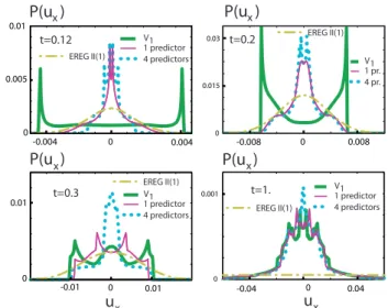
Fig. 6. The distributions of the error variableux of the Lorenz
model with large model error (δr=10−2) andwithoutinitial con-dition error, att=0.12,0.2,0.3,1. The lines indicated with “1 pre-dictor” and “4 predictors” apply to all regression methods except for GM and EREG II. The results are generated using 2×10⁶ en-sembles.
and the EREG II yield a MSE which is larger. Therefore, GM(4) and EREG II are not well-suited for use at intermedi-ate lead times.
Figure 3 shows the evolution of the MSE for long lead times when the errors become large. Large differences be-tween the regression methods are visible. As mentioned before, the MSE of TLS gives unrealistic results once the correlations between the observation X and the predictors vanish. According to weak criterion (iii), the MSE of the EVMOS, TDTR, EREG II and GM(4) forecasts converges to the correct value 2σX2 at long lead times, but before the asymptotic saturation, the MSE of GM(4) and EREG II is still larger than the one of the uncorrected forecast. The MSE of OLS and EREG I, on the other hand, is too low by a factor of two as the variance of the corrected forecast vanishes.
At the intermediate times, a fast increase is present for all moments of the error distribution, giving rise to a power-law error distributionP (uX)for large values of the error such that
P (ux)∝u−xνwith some positive scalarν. Note that a similar
behaviour is also present forP (ur). These power tails are
not affected by the different regression methods.
4.2 Large Model Error
t=0.2
t=0.3 t=1.
0.05
0
0.002
0 0
-0.02 0 0.02 -0.04 0 0.04
t=0.12
uz uz
P(u )z
P(u )z
P(u )z
P(u )z
-0.005 0 0.01
0.02 0.04
0
-0.01 0 0.02
0.002
0.001
1 predictor 4 predictors EREG II(1)
V1
1 predictor 4 predictors EREG II(1)
V1
1 predictor 4 predictors EREG II(1)
V1
1 pred. 4 pred.
EREG II(1)
V1
Fig. 7.The distributions of the error variableuzof the Lorenz model with large model error (δr=10−2) and without initial condition error, att=0.12,0.2,0.3,1. The lines indicated with “1 predictor” and “4 predictors” apply to all regression methods except for GM and EREG II. The results are generated using 2×10⁶ensembles.
As for small model errors the amplitude of the corrections obtained by the post-processing progressively decreases. Moreover, both EREG II and GM(4) yield an even higher MSE than the one of the uncorrected forecast. Note that the increase of model errors expands the interval during which GM(4) effectively corrects the forecast. In Fig. 5, we dis-play the MSE for long lead times. As compared to the case of small model errors, the error saturation now sets in earlier and the result for the EREG I forecast is now closer to the one of OLS.
4.3 Evolution of error distribution
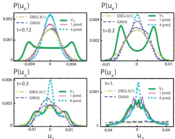
Having looked so far at its second moment, we consider now the evolution of the full error distributions of the original and corrected forecast. In Figs. 6 and 7, the error distribution evolution ofux anduzin the absence of initial condition
er-rors are plotted. As mentioned earlier, for all methods except for EREG II and GM(4) the quality of regression depends almost solely on the number of predictors.
At timet=0.12 the regression distribution forux(Fig. 6)
with one predictor is peaked close to the centre. The double-peak feature of the corrected forecast seems to disappear at t=0.2, but appears back again for longer lead time. With four predictors multiple peaks are still present, but the distri-bution is well centred around zero. At a later time (t=1.), all regressed distributions except for EREG II are close to each other, all featuring a multiple-peak structure. The EREG II distribution is by construction a smoother version of the EREG I distribution (here indicated by “1 predictor”) and
-0.01 0 0.01
t=0.2
t=0.3
-0.01 0 0.01
0.006
0.003
0 0
-0.04 0 0.04
ux
t=1. 0.001
0.002
0
-0.004 0 0.004
t=0.12
ux
P(u )x
P(u )x
P(u )x
P(u )x
0.002 0.004
0.001 1 pred.
4 pred.
EREG II(1) V1
GM(4) 1 pred.
4 pred. V1 EREG II(1)
GM(4)
1 pred. 4 pred. V1 EREG II(1)
GM(4) EREG II(1)
GM(4) 1 pred.
4 pred. V1
Fig. 8. The distributions of the error variableux of the Lorenz
model with small model error (δr=2.5×10⁻³) andwith initial condition errors, att=0.12,0.2,0.3. The lines indicated with “1 predictor” and “4 predictors” apply to all regression methods ex-cept for GM and EREG II. The results are generated using 5×10⁵ ensembles of 500 members.
tends to be Gaussian-like at all lead times. Such broadening leads to a loss of the statistical information contained in the error distribution. At short times EREG II features a smaller MSE than the one of the uncorrected forecast. However, at longer lead times (t >0.2) the broadening of the distribution produces errors with magnitudes larger than the one present in the uncorrected forecast. At timet=1 the error distribu-tion of EREG II is almost flat with much larger values than the uncorrected forecast. Note that similar results are ob-tained for other magnitudes of the model error and for the distributions ofuy.
The probability distributions ofuzin Fig. 7 obtained with
one predictor removes, to a great extent, the systematic bias ofuz. The “4 predictor” case, on the other hand, also reduces
the variance of the error distribution.
Figure 8 displays the results using the same model config-uration butwithinitial-condition errors. It is clear that the sharp peaks present in the uncorrected forecast of Fig. 6 are now strongly smoothed out, but their positions are well pre-served. The double-peak structure of the distributions after regression, however, seems to have disappeared. As a result of the chaotic nature of the system, the error distributions at timet=1 with and without initial condition errors are very much alike.
100
10-2
10 -4
10 -6
10 -6
10 -6 10
-6
MSE F Spread V
MSE EVMOS(4),OLS(4), TLS(4),TDTR(4)
10 -2
10-1 100
t
10-3
1
Spread EVMOS(4),OLS(4), TLS(4),TDTR(4)
100
10-2
10 -4
MSE F Spread V
MSE EVMOS(1), OLS(1), TLS(1), TDTR(1), EREG I (1)
10 -2
10-1 100
t
10-3
1
Spread EVMOS(1),OLS(1), TLS(1), TDTR(1), EREG I(1)
100
10-2
10 -4
MSE F Spread V
MSE EREG II (1)
10 -2
10 -1
10 0
t
10-3
1
Spread EREG II (1) 4 predictors
EREG II
t
100
10-2
10 -4
MSE F Spread V MSE GM(4)
10 -2
10 -1
10 0
t
10-3
1
Spread GM(4) GM (4) 1 predictor
Fig. 9. Ensemble variance (spread) and mean square error of the
ensemble mean of the uncorrected forecastV1 against corrected
forecasts produced by different regression methods as a function of time, generated using the Lorenz model with large model error (δr=10−2) and averaged over 5×10⁵ensembles of 500 members each. Note that the EREG II ensemble variance and mean square error of the ensemble mean are identical.
lead times, due to the large noise variance used to generate the EREG II forecast, the MSE of EREG II is well beyond the uncorrected forecast, leading to an almost flat unrealistic distribution.
5 Ensemble features
As pointed out in the Introduction, the main reason for look-ing at alternative linear post-processlook-ing is to investigate the possibility of post-processingensembleforecasts. One im-portant reason for the use of ensemble forecasts is that it pro-vides one with an estimate of the forecast uncertainty. In this section we explore, using numerical experiments, how the relationship between the ensemble spread and forecast ac-curacy is affected by post-processing. We compare first the average ensemble error with the average ensemble spreads, and we proceed by considering the relation between error and spread of each ensemble separately.
One requirement for a good ensemble forecast is to have a mean square error of the ensemble mean equal to the ensem-ble variance (e.g. Leutbecher and Palmer, 2008). In Fig. 9 the error of the ensemble mean is compared with the ensemble variance. The corresponding quantities for the uncorrected forecast are also displayed using green symbols. Except for EREG II, regression does not affect the ensemble variance of the uncorrected forecast at short lead times. The error dy-namics of the ensemble mean, on the other hand, is similar to the mean square error evolution of all ensemble members as shown in Fig. 4. Note that such regressions give rise to
en-t
EVMOS(4) OLS(4)
EREG II(1) 1
0.1
0.001 0.01 0.1 1
V1
Perfect model
spr
ead-er
ro
r c
o
rr
ela
tion
Fig. 10. Log-log plot of the ensemble spread-error correlation
against time for short time scales. The spread is the square root of the ensemble variance and the error is the ensemble average of ur. The results are generated using the Lorenz model with large model error (δr=10−2) and averaged over 2×10⁵ensembles of 500 members each. The perfect-model result is obtained without model error.
sembles which remain underdispersive except for the EREG II ensemble. Due to the unbiased noise used to construct the EREG II ensemble, the MSE of the ensemble mean of EREG I and EREG II are identical. The gain of ensemble variance without loss of accuracy of the ensemble mean constitutes the most interesting feature of EREG II but it is obtained at the expense of an increase of the overall ensemble member error as shown in Fig. 4 and a broadening of the error distri-bution (e.g. Figs. 6 and 8). In agreement with our previous results, at long lead times when the errors are saturated, the average ensemble variance converges to the error of the en-semble mean for EREG II, EVMOS, TDTR and GM ensem-bles.
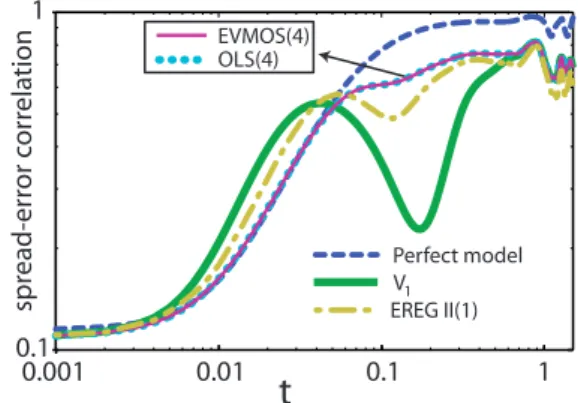
We study now in what sense the ensemble spread can be considered a measure of the actual error and how it is affected by post-processing. Figure 10 shows the Pearson correlation between ensemble spread and ensemble error. The ensem-ble spread refers to the square root of the ensemensem-ble variance and the error is the root-mean-square errorur over all
PERFECT MODEL V : UNCORRECTED FC
EVMOS (4) EREG (1)
0 0.01 0.02 0.03
0.005 0.01 0
0.01 0.02 0.03
0.005 0.01
0 0.01 0.02 0.03
0.005 0.01
0 0.01 0.02 0.03
0.005 0.01
1
SPREAD
SPREAD SPREAD
SPREAD
ERROR ERROR
ERROR ERROR
Fig. 11.Scatterplot of spread against error of 10 000 ensembles at t=0.2. The spread is the square root of the ensemble variance and the error is the ensemble average ofur. The results are generated using the Lorenz model with large model error (δr=10−2) using ensembles of 500 members each. The perfect-model result is ob-tained without model error.
the correlation. We illustrate this in Fig. 11 with scatterplots of spread against error for 10 000 ensembles att=0.2. The strong spread-error correlation for the perfect model is obvi-ous from a clustering of dots along the diagonal. On the con-trary, the imperfect-model ensembles are strongly dispersed. The post-processing procedures are capable of strongly re-ducing the errors such that a great deal of spread-error cor-relation is recovered. Note that the addition of random noise of the EREG II method amounts to a shift of the ensemble cloud along the diagonal.
The correlations at intermediate and long timescales are plotted in Fig. 12. At intermediate timescales the spread-error correlation is large as the standard deviation of ensem-ble spread is now on average ten times larger than the average ensemble spread. Even though the spread-error correlation of the uncorrected and the EVMOS ensembles are approx-imately equal to the one of EREG II, the associated errors and spreads strongly differ. This is illustrated in Fig. 13 by scatterplots att=2. The uncorrected and EVMOS ensem-ble clouds are much alike but the EREG II cloud is shifted along the diagonal, a transformation which preserves the lin-ear correlation. Note also the enlarged scale of the EREG II plot. Finally, due to the error saturation, a progressive cor-relation decrease sets in for all ensembles at lead timest=5 (see Fig. 12). Remarkably, the OLS and EREG II correla-tions are distinctly smaller than the ones of the uncorrected and EVMOS ensembles. Att=15, the variance of ensemble spread for all except the EREG II ensembles is still signifi-cant as suggested in Fig. 14.
t
EVMOS(4) OLS(4) EREG II(1)
1
0.5
0 10 20
V1
Perfect model
spr
ead-er
ro
r c
o
rr
ela
tion
Fig. 12. The spread-error correlation against time for
intermedi-ate and long times. The spread is the square root of the ensem-ble variance and the error is the ensemensem-ble average ofur. The re-sults are generated using the Lorenz model with large model error (δr=10−2) and averaged over 2×10⁵ensembles of 500 members each.
PERFECT MODEL V : UNCORRECTED FC
EVMOS (4) EREG II (1)
SPREAD
SPREAD SPREAD
SPREAD
ERROR ERROR
ERROR ERROR
0 0.5 1
0.5 1
0 0.5 1
0.5 1
0 0.5 1
0.5 1
0 1 2
1 2
1
Fig. 13.Scatterplot of spread against error of 10 000 ensembles at t=2. The spread is the square root of the ensemble variance and the error is the ensemble average ofur. The results are generated using the Lorenz model with large model error (δr=10−2) using ensem-bles of 500 members each. The perfect-model result is obtained without model error. Note the scale of the EREG II plot which has a scale which is twice as large.
PERFECT MODEL V : UNCORRECTED FC
EVMOS (4) EREG II (1)
10
0 6 12
20
30 1
10
0 6 12
20 30
10
0 6 12
20 30
10
0 6 12
20 30 SPREAD
SPREAD SPREAD
SPREAD
ERROR ERROR
ERROR ERROR
Fig. 14.Scatterplot of spread against error of 10 000 ensembles at t=15. The spread is the square root of the ensemble variance and the error is the ensemble average ofur. The results are generated using the Lorenz model with large model error (δr=10−2) using ensembles of 500 members each. The perfect-model result is ob-tained without model error.
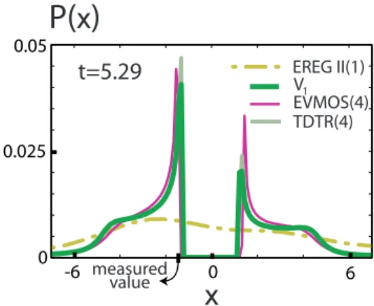
ensemble members into two separate regions is well repro-duced by EVMOS (as well as TDTR), but due to the random noise this feature is no longer present for lead timest >5 in the EREG II forecast. The absence of the bimodality of the EREG II distribution for the variablex at lead timet=5.29 is clearly seen in Fig. 16.
6 Conclusions
Several linear regression methods have been tested in the context of post-processing of (ensemble) forecasts: classi-cal linear regression, total least-square regression, Tikhonov regularization, error-in-variable regression, geometric mean regression and best-member regression. These approaches were evaluated based on three criteria (see Table 1): a cor-rection of the forecast error, the ability to cope with multi-collinearity and the reproduction of the observed variability. The regression schemes have been tested in the context of the low-order Lorenz 1963 system by introducing both model and initial-condition errors. Three timescales may be distin-guished. First, for short lead times, strong error improve-ments and an increase of ensemble spread-error correlations may be obtained in case of large model errors. Except for GM, skill at these timescales does not so much depend on which regression method is applied, but rather on how many and which predictors are selected. Second, at intermediate times, when the error (and all the moments of its distribu-tion) undergoes fast growth, all regression methods, except
0 1 2 3 4 5 6 7
−20 −10 0 10
20
Uncorrected Forecast V
0 1 2 3 4 5 6 7
−20 −10 0 10
20
EREG II (1)
0 1 2 3 4 5 6 7
−20 −10 0 10 20
EVMOS (4)
1t
t
t
x
x
x
Fig. 15.Time evolution of the variablexfor ten ensemble members (full lines) using the Lorenz model generated by the uncorrected forecastV1, EREG II and EVMOS(4). The blue dashed line
indi-cated the evolution of the observation. All ensemble members are initialized using an initial condition spread 10−1around the starting point(x,y,z)=(−11.84,−4.484,38).
0.025 0.05
0
-6 0 6
EVMOS(4) TDTR(4) EREG II(1) V
P(
x
)
1
t=5.29
x
measured value
for EREG II and GM, yield the same result. EREG II and GM provide less favorable results. Third, for long times, when the correlation between the measurement variable and the predictors is almost zero, strong differences between the regression methods are visible. TLS yields a wild and un-physical forecast; the OLS and EREG I corrected forecasts converge towards climatology.
The EREG II method has the benefit to account for the lack of variability which is featured in the EREG I method and, thus, satisfies criterion (iii). Also it provides a mean en-semble spread which is very close to the MSE of the ensem-ble mean, a property often required in an operational con-text. However, all this is done by construction: random noise is addeda posteriori to the EREG I forecast. This implies that some essential statistical information of the underlying physics is lost, such as the specific multiple-peak structure of the error distribution and the non-Gaussian nature of the probability distribution of the variables themselves. A simi-lar behaviour is encountered in an operational context when EVMOS was compared with the non-homogeneous Gaussian regression method, the latter smoothing out the multimodal structure of the forecast (Vannitsem and Hagedorn, 2011). Also, at long lead times EREG II, as well as OLS and EREG I, has a reduced spread-error correlation as compared to the uncorrected and the EVMOS forecast.
Another technique exists in the literature based on the po-tential relation between the different observables effectively measured (Perfect Prog, Klein et al., 1959; Wilks, 2006). This approach does not suffer from the convergence towards climatology like OLS. However, the correction obtained with this technique is useless for sufficiently small forecast error. We have performed a preliminary exploration of this aspect by applying Perfect Prog for the Lorenz system. For each variable X, Y, Z, we have built a Perfect Prog relationship based on the two other variables of our reference system. In this case, Perfect Prog becomes useful when errors reach val-ues of the order of 1/5 of the saturation error variance shown in Fig. 5.
The techniques as presented here can be extended to com-bine multimodel forecasts (e.g. Pe˜na and Van den Dool, 2008). A straightforward way would be to use the different forecasts as predictors. Regression corresponds to a method for “weighting” the different models. However, since many such models may contain the same information, one must be sure that the regression method is able to cope with multi-collinearity. TDTR and EVMOS can fulfil this requirement.
Appendix A
A1 Derivation of EVMOS solution
In this Appendix, we provide additional calculations con-cerning the EVMOS method as introduced in Sect. 3.4. The EVMOS cost functionJEVof Eq. (21) can be rewritten as a
sum over all forecasts:
JEV(β,ξ)= X
n
P
p(Vnp−ξnp)βp
σXC !2
+ Xn−
P pξnpβp
σX
!2 . (A1)
First, we minimize with respect toξnp. This yields: X
p
βpξnp=
σX2PpβpVnp+σX2CXn
σX2+σX2 C
, (A2)
and substitution in Eq. (A1) gives:
JEV(β)= P
n
Xn−PpβpVnp
2
σX2+σX2 C
.
The variance of the predictand σX2
C can be written as
P
p1,p2βp1hVp1Vp2iβp2. Minimization with respect to βt
then gives:
X
p
hVtVpiβp− hVtXi !
σX2+X
p1,p2
βp1hVp1Vp2iβp2 !
= X
p
hVtVpiβp !
σX2+X
p1,p2
βp1hVp1Vp2iβp2
−2X
p
hXVpiβp !
. (A3)
We introduce now the vector β with components βp=
βpcXp wherecXp= hXVpi, and the matrix ρ with
compo-nentsρp1p2= hVp1Vp2i/(cXp1cXp2). After some calculation,
Eq. (A3) reduces to:
βTρβ−21T·ββTρ= −σX21, (A4)
with1a vector with all itsP components equal to one. One can check that the following solution satisfies Eq. (A4):
β= σX ρ
−1·1
p
1T·ρ−1·1, (A5)
which is identical to the solution given in Eq. (24). Note that the expression under the square-root sign is always positive sinceρis a correlation matrix and is, therefore, positive def-inite, as well as its inverse.
Appendix B
B1 Numerical method for nonlinear GM regression The GM cost function Eq. (29) can be minimized using the iterative Gauss-Newton methods for least-square problems (see for example Bj¨orck, 1996). First of all, the cost function can be written as a function of the matrixr:
wherer(β)=(X−Vβ)/N andN(β)= Qpβp
1/2P. Then given at stepkthe valuesrk and the regression coefficients
βk, the coefficients at stepk+1 by assuming small changes are searched1β=βk+1−βk. Therefore,rn(β)at stepk+1
becomes: r
βk+1
≈r
βk
+Jk1β, (B2)
where the matrixJnp=∂rn/∂βp, evaluated at stepk.
Substi-tuting Eq. (B2) into the cost function Eq. (B1) at time step k+1 and expanding to second order yields:
JGMk+1(β)≈rT·r+1βTJTJ1β+2rTJ1β, (B3) where again, all is evaluated at time stepk. Minimization with respect to1βgives:
1β= −(JTJ)−1JTr. (B4) So far, the derivation was general. Substituting now the cost function of the GM approach, one gets:
1βp=βp(A−1B)p, (B5)
where:
Ap1p2=Cbp1p2+
β−bC·1
p1
+β−bC·1
p2
2P
+σ
2 X+1
T·bC·1−2(1T·β)
(2P )2 ,
B=β−bC·1
2P +
σX2+1T·Cb·1−2(1T·β) (2P )2 ,
where we introduced the notations bCp1p2 =ρp1p2βp1βp2,
βp=βpcXpand1is a vector containingP times the scalar
one. We may now calculateβk+1=1β+βk and continue this procedure to time stepk+1 until convergence is reached.
Acknowledgements. We thank Anastasios Tsonis and an
anony-mous reviewer for their constructive comments. This work is supported by the Belgian Science Policy Office under contract MO/34/020.
Edited by: J. Duan
Reviewed by: A. Tsonis and another anonymous referee
References
Bj¨orck, A.: Numerical methods for least-square problems, SIAM, Philadelphia, 408 pp., 1996.
Casella, G. and Berger, R. L.: Statistical Inference, Brooks Cole Publishing, 661 pp., 1989.
Draper, N. R. and Yang, Y.: Generalization of the geometric-mean functional relationship, Comput. Stat. Data An., 23, 355–372, doi:10.1016/S0167-9473(96)00037-0, 1997.
Glahn, B., Peroutka, M., Wiedenfeld, J., Wagner, J., Zylstra, G., Schuknecht, B., and Jackson, B.: MOS Uncertainty Estimates in an Ensemble Framework, Mon. Weather Rev., 137, 246–268, 2009.
Golub, G. H. and Van Loan, C. F.: Matrix computations, 794 pp., 1996.
Grimit, E. P. and Mass, C. F.: Measuring the ensemble spread-error relationship with a probabilistic approach: stochastic ensemble results, Mon. Weather Rev., 135, 203–221, 2007.
Iversen, T., Deckmyn, A., Santos, C., Sattler, K., Bremnes, J. B., Feddersen, H., and Frogner, I.-L.: Evaluation of “GLAMEPS” – a proposed multi-model EPS for short range forecasting, Tellus A, in press, doi:10.1111/j.1600-0870.2010.00507.x, 2010. Klein, W. H., Lewis, B. M., and Enger, I.: Objective prediction of
five-day mean temperatures during winter, J. Meteor., 16, 672– 682, 1959.
Leutbecher, M. and Palmer, T. N.: Ensemble forecasting, J. Com-put. Phys., 227, 3515–3539, 2008.
Lorenz, E. N.: Deterministic non-periodic flows, J. Atmos. Sci., 20, 130–141, 1963.
Pe˜na, M. and Van den Dool, H.: Consolidation of Multimodel Fore-casts by Ridge Regression: Application to Pacific Sea Surface Temperature, J. Climate, 21, 6521–6538, 2008.
Teisser, G.: La relation d’allom´etrie sa signification statistique et biologique, Biometrics, 4, 14, 1948.
Unger, D. A., van den Dool, H., O’Lenic, E., and Collins, D.: En-semble Regression, Mon. Weather Rev., 137, 2365–2379, 2009. Van Huffel, S. and Vandewalle, J.: The total least-square
prob-lem: Computational aspects and analysis, SIAM, Philadelphia, 300 pp., 1991.
Van den Dool, H. M.: Empirical Methods in Short-Term Climate Prediction, Oxford University Press, 215 pp., 2006.
Vannitsem, S.: Dynamical Properties of MOS Forecasts: Analysis of the ECMWF Operational Forecasting System, Weather Fore-cast., 23, 1032–1043, 2008.
Vannitsem, S.: A unified linear Model Output Statistics scheme for both deterministic and ensemble forecasts, Q. J. Roy. Meteorol. Soc., 135, 1801–1815, 2009.
Vannitsem, S. and Hagedorn, R.: Ensemble forecast
post-processing over Belgium: Comparison of deterministic-like and ensemble regression methods, Meteorol. Appl., 18, 1, 94–104, March 2011.
Vannitsem, S. and Nicolis, C.: Dynamical Properties of Model Out-put Statistics Forecasts, Mon. Weather Rev., 136, 405–419, 2008. Wilks, D. S.: Statistical methods in the atmospheric sciences,