Northern Hemisphere deglaciation
H. Goelzer1, I. Janssens1, J. Nemec1,*, and P. Huybrechts1
1Earth System Sciences & Departement Geografie, Vrije Universiteit Brussel, Brussels, Belgium *now at: Zentralanstalt f¨ur Meteorologie und Geodynamik, Vienna, Austria
Correspondence to:H. Goelzer ([email protected])
Received: 15 September 2011 – Published in Geosci. Model Dev. Discuss.: 20 October 2011 Revised: 31 March 2012 – Accepted: 16 April 2012 – Published: 9 May 2012
Abstract.We describe and evaluate a dynamical
continen-tal runoff routing model for the Northern Hemisphere that calculates the runoff pathways in response to topographic modifications due to changes in ice thickness and isostatic adjustment. The algorithm is based on the steepest gradient method and takes as simplifying assumption that depressions are filled at all times and water drains through the lowest out-let points. It also considers changes in water storage and lake drainage in post-processing mode that become important in the presence of large ice dammed proglacial lakes. Although applicable to other scenarios as well, the model was con-ceived to study the routing of freshwater fluxes during the last Northern Hemisphere deglaciation. For that specific applica-tion we simulated the Northern Hemisphere ice sheets with an existing 3-D thermomechanical ice sheet model, which calculates changes in topography due to changes in ice cover and isostatic adjustment, as well as the evolution of fresh-water fluxes resulting from surface ablation, iceberg calving and basal melt. The continental runoff model takes this input, calculates the drainage pathways and routes the freshwater fluxes to the surface grid points of an existing ocean model. This results in a chronology of temporally and spatially vary-ing freshwater fluxes from the Last Glacial Maximum to the present day. We analyse the dependence of the runoff routing to grid resolution and parameters of the isostatic adjustment module of the ice sheet model.
1 Introduction
The problem of finding the runoff pathways and drainage basins for a given topographic setting is crucial for questions in a wide range of scientific fields ranging from hydrology to climatology and environmental studies, to name only a few examples. Determining the runoff pathways for a study area is not evident with regard to issues of scale, resolution and water storage. Since the advent of digital elevation models (DEM), computational routines have been proposed that sim-plify the process in many ways and allow for at least semi-automatic procedures to delineate the pathways and drainage basins (e.g. Tarboton, 1991; Renssen and Knoop, 2000; D¨oll and Lehner, 2002). This has made routing runoff over a ter-rain a standard procedure in geographic information system applications.
basins (Masutomi et al., 2009). Apart from the runoff direc-tion, the temporal characteristics of runoff can be captured using network response functions (Gong et al., 2009), which include the effect of local short-term water storage.
All of the described refinements depend on data availabil-ity and to a lesser extent on the possibilavailabil-ity to compare results to present-day observations in the form of stream gauge sta-tions. For paleo-applications, the focus of the present work, such specific data (e.g. on past river locations) are sparse or simply not available, which simplifies the task but also in-troduces uncertainties in the runoff predictions. In addition, details of the temporal characteristics of the routing network are not crucial to resolve. Water travel time through the net-work, typically of the order of days, may safely be ignored given the long response time scales of interest.
The runoff model described in this paper was conceived and tested for one specific paleo-application: the decay of the Northern Hemisphere ice sheets during the last deglaciation and the Holocene (21–0 kyr BP). Aside from the associated large changes in topography and albedo, their freshwater dis-charge probably had strong effects on the ocean circulation and on the global temperature evolution during this period. Paleoclimatic evidence suggests that rapid climate changes during the glacial cycles can be associated with reorganisa-tions of the ocean-atmosphere system (e.g. Broecker et al., 1985; Clark et al., 2002). The location of freshwater enter-ing the ocean is thereby thought to have a strong control on the evolution of the ocean circulation (e.g. Broecker et al., 1990). To study possible changes in the ocean circulation, it is therefore crucial to track both the intensity and location of glacial melt water runoff and of iceberg calving.
While the routing of freshwater for a given topography is a standard procedure, and an example exists for the time period of the last deglaciation (Tarasov and Peltier, 2005), our model is specifically aimed for and ready to be coupled to an ocean model. We therefore address the problems that arise from the combination of a temporally changing topog-raphy (as a function of evolving ice thickness and isostatic adjustment) with an ocean model grid that uses a fixed land-sea mask. This represents an important step towards coupled ice-sheet-ocean model simulations. At present, ocean models that allow for a temporally variable bathymetry and land-sea mask are not readily applied on a global scale and time scales of glacial-interglacial transitions, due to computational limi-tations. In our application, we therefore deal with a constant ocean model grid in combination with a variable land-sea mask of the ice sheet model. The mismatch between ice sheet and ocean model grids has to be taken into account, and the changing topography makes it necessary to regularly update the routing matrix automatically and in a computationally ef-ficient way.
2 Model setup
The continental runoff model (CRM) described in this pa-per is a new module to an existing Northern Hemisphere ice sheet model (NHISM, Zweck and Huybrechts, 2005) and serves as interface to an ocean model (CLIO, Goosse and Fichefet, 1999). Before describing the CRM in detail, we first give a brief overview of the ocean model grid and the ice sheet model. Although developed specifically for the given model setup as interface between NHISM and CLIO, the fundamental formulation of CRM could be applied to other combinations of ice sheet and ocean models and for other applications, where the routing matrix has to be updated au-tomatically.
2.1 The Northern Hemisphere ice sheet model
The ice sheet model used for the present study merely serves to illustrate the use of the continental runoff model, so only a short description is given here. NHISM, a three-dimensional thermomechanical ice dynamic model consist of three main components which respectively describe the ice flow, the solid Earth response and the mass balance at the ice-atmosphere interface (Huybrechts and T’siobbel, 1995; Huybrechts and de Wolde, 1999; Huybrechts, 2002). In many ways the model is similar to other large-scale ice sheet mod-els (e.g. Ritz et al., 1996; Greve, 1997) based on the shallow ice approximation, which drastically simplifies the calcula-tion of ice velocities. NHISM only considers grounded ice and therefore does not account for ice shelf dynamics. Nev-ertheless, marine ice dynamics is included with a parame-terization for marine calving that allows determining the ex-tent of ice grounded below sea level (Zweck and Huybrechts, 2003). Freshwater fluxes from the ice sheet consist of spa-tially resolved surface ablation, calving at the margin and basal melting. The isostatic adjustment module included in NHISM accounts for changes of the Earth surface due to the evolving weight of the ice. It principally consists of two separate layers of the Earth’s mantle, an elastic plate (litho-sphere) and a viscously deforming layer with a character-istic adjustment time scale τ underneath it (astenosphere).
The lithospheric treatment accounts for a flexural rigidityD,
meaning that aside from local isostasy, contributions from re-mote locations are taken into account as well (Le Meur and Huybrechts, 2001). Note that limitations of this type of iso-static model have been reported when applied for glacial cy-cle modelling of Eurasia (van den Berg et al., 2008).
2.2 The ocean model grid
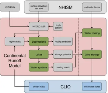
Fig. 1.Overview of the Continental Runoff Model and of exchanges with the ice sheet model (NHISM) and the ocean model (CLIO). The processing chain on the right hand side displays how freshwater fluxes from the ice sheets are routed to appropriate oceanic grid cells.
LOVECLIM (Goosse et al., 2010). In order to avoid singu-larities at the poles of the coordinate system, two spherical subgrids are used in this model, for which the poles are not located in the ocean domain. The first one is based on clas-sical longitude-latitude coordinates. It covers the Southern Ocean, the Pacific Ocean, the Indian Ocean and the South Atlantic. The remaining parts of the ocean (i.e. the North At-lantic and the Arctic) are represented on the second spher-ical subgrid, which has its poles located at the equator, the “North Pole” in the Pacific and the “South Pole” in the In-dian Ocean. The two subgrids of both 3×3◦horizontal
res-olution are connected in the equatorial Atlantic where there is a correspondence between the meridians of the South At-lantic on one grid and the parallel in the North AtAt-lantic on the other grid. In the model, the two subgrids are considered as a single coordinate system using metric coefficients, which are given by Deleersnijder et al. (1993).
2.3 Continental runoff model
For a given surface topography, the continental runoff model (CRM) calculates the runoff pathways and connects each continental point with an oceanic grid point to which freshwater fluxes can be delivered. The basic assumptions are that water does not evaporate nor infiltrate in the underlying layers and that enough water is available to fill up continen-tal depressions. We furthermore ignore temporal aspects of the routing process assuming an instantaneous redirection of freshwater fluxes, which is a good approximation for the time scales under consideration here. Topographic changes are in
Fig. 2.HYDRO1kSP DEM (6.25 km resolution) with superimposed
present-day ice thickness from the embedded NHISM grid (black contours).
this study calculated by NHISM and consist of both changes in ice thickness and isostatic adjustment of the Earth’s crust. An overview of the model components and processing steps is given in Fig. 1 and is described in the following subsec-tions.
2.3.1 Updating the relief map
To properly calculate continental drainage paths it is deci-sive to have a high-resolution topographic map, resolving as many features of the surface terrain as possible. Furthermore, the model domain needs to be sufficiently large to allow wa-ter to flow to the appropriate river mouth, at possibly long distances over the continents before reaching the ocean. Con-sequently, we decided to combine topographic changes as calculated by NHISM (50×50 km resolution) with a
hydro-logically correct present-day digital elevation model (DEM) at 1×1 km resolution, called HYDRO1k (http://gcmd.nasa.
gov/records/GCMD HYDRO1k.html). The dataset does not contain bedrock information of, e.g. the Great Lakes and of ocean bathymetry. It was therefore combined with a 1′
res-olution DEM with global coverage (ETOPO1; Amante and Eakins, 2009).
To combine the HYDRO1k map with topographic changes from NHISM they both need to be transformed into a com-mon grid. Therefore, HYDRO1k was transformed to a Po-lar Stereographic projection with standard parallel at 60◦N
(hereafter called HYDRO1kSP) by means of 2-dimensional Lagrange polynomials. Subsequently, NHISM output was interpolated onto this new grid, which has a resolution of 6.25×6.25 km (Fig. 2). While the NHISM grid is limited
R2 R3 R4 R5 d1
d2
d3 d4
d5
d6
d7 L1
L2
L3
L4
L5
R1
CLIO grid
Sea level
Depth threshold
Fig. 3.Schematic delineation of different topographic regions R1 to
R5. Depressions are marked d1 to d7 and lakes L1 to L5. All grid points connected to the same lowest point of a depression (example d2) form a drainage basin (red). Drainage basins connected to the same lake (example L2) form a lake catchment (green). See text for further details.
grid are linearly phased out to zero at the map boundary of HYDRO1kSP.
2.3.2 Constructing a region mask
Since CRM is constructed as interface between NHISM and CLIO, continental drainage areas have to be grouped and connected to grid boxes of that specific ocean model. While the drainage is calculated for a temporally changing land-sea mask on the HYDRO1kSP grid, the runoff has to be mapped to the much coarser and fixed CLIO grid. Conse-quently, coastal points on the HYDRO1kSP grid may not be-long to any of the oceanic CLIO grid boxes. Another prob-lem arises from inland grid points below sea level, e.g. in the Caspian Sea, which have to be connected to the CLIO grid as well. We therefore follow the approach of Tarasov and Peltier (2005) to introduce a depth threshold and search the routing end point of any continental grid point 600 m or deeper below current sea level. Furthermore, we increase the ocean mask by extending it radially around each CLIO grid point. To connect routing end points that are still outside the extended ocean mask, e.g. in the Black Sea and Red Sea, a search algorithm is used, which locates the closest CLIO grid point. A similar complication arises from the limits of the HYDRO1kSP domain. Continental regions that are inter-sected by the model domain boundary also have to be con-nected to the closest ocean grid point using the same search routine. Given all the complications, a combined mask of the following regions is constructed on the HYDRO1kSP grid (Fig. 3):
1. Continental border region: combines all grid points above sea level at the edge of the HYDRO1kSP domain. 2. Continental region: combines all grid points above sea
level except for R1.
a
b
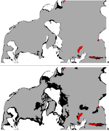
Fig. 4.Ocean mask and topographic regions for the LGM(a)and
the present day(b). Regions with a depth between current sea level and the depth threshold (R3, black) close the gap between topo-graphic coast (R2, grey) and extended ocean mask (R5, white). Map border points (R1, unmarked) and internal ocean regions, which are below the depth threshold but not part of the extended ocean mask (R4, red) are mapped to nearby ocean grid points.
3. Shallow water region: combines all grid points between sea level and the specified depth threshold.
4. Internal ocean region: combines grid points below the depth threshold outside the CLIO ocean mask.
1
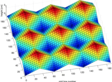
Fig. 5.Ripple pattern overlaid on the raw topography relief map to
decrease computational costs in the solver in flat areas. The ripple depth of several centimetres is negligible compared to real topo-graphic surface features.
2.3.3 Calculation of depressions, lakes and water
systems
Given the surface relief map and a sea level dependent region mask, the inventory of the continental runoff pathways can be pursued. As a pre-processing step, a ripple pattern is su-perimposed on the relief map (Fig. 5), in order to reduce the processing time, which arises from assembling a large num-ber of small depressions into units of larger scale. The depth of these ripples of several centimetres can be neglected com-pared to the size of real topographic surface features. A sub-stantial gain of model run time is achieved mainly when pro-cessing flat surface features, while the global drainage pat-tern remains the same compared to using the unprocessed relief map.
For each grid point, the surface gradient is followed to the lowest grid point in a depression that can be reached. If the lowest point is a deep ocean, internal ocean or border point, it qualifies as an end point to the total routing. All grid points that share the same lowest point are identified and form one of a large number of indexed “drainage basins”. Individual drainage basins are grouped into “lake catchments”, which comprise all drainage basins that are connected to the same lake when the relief is completely filled with water. At this point the outlet of each lake is determined, and the lake vol-ume is computed for later use in the lake storage module. In turn, the lake catchments are grouped into “water systems” consisting of a cascade of lakes that have connected outlets. Water from the lowest lake in a water system can be drained to a specific ocean grid point, since the outlet of the lowest lake is by definition connected to an end point in the deep ocean, internal ocean or on the map boundary. All water sys-tems with endpoints belonging to the same CLIO grid are
Fig. 6.Drainage basins for the present-day topography derived with
CRM(a), where each colour represents a region that drains into the same ocean grid box (shown in grey over the ocean).(b)Level one drainage delineation from the HYDRO1k data set.
taken together (Fig. 6a). Since NHISM calculates freshwa-ter fluxes on a 50×50 km grid resolution, the centre of the NHISM grid box is used to define the entry point into the higher resolution HYDRO1kSP routing grid.
2.3.4 Lake storage module
the model itself, but rather has to be chosen by the user. A guideline for this model parameter choice may be found in paleo-evidence of past large scale drainage events and fur-thermore has to be in line with the sensitivity of the ocean model and its capability to deal with large amounts of lo-calized freshwater input (e.g. Manabe and Stouffer, 1997; Renssen et al., 2001).
3 Results
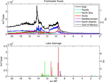
The first immediately available result of CRM is the delin-eation of drainage regions that are connected to the same ocean grid box (Fig. 6a), and which will be discussed in more detail in the next section. Changes of the surface to-pography over time due to changes in ice cover, sea level and isostatic adjustment lead to a reorganisation of the drainage regions. While these are interesting in their own rights, it is both more instructive and physically meaningful to group the different drainage regions into larger units, according to the ocean domains the runoff is directed to. Freshwater fluxes from the ice sheets during the last deglaciation are thought to have had a strong impact on the oceanic circu-lation (Broecker et al., 1985), while their location of impact is discussed as an important factor (e.g. Tarasov and Peltier, 2005). The division of drainage domains here is for diag-nostic purposes only and somewhat arbitrary, but motivated by these research questions. The same grouping of drainage basins has been used to display the time series of runoff par-tition and lake drainage events from the decaying Northern Hemisphere ice sheets over the history of the last deglacia-tion and the Holocene (Fig. 7), which we give here for il-lustrative purposes only. It is beyond the scope of this paper, with focus on the CRM model description, to compare the location and timing against results of other models or geo-logical reconstructions.
Lake drainage events (Fig. 7, bottom) that can exceed the volume flux from direct freshwater runoff arise in relation to major reorganisations of the routing matrix and when ice dammed lakes suddenly drain due to removal of the ice bar-rier.
3.1 Model validation for the present-day topography
For the present-day configuration the derived drainage net-work can be compared to major observed river netnet-works, even if some ocean grid points in the model receive input from more than one river system. We have compared the re-sults on a visual basis with maps from the “Watersheds of the World” study of the World Resource Institute (Revenga et al., 1988) and from “The Times Atlas of the World” (Times Books, 1998). To validate the performance of the model further, we have compared the results with the level one drainage basins of the HYDRO1k data set (Fig. 6). The de-lineation of drainage basins in CRM is overall in good
agree-Fig. 7.Freshwater contributions to different ocean basins (top) and
lake drainage events (bottom) for a transient deglaciation experi-ment.
ment with the data. At this stage it is difficult to separate the influence of the ice sheet and isostatic models, which adds uncertainty to simulations and makes it difficult to evaluate the model during past periods. There is however a growing body of geomorphological data that can eventually be used to constrain the model (e.g. Toucanne et al., 2010).
3.2 Model sensitivity to grid resolution
low resolution DEMs. Without modifications, the size of the Mississippi drainage basin would equally be too small in our coarse resolution models, due to the unresolved nar-row valley of the Missouri river in North Dakota. Its runoff would be blocked and water would be redirected to the north instead of to the south. These differences to the observed delineations have been resolved by minor local editing of the DEM to achieve a more accurate present day basin di-vide. The changes made for the present-day configuration is promising to also hold for past configurations, given that ice thickness evolution and isostatic adjustment in our model change the terrain on a relatively larger spatial scale com-pared to the small compromising topographic features. How-ever, Tarasov and Peltier (2006) report on the necessity to take into account changes in past sill elevations for an accu-rate deglacial drainage calculation on 50 km resolution.
For the comparison between different horizontal resolu-tions of the DEM, we exclude lake storage effects in the model, which guarantees that the total amount of runoff is identical in all four experiments at any time. This also makes it possible to trace the origin and destination of individual changes in the runoff time series.
The routing pattern on a local scale, i.e. on the level of individual water systems and of regions connected to in-dividual ocean grid boxes, shows some variations between different horizontal resolutions of the DEM (not shown). In contrast, the amplitude of drainage to the large-scale ocean basins is largely similar between different resolutions (Fig. 8), except for the lowest resolution of 50 km. The small differences in freshwater flux between the other experiments (resolution 6.25 km, 12.5 km and 25 km) can be expected to have a minor influence on the large-scale ocean and climate model response in a coupled model setup. The above compar-ison therefore shows that a DEM resolution of 25 km is suf-ficient for our aim to model the freshwater routing for such an application. It would be difficult to justify a manifold in-crease in computing time using a higher resolution version of the DEM.
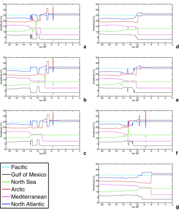
3.3 Model sensitivity to changes of the isostatic adjustment module
In order to study the sensitivity of CRM to changes in iso-static adjustment, we use the same parameter modifications
over its full possible range of values, from instantaneous iso-static adjustment (τ =0 ka, LT0k) to adjustment time scales
of 1000, 3000 and 10 000 yr (LT1k, REF, LT10k) and no ad-justment at all (τ infinite, LTinf).
Similar to the procedure for resolution experiments we ig-nore lake storage contributions for this comparison of differ-ent isostatic model parameters, and, building on the findings above, we use a lower model resolution (25 km) in order to save computing time. Since the ice sheet evolution now dif-fers between experiments, which complicates the compari-son we prescribe a spatially constant freshwater input over the whole model domain. This is crucial for the interpreta-tion of changes in the routing direcinterpreta-tion independent from the effect of varying local freshwater availability (Fig. 9).
The case of no adjustment (LTinf, Fig. 9g) shows changes in the routing direction as a function of ice thickness changes only. Note however that the resulting Northern Hemisphere ice sheets in this case are higher and larger compared to the reference case. The suppressed downward response of the bedrock makes the ice sheets grow higher by strength-ening the elevation-temperature feedback. Transitions to the final interglacial configuration consequently appear later in LTinf compared to the case of instantaneous adjust-ment (LT0k, Fig. 9d) and tentatively, subsequently earlier in LT10k (Fig. 9f), the reference case (REF, Fig. 9a) and LT1k (Fig. 9e). Changes in lithospheric rigidityD(compare
Fig. 9a, b and c) have less importance for the routing than changes in the astenosphere adjustment time scale τ. The
overall picture that emerges is that changes in the isostatic adjustment module have a large influence on the resulting routing time series. This could have been expected due to the large range of parameter modifications especially for the adjustment time scaleτ. The present-day routing partition
between the oceanic basins is however very similar between the different cases, because the DEM is relaxed towards the present-day configuration.
a
b
c
0 0.1 0.2 0.3 0.4
Sv
20 18 16 14 12 10 8 6 4 2 0
0 2000 4000 6000 8000 10000 12000 14000
km
3/year
kyr BP
Pacific Gulf of Mexico North Sea Arctic Mediterranean North Atlantic
b
Fig. 8.Sensitivity of runoff partition between major oceanic basins to changes in DEM resolution.(a)50 km, (b)25 km, (c)12.5 km,
(d)6.25 km.
Table 1.Parameter settings for isostatic sensitivity experiments.
Name REF LR0.1 LR0 LT0k LT1k LT10k LTinf
Lithospheric rigidityD(Nm) 1025 1024 0 (loc.) 1025 1025 1025 1025
Astenosphere adjustment time scaleτ(yr) 3000 3000 3000 0 (inst.) 1000 10000 Inf (none)
Panel in Fig. 9 a b c d e f g
time series down to 50 km resolution of the DEM for the se-lected parameters.
4 Conclusion and discussion
A continental runoff routing model has been presented, which dynamically updates the freshwater routing matrix in response to topographic changes and takes lake storage ef-fects into account in offline mode. The model output was compared against present-day observed river networks and applied for illustrative purposes in the framework of simu-lating the last deglaciation of the Northern Hemisphere ice sheets.
It was shown that the large-scale ocean basins and timing of major freshwater forcing periods is relatively stable be-tween versions of different DEM resolution. For the range of DEM resolutions under scrutiny, the lowest resolution suf-ficient for calculating the large-scale runoff pathways neces-sary to determine the routing of freshwater fluxes to an ocean model is 25 km. Changes in the isostatic adjustment module of the ice sheet model have a strong impact on the timing and direction of runoff routing. This is especially true for modi-fications of the lithosphere adjustment time scaleτ.
b
e
c
f
g
Fig. 9.Sensitivity of runoff partition between major oceanic basins to changes in the isostatic module of the ice sheet model.(a)Reference
run [REF], changes of the lithospheric rigidity LR0.1(b), LR0(c)and changes of adjustment time scale LT0k(d), LT1k(e), LT10k(f), LTinf(g). Parameter values are given in Table 1. The freshwater input was set spatially constant over the entire model domain in order to remove the effect of local freshwater availability. See text for details.
matrix could in principle be used in a fully coupled sys-tem to also route the runoff from precipitation over ice-free land. This would add another source of spatial and tempo-ral variability to the freshwater forcing of the ocean and has the potential to increase the importance of routing direction changes.
As a further development for coupled ice sheet-CRM ex-periments, changes in water loading could be submitted to
Acknowledgements. We acknowledge support through the Belgian Federal Public Planning Service Science Policy Research Pro-gramme on Science for a Sustainable Development under Contracts SD/CS/01A (ASTER) and SD/CS/06A (iCLIPS).
Edited by: R. Marsh
References
Amante, C. and Eakins, B. W.: ETOPO1 1 Arc-Minute Global Relief Model: Procedures, Data Sources and Analysis, NOAA Technical Memorandum NESDIS NGDC-24, 2009.
Broecker, W. S., Peteet, D. M., and Rind, D.: Does the ocean-atmosphere system have more than one stable mode of operation, Nature, 315, 21–26, doi:10.1038/315021a0, 1985.
Broecker, W., Peng, T., Jouzel, J., and Russell, G.: The magnitude of global fresh-water transports of importance to ocean circulation, Clim. Dynam., 4, 73–79, doi:10.1007/BF00208902, 1990. Clark, P. U., Pisias, N. G., Stocker, T. F., and Weaver, A. J.: The
role of thermohaline circulation in abrupt climate change, Na-ture, 415, 863–869, doi:10.1038/415863a, 2002.
Coe, M.: Modeling terrestrial hydrological systems at the continental scale: Testing the accuracy of an atmo-spheric GCM, J. Climate, 13, 686–704, doi:10.1175/1520-0442(2000)013<0686:MTHSAT>2.0.CO;2, 2000.
Deleersnijder, E., Van Ypersele, J.-P., and Campin, J.-M.: An orthogonal curvilinear coordinate system for a world ocean model, Ocean Model., (newsletter), 100, 7–10, (unpublished manuscript), 1993.
D¨oll, P. and Lehner, B.: Validation of a new global 30-min drainage direction map, J. Hydrol., 258, 214–231, doi:10.1016/S0022-1694(01)00565-0, 2002.
Gong, L., Wid´en-Nilsson, E., Halldin, S., and Xu, C.-Y.: Large-scale runoff routing with an aggregated network-response function, J. Hydrol., 368, 237–250, doi:10.1016/j.jhydrol.2009.02.007, 2009.
Goosse, H. and Fichefet, T.: Importance of ice-ocean interactions for the global ocean circulation: A model study, J. Geophys. Res., 104, 23337–23355, doi:10.1029/1999JC900215, 1999.
Goosse, H., Brovkin, V., Fichefet, T., Haarsma, R., Huybrechts, P., Jongma, J., Mouchet, A., Selten, F., Barriat, P.-Y., Campin, J.-M., Deleersnijder, E., Driesschaert, E., Goelzer, H., Janssens, I., Loutre, M.-F., Morales Maqueda, M. A., Opsteegh, T., Mathieu, P.-P., Munhoven, G., Pettersson, E. J., Renssen, H., Roche, D. M., Schaeffer, M., Tartinville, B., Timmermann, A., and Weber, S. L.: Description of the Earth system model of intermediate complex-ity LOVECLIM version 1.2, Geosci. Model Dev., 3, 603–633, doi:10.5194/gmd-3-603-2010, 2010.
Greve, R.: Application of a polythermal three-dimensional ice sheet model to the Greenland ice sheet: Response to steady-state and transient climate scenarios, J. Climate, 10, 901–918, doi:10.1175/1520-0442(1997)010<0901:AOAPTD>2.0.CO;2, 1997.
Huybrechts, P.: Sea-level changes at the LGM from ice-dynamic reconstructions of the Greenland and Antarctic ice sheets dur-ing the glacial cycles, Quaternary Sci. Rev., 21, 203–231, doi:10.1016/S0277-3791(01)00082-8, 2002.
Huybrechts, P. and de Wolde, J.: The dynamic response of the Greenland and Antarctic ice sheets to multiple-century cli-matic warming, J. Climate, 12, 2169–2188, doi:10.1175/1520-0442(1999)012<2169:TDROTG>2.0.CO;2, 1999.
Huybrechts, P. and T’siobbel, S.: Thermomechanical modelling of northern hemisphere ice sheets with a two-level mass-balance pa-rameterisation, Ann. Glaciol., 21, 111–116, 1995.
Le Meur, E. and Huybrechts, P.: A model computation of surface gravity and geoidal signal induced by the evolving Greenland ice sheet, Geophys. J. Int., 145, 835–849, doi:10.1046/j.1365-246x.2001.01442.x, 2001.
Manabe, S. and Stouffer, R. J.: Coupled ocean-atmosphere model response to freshwater input: Comparison to Younger Dryas event, Paleoceanography, 12, 321–336. doi:10.1029/96PA03932, 1997.
Maidment, D. R.: GIS and hydrological modeling: an assessment of progress, Paper presented at the Third International Conference on GIS and Environmental Modeling, Santa Fe, New Mexico, 1996.
Masutomi, Y., Inui, Y., Takahashi, K., and Matsuoka, Y.: Develop-ment of highly accurate global polygonal drainage basin data, Hydrol. Process., 23, 572–584, doi:10.1002/hyp.7186, 2009. Renssen, H. and Knoop, J.: A global river routing network
for use in hydrological modeling, J. Hydrol., 230, 230–243, doi:10.1016/S0022-1694(00)00178-5, 2000.
Renssen, H., Goosse, H., Fichefet, T., and Campin, J.: The 8.2 kyr BP event simulated by a global atmosphere-sea-ice-ocean model, Geophys. Res. Lett., 28, 1567–1570, doi:10.1029/2000GL012602, 2001.
Revenga, C., Murray, S., Abramovitz, J., and Hammond, A.: Water-sheds of the World: Ecological Value and Vulnerability, Wash-ington, DC, World Resources Institute, 1998.
Ritz, C., Fabre, A., and Letreguilly, A.: Sensitivity of a Green-land ice sheet model to ice flow and ablation parameters: Con-sequences for the evolution through the last climatic cycle, Clim. Dynam., 13, 11–23, doi:10.1007/s003820050149, 1996. Tarasov, L. and Peltier, W. R.: Arctic freshwater forcing of
the Younger Dryas cold reversal, Nature, 435, 662–665, doi:10.1038/nature03617, 2005.
Tarasov, L. and Peltier, W. R.: A calibrated deglacial drainage chronology for the North American continent: evidence of an Arctic trigger for the Younger Dryas, Quaternary Sci. Rev., 25, 659–688, doi:10.1016/j.quascirev.2005.12.006, 2006.
Tarboton, D. G., Bras, R. L., and Rodrigueziturbe, I.: On the ex-traction of channel networks from digital elevation data, Hydrol. Process., 5, 81–100, doi:10.1002/hyp.3360050107, 1991. Times Books: The Times Atlas of the World, Times Books Limited,
7th Edn., 228 pp. and 123 plates, 1988.
Toucanne, S., Zaragosi, S., Bourillet, J. F., Marieu, M., Cremer, M., Kageyama, M., Van Vliet-Lan¨oe, B., Eynaud, F., Turon, J. L., and Gibbard, P. L.: The first estimation of Fleuve Manche palaeoriver discharge during the last deglaciation: Evidence for Fennoscandian ice sheet meltwater flow in the English Chan-nel ca 20–18 ka ago, Earth Planet. Sci. Lett., 290, 459–473, doi:10.1016/j.epsl.2009.12.050, 2010.