www.hydrol-earth-syst-sci.net/19/1887/2015/ doi:10.5194/hess-19-1887-2015
© Author(s) 2015. CC Attribution 3.0 License.
Spatial sensitivity analysis of snow cover data in a distributed
rainfall-runoff model
T. Berezowski1,2, J. Nossent2, J. Chorma ´nski1, and O. Batelaan2,3
1Department of Hydraulic Engineering, Warsaw University of Life Sciences, Nowoursynowska 166, 02-787 Warsaw, Poland 2Department of Hydrology and Hydraulic Engineering, Vrije Universiteit Brussel, Pleinlaan 2, 1050 Brussels, Belgium 3School of the Environment, Flinders University, GP.O. Box 2100, Adelaide SA 5001, Australia
Correspondence to:T. Berezowski ([email protected])
Received: 17 September 2014 – Published in Hydrol. Earth Syst. Sci. Discuss.: 30 October 2014 Revised: 7 March 2015 – Accepted: 5 April 2015 – Published: 21 April 2015
Abstract.As the availability of spatially distributed data sets for distributed rainfall-runoff modelling is strongly increas-ing, more attention should be paid to the influence of the quality of the data on the calibration. While a lot of progress has been made on using distributed data in simulations of hy-drological models, sensitivity of spatial data with respect to model results is not well understood. In this paper we develop a spatial sensitivity analysis method for spatial input data (snow cover fraction – SCF) for a distributed rainfall-runoff model to investigate when the model is differently subjected to SCF uncertainty in different zones of the model. The anal-ysis was focussed on the relation between the SCF sensitivity and the physical and spatial parameters and processes of a distributed rainfall-runoff model. The methodology is tested for the Biebrza River catchment, Poland, for which a dis-tributed WetSpa model is set up to simulate 2 years of daily runoff. The sensitivity analysis uses the Latin-Hypercube One-factor-At-a-Time (LH-OAT) algorithm, which employs different response functions for each spatial parameter rep-resenting a 4×4 km snow zone. The results show that the
spatial patterns of sensitivity can be easily interpreted by co-occurrence of different environmental factors such as geo-morphology, soil texture, land use, precipitation and temper-ature. Moreover, the spatial pattern of sensitivity under dif-ferent response functions is related to difdif-ferent spatial param-eters and physical processes. The results clearly show that the LH-OAT algorithm is suitable for our spatial sensitivity anal-ysis approach and that the SCF is spatially sensitive in the WetSpa model. The developed method can be easily applied to other models and other spatial data.
1 Introduction
Several studies address classical sensitivity and uncer-tainty analysis methods to spatial data and parameters. An interesting stochastic uncertainty approach for spatial rain-fall fields in the dynamic TOPMODEL (Beven and Freer, 2001) was presented by Younger et al. (2009). The results were obtained by dividing a catchment into homogeneous ir-regular zones in which the precipitation was randomly per-turbed by large factors. Their study, however, focusses on the model output uncertainty rather than on quantification of spatial sources of uncertainty or spatial sensitivity.
Another study is presented by Stisen et al. (2011), who investigated whether the use of spatially distributed surface temperature data in an objective function can provide robust calibration and evaluation of the MIKE SHE model com-pared to a lumped simulation. The study used a spatial per-turbation of parameters by random factors between 0.75 and 1.25 in a 2 km grid for the sensitivity analysis, but the results were not analyzed spatially. Thus no spatial pattern of sensi-tivity, showing which zones of the model are more vulnerable to uncertainty, was obtained.
Another spatial approach for sensitivity analysis was pre-sented by Hostache et al. (2010). In their work a local, gra-dient method was applied to conduct a sensitivity analysis of the Manning coefficient in each computational node of a hy-drodynamic model. This approach showed completely differ-ent sensitivity zonation than in the predefined land-use-based Manning coefficient classes used as a comparison scenario. This result stresses the importance of assessing the sensitiv-ity in a spatially distributed way.
In this study, the various approaches of spatial sensitiv-ity (or uncertainty) analysis presented above are compiled and extended in order to propose a method that would be generally applicable and thus would give a framework for inter-comparison of different models. Such a method would use a regular grid to quantify the spatial pattern of sensitivity as in Stisen et al. (2011); hence it differs from the irregular zonation in Younger et al. (2009). Furthermore, the pertur-bation of spatial input data in a general framework should be realized using a well-established algorithm, e.g. Latin-Hypercube One-factor-At-a-Time (LH-OAT) (van Griensven et al., 2006). This change would give a straightforward inter-pretation of the sensitivity. Similarly, Hostache et al. (2010) used a well-established gradient method for spatial sensitiv-ity analysis. However, unlike the gradient method, LH-OAT provides global insight into sensitivity. Such a method would also allow one to quantify the sensitivity of spatial data with respect to the output and be able to explain the causes for the sensitivity patterns.
The main purpose of the application of spatial sensitivity analysis proposed in this study would be, after the Saltelli (2002) definition of sensitivity analysis, to quantify spatially the vulnerability of the model output to uncertainty of spatial input. Thus a result of this analysis would provide feedback, e.g. in regards to where in a model domain a modeler should focus more on the quality of input data and parameters.
How-ever, the same method can be used for comprehensive spatial change (e.g. land-use change) analyses to show where the change (e.g. urbanization) would be least or most influenc-ing the model output.
An important issue in this study is the selection of the hy-drological model used to conduct the spatial sensitivity anal-ysis. An option is the Water and Energy Transfer between Soil, Plants and Atmosphere (WetSpa) model (De Smedt et al., 2000; Liu and De Smedt, 2004) which has shown to have a high sensitivity with respect to runoff prediction when various scenarios of distributed impervious surfaces input data were tested (Chorma´nski et al., 2008; Berezowski et al., 2012; Verbeiren et al., 2013). Moreover, the WetSpa model allows parametrization based on distributed snow data from a remote sensor (Berezowski et al., 2015).
Another issue is the selection of the input data used to con-duct the spatial sensitivity analysis. A spatial data set that is frequently tested and easy to obtain is snow cover. Snow cover fraction (SCF [-]) or snow water equivalent remote sensing products are widely available from a number of sen-sors. The different available products vary widely in spatial resolution (500 m to 25 km), temporal resolution (sub-daily to monthly) and temporal coverage (the oldest time series starts in 1966, while new products are regularly announced). One of the most frequently used remote sensing snow prod-ucts comes from the MODIS instrument (Hall et al., 2006). Several studies show different strategies with respect to how hydrological models can benefit from MODIS snow cover data. A popular approach is to derive snow depletion curves from MODIS SCF and use them in the Snowmelt Runoff Model (SRM) (Martinec, 1975). This approach is still popu-lar and used in recent studies (Lee et al., 2005; Tekeli et al., 2005; Li and Williams, 2008; Butt and Bilal, 2011; Tahir et al., 2011; Bavera et al., 2012). However, the SRM studies are focussed mostly on the winter half-year and are limited to study sites where snowmelt processes are dominant. Another popular model which benefits from satellite-derived SCF is HBV (Sælthun, 1996), with a number of studies showing use of MODIS snow products (Udnaes et al., 2007; Parajka and Blöschl, 2008; ¸Sorman et al., 2009). In the WetSpa model the MODIS snow products were used to evaluate spatial distri-bution of predicted snow cover (Zeinivand and De Smedt, 2010) and for analysing its skill for discharge simulation (Berezowski et al., 2015). The spatial sensitivity of model output to snow cover, despite its popularity as input data in distributed hydrological models, has not yet been evaluated.
section “Methods” presents the spatially distributed rainfall-runoff model WetSpa, the study area, data and spatial sitivity analysis. In “Results” the output of the spatial sen-sitivity analysis of SCF for the Biebrza River catchment is presented and described. The “Discussion” section presents the results in light of the hydrological processes occurring in the study area, but further applicability of the spatial sensi-tivity analysis method and the limitation of the method (e.g. computation time) are also provided. The final section “Con-clusions” recaps the main findings of the study.
2 Methods
2.1 Hydrological model
The hydrological simulations in this study were conducted using the WetSpa model (De Smedt et al., 2000; Liu et al., 2003). The model divides a catchment into a regular grid with a specified dimension. In each grid cell, the water bal-ance is simulated and the surface, interflow and groundwa-ter discharge components are routed to the catchment outlet (Wang et al., 1996). Spatial parameters used to calculate the hydrological processes are obtained from land-use, soil and elevation input maps. Attribute tables based on literature data are linked to the maps and transformed to distributed phys-ical values via a GIS preprocessing step (Chorma´nski and Michałowski, 2011). Several studies have demonstrated that WetSpa and its steady-state version WetSpass (Batelaan and De Smedt, 2007) are suited to integrate distributed remote sensing input data in the simulation of the hydrological pro-cesses (Poelmans et al., 2010; Dujardin et al., 2011; Ampe et al., 2012; Chorma´nski, 2012; Demarchi et al., 2012; Dams et al., 2013).
The model consists of the following storages: intercep-tion, depression, root zone, interflow and groundwater. Water transport between the storages is based on physical and em-pirical equations. Rainfall, temperature and potential evapo-transpiration based on data from meteorological stations are made spatially explicit by use of Thiessen polygons, but a spatially distributed input form is also possible.
In the standard WetSpa version, snow accumulation is calculated based on precipitation and a threshold temper-ature t0 (◦C). When the temperature in a grid cell is t (◦C) and falls below t0, precipitation is assumed to be snow. Snowmelt is calculated based on t0, a degree-day coefficient ksnow(mm◦C−1day−1) and coefficientkrain (mm mm−1◦C−1day−1), reflecting the amount of snowmelt caused by rainfallvrain(mm). In this study SCF was obtained from MODIS snow products and used as input data. Thus, snow accumulation was not calculated but replaced with the input SCF, while the snowmelt amount (vsm) (mm) per model time stepδt(day) is calculated as
vsm=SCF(ksnow(t−t0)+krainvrain(t−t0)) δt. (1)
This approach of calculating snowmelt based on SCF and snowmelt rate was proposed by Liston (1999). It allows us to obtain distributedvsmvalues weighted by SCF from grid cells where SCF>0. WetSpa is also capable of using an en-ergy balance model for snowmelt calculation (Zeinivand and De Smedt, 2010); however, because of the higher demand on input data, this approach was not used.
Surface water routing is based on a geomorphological in-stantaneous unit hydrograph (IUH) (Liu et al., 2003). The IUH is calculated for a flow path starting in a grid cell and ending at the catchment outlet, i.e. each grid cell has its own IUH. Groundwater flow and interflow are calculated on a sub-catchment level based on a linear reservoir method and routed to the catchment outlet with the IUH. Comparison of the WetSpa performance with other distributed hydrological models can be found in the results of the DMIP2 project (Sa-fari et al., 2012).
The model was set up with a daily time step and 250 by 250 m grid cells. The calibration period was 1 Septem-ber 2008 to 31 August 2009, while validation was from 1 September 2007 to 31 August 2008. The length of the cal-ibration and validation was selected to optimize the model for snow conditions occurring in the period selected for sen-sitivity analysis (Sect. 2.4.1). The global WetSpa parameters were calibrated using the Shuffled Complex Evolution algo-rithm (Duan et al., 1993). The calibration was conducted with the R software (R Development Core Team, 2013) and pack-age “hydromad”. The model was optimized to maximize the Nash and Sutcliffe (1970) efficiency (NSE):
NSE=1−
τ
P
x=1
Qx− ˆQx
2
τ
P
x=1
Qx−Q
2 , (2)
whereQx andQˆxare observed and simulated discharges at
timex,Qis the mean observed discharge andτ is the total number of time steps. Sensitivity of the WetSpa model to the global parameters is presented in Yang et al. (2012).
2.2 Study area
trib-#
! (
! (
! (
! ( !
(
! (
! ( !
(
! (
! ( !
(
! ( !
(
! ( ! ( !
(
! (
! ( !
(
! ( !
(
!
( !(
! (
! (
"
) ")
" )
" ) "
)
Ełk
Netta
Biebrz a
Je grz
nia
Si
dr
a
Br
zo
zó
w
ka
Wissa
Burzyn
0 15 30Km
—
P o l a n d
Legend:
"
) Temperature and precipitation
!
( Precipitation
#
Burzyn profileMain rivers Elevation [m asl]
298
200
102
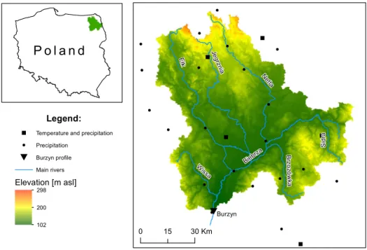
Figure 1.Topography of the study area and location of meteorological stations.
Figure 2.Slope map of the study area.
utaries after the accumulation period. Lakes in WetSpa are modelled by setting appropriate values of the hydraulic pa-rameters in the model, e.g. by a high runoff coefficient and low friction. The simulation of water management schemes in the controlled lakes is, however, not implemented. Dom-inant soil textures in the study area are sand (34 %), loamy sand (26 %) and sandy loam (18 %), whereas minor parts are
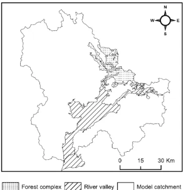
covered by sandy clay (4 %) and silt (2 %) and other soils cover less than 1 % of the area. In the river valley, organic soils are frequent and cover in total 16 % of the study area (Fig. 4). The dominating landscape features that certainly have influence on the functioning of the Biebrza hydrolog-ical system are the river valley and the large forest complex located in the north-eastern part of the catchment (Fig. 5).
The Biebrza River is characterized by a spring flood regime; the discharge of the spring flood is mostly related to the volume of snowmelt in the catchment (Stachý, 1987; Mioduszewski et al., 2004; Chorma´nski and Batelaan, 2011). Based on the meteorological record from 25 stations and the flow record at the Burzyn profile (Fig. 1) managed by the Polish Institute of Meteorology and Water Management National Research Institute (IMGW), the study area can be characterized by the following figures. Mean yearly dis-charge (1951–2012) at Burzyn is 34.9 m3s−1, while summer and winter averages are respectively 26.0 and 43.9 m3s−1. Recorded extreme low and high discharges (1951–2012) are 4.33 and 517 m3s−1respectively. The climate in this area is transitional between continental and Atlantic with relatively cold winters and warm summers, effectively making this area the coldest region in lowland Poland. The mean air tempera-ture (1979–2009) is 7.0◦C; in the winter half-year it is 0.3◦C and in the summer half-year 13.7◦C. The mean monthly temperature (1979–2009) has a maximum in July (17.6◦C) and minimum in January (−3.3◦
Figure 3.Land use in the study area. Land-use classes are the same as used in the WetSpa model, defined by International Geosphere– Biosphere Programme classification system.
1987; Rojek, 2000), the mean yearly evaporation from free water surface (1951–2000) is 550 mm, 465 mm in summer and 85 mm in winter (1951–1970).
2.3 Data
Hydrometeorological data (precipitation, air temperature and discharge) were obtained from IMGW. Daily precipitation was obtained for 25 rain gauge stations, whereas air tem-perature was available for 5 stations (Fig. 1). Temtem-perature was recorded as minimum and maximum daily temperature; an average from these values was calculated to obtain the mean daily temperature for each station. Daily discharge was obtained for Burzyn. Potential evapotranspiration was esti-mated based on mean monthly evaporation from free wa-ter surface (Stachý, 1987) and uniformly disaggregated into daily values.
Daily SCF was obtained from MODIS/TERRA snow product MOD10A1 (Hall et al., 2006, datasets used: IX 2007 to X 2009) with a 500 m resolution. The SCF values in MOD10A1 are calculated based on the Normalized Differ-ence Snow Index (NDSI):
NDSI=rvis−rir
rvis+rir
, (3)
Figure 4.Soil texture map of the study area. Soil textures are the
same as used in the WetSpa model, defined by the US Department of Agriculture.
where rvis and rir are the reflectance visible and in near-infrared bands, which for the MODIS sensor are respec-tively bands 4 (545–565 nm) and 6 (1628–1652 nm). In gen-eral, NDSI gives higher values when a larger part of a pixel is covered by snow. However, it may be affected by noise from many sources and has to be corrected for bias in for-est areas (Klein et al., 1998). The MOD10A1 SCF input data were aggregated into 524 4 km by 4 km snow zones, while zones close to the catchment boundary are fractions of a 4 km square. The purpose of the aggregation was to decrease computation time of the sensitivity analysis and reduce noise in the MOD10A1 data while keeping enough variability to obtain meaningful spatial results. In order to remove missing data related to cloud cover occurrence the SCF in snow zones was linearly interpolated over time. Fi-nally, SCF was set to 0 in months when there was no snow recorded in lowland Poland, i.e. from May to September. The aggregated MOD10A1 SCF data in snow zones were used to calibrate the WetSpa model. For the spatial sensitivity anal-ysis, however, the daily time series of catchment averages of MOD10A1 SCFs were used; i.e. the spatial pattern of SCF in snow zones was obtained by perturbing the catchment aver-ages by random factors (Sect. 2.4.1).
vari-able GIS sources. The elevation map (Fig. 1) was compiled from three sources: the digital elevation model of Poland on a scale of 1:26,000, digitized contours from the topographical map of Poland on a scale of 1:25 000 and from field
sur-veys in the Biebrza valley (Maciorowski et al., 2014). The land-use map (Fig. 3) was obtained from the Corine Land Cover 2006 project (Commission of the European Commu-nities, 2013). In the catchment area outside the Polish border (56 km2), agricultural land-use was assigned. The soil map (Fig. 4) was obtained from the soil map of Poland with a scale of 1:50 000 for agricultural areas and 1:500 000 in
forests and cities. Outside the Polish border the most fre-quent in the neighbourhood, sandy soil, was assigned. All the spatial data were interpolated to 250 m grid cells using the nearest-neighbourhood (soil, land use) and the bilinear (elevation) algorithms.
2.4 Sensitivity analysis
2.4.1 Spatial sensitivity analysis with Latin-Hypercube
One-factor-At-a-Time algorithm
Usually a sensitivity analysis is performed for global param-eters of a model (i.e. a set of paramparam-eters valid for the whole model area). The sensitivity analysis presented in this paper, however, follows a spatial approach, i.e. parameters (e) are evaluated in different zones of the model area. In this case study the parameterei represents a fraction of the daily
av-eraged MOD10A1 SCF assigned into the zone i. Sinceei
is randomly sampled the MOD10A1 data constrain only the temporal dynamics of SCF. Hence, results of the sensitivity analysis are interpretable in terms of SCF as input data in general rather than in terms of MOD10A1 in particular.
LH-OAT (van Griensven et al., 2006) is an effective global sensitivity analysis method, similar to the Morris screening (Morris, 1991). The LH-OAT method is frequently used by SWAT users for ranking the parameters according to their in-fluence on the model output (Nossent and Bauwens, 2012). LH-OAT combines two different techniques. First, it selects n latin-hypercube (McKay et al., 1979) samples. Next, the LH points are used as starting points of p one-factor-at-a-time perturbations, wherepis equal to the number of model parameters. A higher number of LH samples (n) will lead to a better convergence; a value of at leastn=100 is necessary
to achieve convergence (Nossent, 2012; Nossent et al., 2013). The method requires in totalp (n+1)model evaluations to calculate the sensitivity analysis results. The sensitivity mea-sure (final effect) for eachith parameter is calculated by av-eraging partial effects for this parameter (si,j) from all LH
samples (van Griensven et al., 2006):
si,j =
100 F(e1,...,ei(1+fi),...,ep)−F(e1,...,ei,...,ep)
[F(e1,...,ei(1+fi),...,ep)+F(e1,...,ei,...,ep)]/2
fi
, (4)
Figure 5.Major landscape features of the Biebrza River catchment.
The Biebrza River valley runs NE–SW through the catchment with at the upstream part of the valley a large forest complex. Catchment area outside the river valley is upland/plateau with mineral soils.
si = n
P
j=1
sij
n , (5)
whereF (.) is a response or objective function of a model run with a set ofe1toepparameters,ei is the current
param-eter andj is the current LH sample ranging between 1 andn; fi is the fraction by whichei was changed during the OAT
perturbation, the sign of which is random at each loop as the value can increase or decrease. Since the small snow zones at the catchment border would give relatively smaller sensi-tivity than similarly parametrized zones of bigger area, the si measure has to be normalized for non-equal area (ai) of
snow zones. Thus, the normalized sensitivity (s⋆i ) is defined
as
⋆
si =
si
ai
. (6)
⋆
si should be interpreted as a response measure of the changes
Average SCF in the catchment
88%
0 100
Time
S
C
F
[
%
]
35%
0 100
Time
S
C
F
[
%
] 92%
0 100
Time
S
C
F
[
%
]
36%
0 100
Time
S
C
F
[
%
] 92%
0 100
Time
S
C
F
[
%
]
36%
0 100
Time
S
C
F
[
%
] 91%
0 100
Time
S
C
F
[
%
]
100%
0 100
Time
S
C
F
[
%
]
9% 0
100
Time
S
C
F
[
%
]
ei= 1.13
ei+1= 1.04
ei+1= 1.04
ei+1= 1.04
i+1= -1%
ei+1= 0.10
ei= 0.40
ei= 0.40
i= 1%
ei= 0.40
0 20
Time
q
[
m
1s -3]
mean q = 8.8 m1s-3
0 20
Time
q
[
m
1s -3]
mean q = 9.3 m1s-3
0 20
Time
q
[
m
1s -3]
mean q = 8.2 m1s-3
0 20
Time
q
[
m
1s -3]
mean q = 10.3 m1s-3 model
model
model
model
SCF in the zones at points LHjand OATi+1
SCF in the zones at points LHjand OATi
SCF in the zones at points LHj+1 and OATi-1 SCF in the zones at points LHjand OATi-1
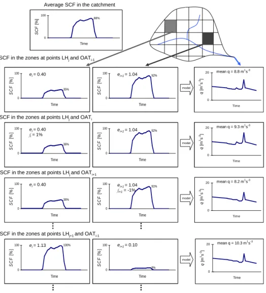
Figure 6.Graph illustrating the spatial LH-OAT SCF sampling for calculating the sensitivity analysis. The top row presents a spatially
averaged observed SCF for an example catchment (top left panel) and the example catchment with highlighted snow zonesiandi+1 (top
right panel). The next rows present SCF in the zonesi(panels in the left column) andi+1 (panels in the central column) in the advancing
LH-OAT loops starting from the loop [i−1, j] and the discharge simulated during these loops (panels in the right column). Symbols are the
same as in Eq. (4):eiandei+1represent a fraction of the SCF in the snow zonesiandi+1,f is the fraction by whichewas changed during
the OAT perturbation,jandj+1 represent the subsequent LH samples,qis the discharge simulated at the catchment outlet.
example of LH-OAT loops for spatial sensitivity analysis de-scribed above is presented in Fig. 6.
The experimental set-up for the spatial sensitivity was as follows. The values of the global parameters of the WetSpa model were the same as those obtained from the model calibration. To be able to achieve convergence, a relatively large number of LH samples was selected (n=100). To-gether with the sample of ei parameters representing 524
4 km×4 km snow zones (p=524), this results in a total number of model evaluations of 52500. The LH samples are taken from a uniform distribution ranging from 0 to 1.14, resulting in a range of 0 to 1 for the SCF in a snow zone (maximum daily mean SCF in the catchment was 88 %; thus
1
0.88 =1.14). The perturbationfi was set to 1 % in order to avoid the OAT samples exceeding the average distance
be-tween the LH samples. The sensitivity analysis was run for 2 full hydrological years from 1 November 2007 to 31 Octo-ber 2009, preceded by a warm-up period of 2 months.
2.4.2 Response functions
Table 1.Descriptions and abbreviations of the 15 response functions (RF) which were used in the sensitivity analysis.
Description RF abbreviation
Yearly Winter Summer
Mean simulated discharge q qw qs
Mean simulated discharge from surface runoff qs qsw qss
Mean simulated discharge from interflow qi qiw qis
Mean simulated discharge from groundwater qg qgw qgs
Mean of the highest 10 % simulated discharges qhigh –
-Mean of the lowest 10% simulated discharges qlow – –
Mean simulated snowmelt vsm – –
the division into winter and summer half-years gives more insight into the seasonal variability of the simulated results. The winter half-year response functions reflect processes occurring during snow accumulation and spring snowmelt when the highest flows occur. However, the summer half-year response functions reflect processes occurring during the summer low flow period. Winter half-year response func-tion were calculated for November until April, summer half-year response function for May until October. Theqhighand qlowreflect processes related to the highest and lowest flows. The vsm is calculated as the mean daily value of snowmelt (mm) and reflects processes related to snowmelt generation without routing.
2.4.3 Output data analysis
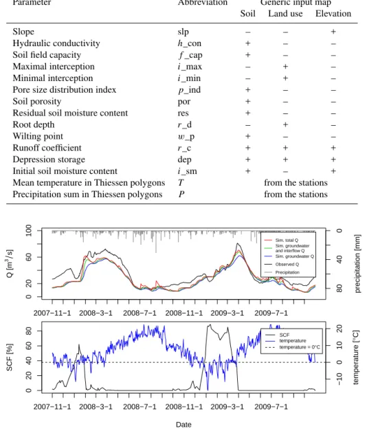
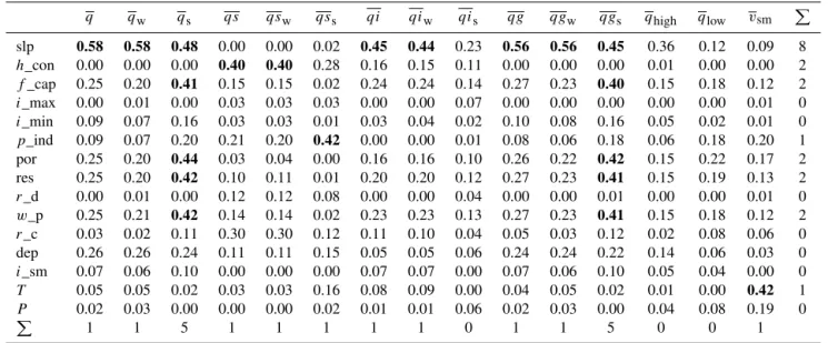
The spatial approach followed in this study gives a large out-put data set, i.e. sensitivity maps based on different response functions. Each sensitivity map was analyzed in light of 15 WetSpa parameter maps presented in Table 2. The Thiessen polygons for potential evapotranspiration were omitted, as there was only one polygon for the whole catchment.
In order to prepare the data set for statistical analysis, each of the 15 parameter maps was spatially aggregated to fit the spatial extent of the sensitivity analysis results (s⋆i) of the
snow zones by calculating the mean (for continuous data) or the majority (for discrete data) of a parameter value in a snow zone. Based on this data set the coefficient of determination (ρ2) was calculated for each pair ofs⋆i and the aggregated
parameter values. Theρ2describes the strength of the linear association between the variables by indicating the fraction of one variable’s variance explained by the second variable. Since in literature the thresholds of ρ2 for quantifying the strength of the linear association are vague, in this paper a ρ2>0.40 is used to represent a moderate association.
3 Results
3.1 Model calibration and performance
The calibrated model shows high efficiencies: NSE=0.86
for the calibration period, NSE=0.73 for the validation
period and NSE=0.79 for the whole period. The
snow-related global WetSpa parameters were estimated dur-ing the calibration as:ksnow= 5.03 mm◦C−1day−1,krain=
0.02 mm mm−1◦C−1day−1. The comparison of observed and simulated discharge is presented in Fig. 7. Of the simu-lated discharge at the catchment outlet, 90 % has a groundwa-ter origin, while surface runoff (5.3 %) and ingroundwa-terflow (4.7 %) contribute mostly to the highest peaks (Fig. 7).
3.2 Spatial sensitivity analysis
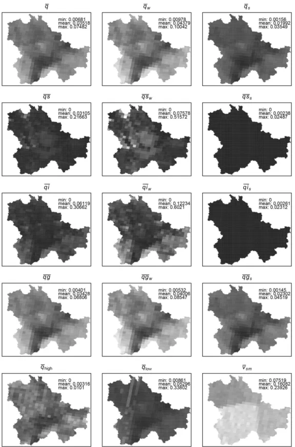
The maps presenting global model output sensitivitiess⋆i to
variations of spatial SCF are presented in Fig. 8. The use of different response function results in different patterns of spatial sensitivity, although some similarities can be distin-guished as well. The minimum, maximum and mean values are indicated on each map (Fig. 8). When the minimum is equal to 0, the model is completely insensitive in at least one snow zone for this response function. The values presented in the first four rows can be compared within a row; however, comparison between the rows is more difficult as in different rows the response functions concern discharge components of different magnitude. Note that the grey scale is different for all maps in the lowest row. This is because, unlike in the upper rows, thes⋆i calculated from these response functions
are not intended to be compared within this row as they con-cern different processes.
Table 2.WetSpa parameter maps used to analyze the sensitivity analysis results: the generic input maps used to derive the parameters maps
are marked with+when used and – when not used.
Parameter Abbreviation Generic input map
Soil Land use Elevation
Slope slp – – +
Hydraulic conductivity h_con + – –
Soil field capacity f_cap + – –
Maximal interception i_max – + –
Minimal interception i_min – + –
Pore size distribution index p_ind + – –
Soil porosity por + – –
Residual soil moisture content res + – –
Root depth r_d – + –
Wilting point w_p + – –
Runoff coefficient r_c + + +
Depression storage dep + + +
Initial soil moisture content i_sm + – +
Mean temperature in Thiessen polygons T from the stations
Precipitation sum in Thiessen polygons P from the stations
2007−11−1 2008−3−1 2008−7−1 2008−11−1 2009−3−1 2009−7−1
0
20
60
100
80
40
0
precipitation [mm]
Q [
m
3
s]
Sim. total Q Sim. groundwater and interflow Q Sim. groundwater Q
Observed Q
Precipitation
2007−11−1 2008−3−1 2008−7−1 2008−11−1 2009−3−1 2009−7−1
0
20
40
60
80
−10
0
10
20
temper
ature [
°
C
]
SCF [%]
Date
SCF temperature temperature = 0°C
Figure 7.Observed and simulated daily discharge from the calibrated WetSpa for the period in which the sensitivity analysis was conducted
(upper panel). Also presented is WetSpa simulated groundwater and interflow discharge as well as only groundwater discharge. Catchment average daily temperature and SCF in the same period is presented in the lower panel. The ticks on the time axis indicate the 1st day of a month.
3.2.1 General relations of the spatial sensitivity
analysis results with parameters maps
The last column of Table 3 shows the frequency of the pa-rameters with moderately strong coefficient of determination under different response functions. The most frequently oc-curring parameter with a coefficient of determination above the threshold (0.40) is slope. The second-most frequent is the group of soil-texture-related parameters: wilting point, hydraulic conductivity, porosity, residual soil moisture and field capacity. The lowest frequency is observed for maximal and minimal interception, initial soil moisture, root depth as
well as parameters responsible for generating surface runoff – runoff coefficient and depression storage.
Figure 8.The SCF sensitivity maps showings⋆i in snow zones of the WetSpa model for Biebrza River catchment for different response
functions. The grey scale represents linearly stretcheds⋆ivalues between minimum (black) and maximum (white); for the top four rows the
Table 3.ρ2values calculated for the WetSpa distributed parameters (rows) and the SCF sensitivity maps under different response functions
(columns).ρ2>0.40 are bold; the frequency that this condition is true is summarized (P
) in the last row and column. Explanation of the response functions and parameters is presented in Tables 1 and 2.
q qw qs qs qsw qss qi qiw qis qg qgw qgs qhigh qlow vsm P
slp 0.58 0.58 0.48 0.00 0.00 0.02 0.45 0.44 0.23 0.56 0.56 0.45 0.36 0.12 0.09 8
h_con 0.00 0.00 0.00 0.40 0.40 0.28 0.16 0.15 0.11 0.00 0.00 0.00 0.01 0.00 0.00 2
f_cap 0.25 0.20 0.41 0.15 0.15 0.02 0.24 0.24 0.14 0.27 0.23 0.40 0.15 0.18 0.12 2
i_max 0.00 0.01 0.00 0.03 0.03 0.03 0.00 0.00 0.07 0.00 0.00 0.00 0.00 0.00 0.01 0
i_min 0.09 0.07 0.16 0.03 0.03 0.01 0.03 0.04 0.02 0.10 0.08 0.16 0.05 0.02 0.01 0
p_ind 0.09 0.07 0.20 0.21 0.20 0.42 0.00 0.00 0.01 0.08 0.06 0.18 0.06 0.18 0.20 1
por 0.25 0.20 0.44 0.03 0.04 0.00 0.16 0.16 0.10 0.26 0.22 0.42 0.15 0.22 0.17 2
res 0.25 0.20 0.42 0.10 0.11 0.01 0.20 0.20 0.12 0.27 0.23 0.41 0.15 0.19 0.13 2
r_d 0.00 0.01 0.00 0.12 0.12 0.08 0.00 0.00 0.04 0.00 0.00 0.01 0.00 0.00 0.01 0
w_p 0.25 0.21 0.42 0.14 0.14 0.02 0.23 0.23 0.13 0.27 0.23 0.41 0.15 0.18 0.12 2
r_c 0.03 0.02 0.11 0.30 0.30 0.12 0.11 0.10 0.04 0.05 0.03 0.12 0.02 0.08 0.06 0
dep 0.26 0.26 0.24 0.11 0.11 0.15 0.05 0.05 0.06 0.24 0.24 0.22 0.14 0.06 0.03 0
i_sm 0.07 0.06 0.10 0.00 0.00 0.00 0.07 0.07 0.00 0.07 0.06 0.10 0.05 0.04 0.00 0
T 0.05 0.05 0.02 0.03 0.03 0.16 0.08 0.09 0.00 0.04 0.05 0.02 0.01 0.00 0.42 1
P 0.02 0.03 0.00 0.00 0.00 0.02 0.01 0.01 0.06 0.02 0.03 0.00 0.04 0.08 0.19 0
P
1 1 5 1 1 1 1 1 0 1 1 5 0 0 1
3.2.2 Discharge source response functions
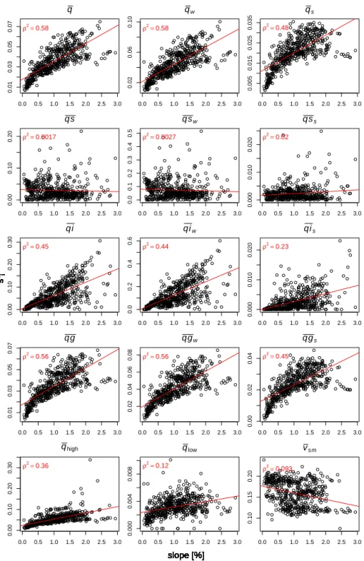
Usingqandqwas response functions resulted in a clear pat-tern differentiating the upland from the valley (cf. Figs. 8 and 5), showing that SCF zones occurring in the flat, organic-soil-dominated valley is much less sensitive than in the min-eral upland. High sensitivity is obtained in snow zones with steeper slopes (cf. Figs. 8 and 2), which is confirmed by highρ2(Table 3). Several WetSpa parameters (mostly soil-texture-dependent: depression storage, wilting point, field ca-pacity, porosity, residual soil moisture content) have highρ2 withqandqwresponse functions (Table 3).
Some differences between q and qs are visible when analysingρ2(Table 3). The SCF sensitivity forqshas higher ρ2for parameters that are related to groundwater flow, like porosity, residual soil moisture content, field capacity and pore size distribution index.
When comparingq,qw andqs toqg,qgw andqgs with respect to spatial patterns (Fig. 8) andρ2(Table 3), the fig-ures are very similar. The group of parameters responsible for groundwater processes (porosity, residual soil moisture content, field capacity and pore size distribution index) have higher ρ2 with the groundwater response functionsqgand qgwthan withq andqw.
The SCF sensitivity forqsandqswdifferentiates the river valley and the north-western upland catchment from the south-eastern upland (cf. Figs. 8 and 5). The maps of SCF sensitivity forqsandqsware the only ones that show clearly a relatively higher sensitivity in the river valley than in most of the upland.
The SCF sensitivity for the interflow response function differs from the groundwater and surface water response
function results. The spatial pattern of SCF sensitivity forqi andqiwseems opposite to the pattern ofqsandqsw.
3.2.3 Extreme discharges response functions
The SCF sensitivity forqhighandqlowpresents a spatial pat-tern that can not be visually related to land-use, soil or slope maps (Fig. 8). These response functions do not correlate with any of the WetSpa spatial parameters (Table 3). The spatial pattern ofqhighshows high values both in the upland and in the valley; however it also has some zones of low sensitivity in the central part of valley. Low but noticeableρ2is found only with the slope. The spatial pattern ofqlow is quite uni-form, with some higher values in the western uplands and lower values in the central part of the valley and in flat re-gions in the northern upland (cf. Figs. 5 and 8).
3.2.4 Mean snowmelt response function
The pattern ofvsmshows random values with different means in different Thiessen polygons for temperature stations used in the model (Fig. 8). This pattern is confirmed by highρ2 betweenvsmand temperature, with no other parameters hav-ing noticeableρ2(Table 3).
4 Discussion
4.1 Model calibration and performance
●● ● ● ● ● ● ● ●● ● ● ● ● ●●● ●●● ● ●● ● ● ●● ● ● ● ● ● ● ●● ● ● ● ● ● ● ● ●● ● ● ● ●● ● ● ● ● ● ● ●● ● ●● ● ● ● ● ● ● ● ● ● ● ● ●● ● ● ● ● ● ● ● ● ● ● ●● ● ● ● ● ● ● ● ●● ● ● ● ● ● ● ● ● ● ● ● ● ● ●● ● ●● ● ● ● ● ● ● ● ● ● ● ● ● ● ● ● ● ● ● ● ● ● ● ● ● ● ● ● ● ● ● ● ● ● ● ● ● ●● ●● ● ●● ● ● ● ● ● ● ● ● ● ● ● ● ● ● ● ● ● ● ● ● ● ●● ● ● ● ● ● ● ●●●● ●● ● ● ●● ● ●●● ● ● ● ●● ● ● ● ● ● ● ● ● ● ● ● ● ● ●● ● ● ● ● ● ●● ● ● ● ●●●●● ●●● ● ● ● ● ●● ●● ● ● ● ● ● ● ● ● ● ● ●●● ● ●● ● ● ● ● ● ●● ●● ● ● ● ● ● ● ● ● ● ● ● ● ●●● ● ● ● ● ● ● ● ● ●● ● ●● ● ● ● ● ● ● ●● ● ● ● ● ●●● ●● ● ● ● ● ●● ●● ●●●●●● ● ● ● ●● ● ● ● ● ● ● ●● ●● ● ●● ● ● ● ●●● ● ● ● ● ● ● ● ● ● ● ● ● ●●● ●● ●● ● ●●● ● ●●●●● ● ●● ● ●● ● ● ● ● ● ● ●●●● ●● ●● ●● ● ● ●● ● ● ● ● ● ● ●● ● ● ●● ● ●● ● ● ● ● ● ● ● ● ● ● ● ●● ● ● ● ● ● ●● ● ● ● ● ●● ● ● ●● ● ● ● ● ● ● ●● ● ●● ● ● ● ● ● ● ● ● ● ● ●● ●● ● ● ● ● ● ● ● ● ● ● ● ●● ●●● ● ● ● ● ● ● ● ● ● ● ● ● ●● ●●● ● ● ● ●● ● ● ● ● ● ● ● ● ●
0.0 0.5 1.0 1.5 2.0 2.5 3.0
0.01 0.03 0.05 0.07 q s* i slope [%]
ρ2=
0.58 ●● ● ● ● ● ● ● ● ● ● ● ● ● ●●● ●●●● ●● ●● ●● ● ● ● ● ● ● ●● ● ●● ●● ● ● ●●● ● ● ● ● ● ● ● ● ● ● ●● ●●● ●● ● ● ● ● ● ● ● ● ● ●●● ● ● ● ● ● ● ● ● ● ●● ● ● ● ● ● ● ● ●● ● ● ● ● ● ● ● ● ● ● ● ● ● ●● ● ●● ● ● ● ● ●● ● ● ● ● ● ● ● ● ● ● ● ● ● ● ● ● ● ● ● ● ● ● ● ● ● ● ● ● ● ● ●● ●● ● ●● ● ● ● ● ● ● ● ● ● ● ● ● ● ● ● ● ● ● ● ● ● ●● ● ● ● ● ● ● ●●● ● ●● ● ● ●● ● ●●●● ● ● ● ● ● ● ● ● ● ● ● ● ● ● ● ● ● ●● ● ● ● ● ● ● ● ● ● ● ●●●●● ●●● ● ● ● ● ●●● ● ● ● ● ● ● ● ● ● ● ● ●●● ● ●● ● ● ● ● ● ●● ●● ● ● ● ● ● ● ● ● ● ● ● ● ●●● ● ● ● ● ● ● ● ● ●● ● ●● ● ● ● ● ● ● ●● ● ● ● ● ●●● ●● ● ● ● ● ●● ●● ●●● ●● ● ● ● ● ●● ● ● ● ● ● ● ●● ●● ●●● ● ● ● ●●● ● ● ● ● ● ● ● ● ● ● ● ● ●●● ●● ●● ● ● ●● ● ●●●●● ● ●● ● ●● ● ● ● ● ● ● ● ● ● ●●● ● ● ●● ● ● ●● ● ● ● ● ●● ●● ● ● ●● ● ●● ● ● ● ● ● ● ● ● ● ● ● ●● ● ● ● ● ● ●● ● ● ● ● ●● ● ● ● ● ● ● ● ●● ● ●● ●●●● ● ● ● ● ● ● ● ● ●●● ●● ● ● ● ● ● ● ● ● ● ● ● ●● ● ●● ● ● ● ● ● ● ● ● ● ● ● ● ●● ● ●● ● ● ● ●● ● ● ● ● ● ● ● ● ●
0.0 0.5 1.0 1.5 2.0 2.5 3.0
0.02 0.06 0.10 qw s* i slope [%]
ρ2=
0.58 ●● ● ● ● ● ● ● ● ● ● ● ● ● ●●● ●●● ● ● ● ● ● ●● ● ● ● ● ● ● ●● ● ● ● ● ● ● ● ● ● ● ● ● ● ● ● ● ● ● ● ● ● ● ● ●● ● ● ● ● ● ● ● ● ● ● ● ●●● ● ● ● ● ● ● ● ● ● ● ●● ● ● ● ●● ● ● ● ●● ● ● ● ● ● ● ● ● ● ● ● ● ● ● ● ● ● ● ● ● ● ● ● ● ● ● ● ● ● ● ● ● ● ● ● ● ● ● ● ● ● ● ● ● ● ● ● ● ● ● ● ● ●● ●● ● ●● ● ● ● ● ● ● ● ● ● ● ● ● ● ● ● ● ● ● ● ● ● ●● ● ● ● ● ● ● ● ● ● ● ●● ● ● ●● ● ● ●● ● ● ● ● ● ● ● ● ●●●● ● ● ● ● ● ● ●● ● ● ● ● ● ● ● ● ● ●●●● ●● ●● ● ● ● ● ● ●● ● ● ● ● ● ● ● ● ● ●● ● ●●● ● ●● ● ● ● ● ● ●● ●●●● ● ● ● ● ● ● ● ●● ● ●●● ● ● ● ● ● ● ● ● ● ● ● ● ● ● ● ● ● ● ● ● ● ● ● ● ● ●●● ● ● ● ● ●● ● ● ●● ● ● ● ●●● ● ● ● ● ● ● ● ● ● ● ● ● ● ● ● ● ● ● ● ● ● ● ● ● ● ● ● ● ● ● ● ● ● ● ● ● ●●● ●● ●● ●● ●● ● ● ●● ●● ● ● ● ● ●● ● ● ● ● ● ● ● ● ● ●●● ●● ● ● ● ●●● ● ● ●● ● ● ●● ● ● ●● ● ●● ● ● ● ●● ● ● ● ● ● ● ● ● ● ● ● ● ● ●● ● ● ● ● ● ●● ● ● ● ● ● ● ● ● ● ●● ● ●● ● ● ● ● ● ● ● ● ● ●● ● ●● ● ● ● ● ● ● ● ● ● ● ● ●●● ●● ● ● ● ● ● ● ●● ●●● ● ●● ●●● ● ● ● ● ● ● ● ● ● ● ● ● ● ●
0.0 0.5 1.0 1.5 2.0 2.5 3.0
0.005 0.015 0.025 0.035 qs s* i slope [%]
ρ2=0.48
●● ● ● ● ● ●●● ● ●●●●●●●● ●●● ●● ● ● ●● ● ● ● ● ● ● ●● ● ●● ●● ● ● ● ● ● ● ● ●● ● ● ● ● ● ● ● ● ●●● ●● ● ● ● ● ● ● ● ● ● ●● ● ● ● ● ● ● ● ● ● ● ●● ● ●●●● ●● ●●● ● ● ● ● ● ● ● ● ● ●● ● ●● ● ● ●●●● ● ●● ● ● ●● ● ● ● ● ● ● ● ● ● ● ● ● ●●●● ● ● ●● ● ● ●● ● ● ●● ●● ●● ● ● ● ● ● ● ● ● ● ●● ● ● ● ● ● ● ● ● ● ● ● ●● ● ● ●● ● ● ● ● ●● ● ● ● ● ● ● ● ● ● ● ● ● ● ●● ● ● ● ● ● ● ● ● ● ● ● ● ● ●● ● ● ● ● ● ● ● ● ● ● ●● ● ● ● ●●● ● ● ● ● ● ● ● ●●●●● ● ● ● ● ● ● ●● ● ●● ● ● ● ● ● ● ● ● ●● ●● ● ● ● ● ● ● ● ● ● ● ●●● ● ● ● ● ● ● ● ● ● ●● ● ● ● ● ● ● ● ● ● ● ● ● ● ● ● ● ●●● ● ● ● ● ● ● ● ● ● ● ● ● ● ●● ● ●●●● ● ● ● ● ● ● ● ● ● ● ● ● ● ●● ●●● ● ● ● ● ● ● ● ● ● ● ● ● ● ● ● ● ● ●● ● ● ● ● ● ● ● ● ●● ● ● ●●● ●● ● ● ● ● ● ● ● ● ● ●● ● ● ● ● ● ●● ● ● ● ●●● ● ●● ● ● ● ● ● ● ● ● ● ● ● ● ● ● ● ● ● ● ● ● ● ● ● ●●●●● ● ● ● ● ● ● ● ●● ● ● ● ● ● ● ● ● ● ● ● ● ● ● ● ● ● ● ● ● ● ● ● ● ● ● ● ● ● ● ● ● ● ● ● ● ●● ●● ● ● ● ● ● ● ● ● ● ● ● ● ● ●● ● ● ● ● ● ● ● ● ● ● ● ● ● ● ● ● ●
0.0 0.5 1.0 1.5 2.0 2.5 3.0
0.00 0.10 0.20 qs s* i slope [%]
ρ2=
0.0017 ●● ● ● ● ● ●●● ● ●●●●●●●● ●●● ●● ●● ●● ● ● ● ● ● ● ●● ● ●● ●● ● ● ● ● ● ● ● ●● ● ● ● ● ● ● ● ● ●●● ●●●● ● ● ● ● ● ● ● ●● ● ● ● ● ● ● ● ● ● ● ●● ● ●●●● ●● ●●● ● ● ● ● ● ● ● ● ● ●● ● ●● ● ● ●●●● ● ●● ● ● ●● ● ● ● ● ● ● ● ● ● ● ● ● ●●●● ● ● ●● ● ● ●● ● ● ●● ●● ●● ● ● ● ● ● ● ● ● ● ●● ● ● ● ● ● ● ● ● ● ● ● ●● ● ● ●● ● ● ● ● ●● ● ● ● ● ● ● ● ● ● ● ● ● ● ● ● ● ● ● ● ● ● ● ● ● ● ● ● ● ●● ● ● ● ● ● ● ● ● ● ● ●● ● ● ● ●●● ● ● ● ● ● ●● ●●●●● ● ● ● ● ● ● ●● ● ●● ● ● ● ● ● ● ● ● ●● ●● ● ● ● ● ● ● ● ● ● ● ●●● ● ● ● ● ● ● ● ● ● ●● ● ● ● ● ● ● ● ● ● ● ● ● ● ● ● ● ●●● ● ●● ● ● ● ● ● ● ● ● ● ● ●● ● ●●● ● ● ● ● ● ● ● ● ● ● ● ● ● ● ●● ●●● ● ● ● ● ● ● ● ● ● ● ● ● ● ● ● ● ● ●● ● ● ● ● ● ● ● ● ●● ● ● ● ●●●● ● ● ● ● ● ● ● ● ● ●● ● ● ● ● ● ●● ● ● ● ●●● ● ●● ● ● ● ● ● ● ● ● ● ● ● ● ● ● ● ● ● ● ● ● ● ● ● ●●●●● ● ● ● ● ● ● ● ●● ● ● ● ● ● ● ● ● ● ● ● ● ● ● ● ● ● ● ● ● ● ● ● ●● ● ● ● ● ● ● ● ● ● ● ● ●●●● ● ● ● ● ● ● ● ● ● ● ● ● ● ●● ● ● ● ● ● ● ● ● ● ● ● ● ● ● ● ● ●
0.0 0.5 1.0 1.5 2.0 2.5 3.0
0.0 0.1 0.2 0.3 0.4 0.5 qsw s* i slope [%]
ρ2=
0.0027 ●● ● ● ● ● ●●● ● ●●●●●●●●●●● ●● ● ● ●● ● ● ● ● ● ● ●● ● ● ● ● ● ● ● ●●●● ● ●● ● ● ● ● ● ● ● ● ●●● ●●●● ● ● ● ● ● ● ● ●● ● ● ● ● ● ● ● ● ● ● ●● ● ●●●●● ●●●●●●●● ● ● ● ● ● ●●● ●●● ●● ● ● ● ● ● ● ● ● ●● ● ● ●● ● ● ● ● ● ● ● ● ●● ●● ● ● ●● ● ● ●● ● ● ●● ●●●● ● ● ● ● ● ● ● ● ● ●● ● ● ● ●●●● ● ● ● ● ●● ● ● ● ●● ●● ● ● ● ● ● ● ● ●● ● ● ● ● ● ● ● ●● ● ● ● ● ●●● ●●● ● ● ● ●● ● ● ●● ● ●● ● ● ● ● ● ● ● ● ●●● ● ● ● ● ● ● ●●●●●●● ● ●● ● ● ●● ● ● ● ● ● ● ● ● ● ● ● ●● ●● ● ● ● ● ● ● ● ●● ● ●●● ● ● ● ● ● ● ● ● ● ●● ● ● ● ● ● ● ● ● ● ● ● ● ● ● ● ● ● ● ● ● ●●● ● ● ● ● ●●●●●● ● ● ● ● ●● ● ● ● ● ● ● ● ● ● ● ●● ● ●● ●●● ●●● ● ● ● ● ● ● ● ● ● ●● ●● ● ●● ● ● ● ● ● ● ● ● ●● ● ●●●●●●● ● ● ● ● ● ● ● ● ● ● ● ● ● ● ● ●● ● ●● ● ● ●●● ●● ● ● ● ● ● ● ● ● ● ● ● ● ● ● ● ● ● ●● ● ● ● ●●●●● ● ● ● ● ● ● ● ●● ● ● ●●●● ●● ●● ●● ● ● ● ● ● ● ● ● ● ● ● ● ● ● ● ● ● ● ● ● ● ● ● ● ● ● ●● ● ● ● ● ● ● ● ● ● ● ● ● ● ●● ● ● ● ● ● ● ● ● ● ● ● ● ● ● ● ● ●
0.0 0.5 1.0 1.5 2.0 2.5 3.0
0.000 0.010 0.020 qss s* i slope [%]
ρ2=
0.02 ●● ● ● ● ● ● ● ● ● ● ●● ● ●● ● ●●●● ●● ● ● ● ● ● ● ● ● ● ● ●● ● ● ● ● ●● ● ● ● ● ● ● ● ● ● ● ● ● ● ● ● ● ●●● ● ● ● ● ● ● ● ● ● ● ●● ●●● ● ● ● ● ● ● ● ● ●● ● ● ● ● ●● ● ●● ● ● ● ● ● ● ● ● ● ● ●● ● ● ● ● ● ● ● ● ● ● ● ● ● ● ● ● ● ● ● ● ● ● ● ● ● ● ● ● ● ● ● ● ● ● ● ● ● ● ●● ● ● ● ● ●● ● ● ● ● ● ● ● ● ● ● ● ● ● ● ● ● ● ● ● ● ● ● ● ● ●● ● ● ● ● ● ● ● ● ●● ●● ● ● ●● ● ● ●●● ● ● ● ● ● ● ● ● ● ● ● ●●● ● ● ● ●● ● ●● ● ● ●● ● ● ●● ● ● ●● ●● ● ● ● ● ● ●●●● ● ●●● ● ●●●●● ●●● ●●● ● ● ● ● ● ●● ●●●●● ● ● ● ● ● ● ●● ● ●●● ● ● ● ● ● ● ● ● ●● ● ●● ● ● ● ● ● ● ● ● ● ● ● ● ●●● ●● ● ● ●●● ● ●●● ● ● ● ● ●● ● ● ● ● ● ● ● ● ● ● ● ● ● ● ●● ● ● ●● ●●● ● ● ● ● ● ● ● ● ● ● ● ● ●● ● ● ● ●● ●● ● ● ● ● ● ● ●● ●●● ● ● ● ● ● ● ● ● ● ● ● ● ● ● ● ● ● ● ● ● ●●● ● ● ●● ● ● ● ● ● ● ● ● ● ●● ● ● ● ● ● ● ● ● ● ● ● ● ● ● ● ● ● ● ●● ● ● ● ● ● ● ● ● ● ● ● ● ● ● ● ● ● ● ● ●● ● ● ● ● ● ● ● ● ● ●● ● ● ● ● ● ● ● ● ● ● ● ● ● ● ●● ● ●● ● ● ● ● ● ● ● ● ● ● ● ● ●● ● ●● ● ● ● ●● ● ● ● ● ● ● ● ● ●
0.0 0.5 1.0 1.5 2.0 2.5 3.0
0.00 0.10 0.20 0.30 qi s* i slope [%]
ρ2=0.45
●● ● ● ● ● ● ● ● ● ● ●● ● ●● ● ●● ●● ●● ● ● ● ● ● ● ● ● ● ● ●● ● ● ● ● ●● ● ● ● ● ● ● ● ● ● ● ● ● ● ● ●● ●●● ● ● ● ● ● ● ● ● ● ● ●● ●●● ● ● ● ● ● ● ● ● ●● ● ● ● ● ●● ● ●● ● ● ● ● ● ● ● ● ● ● ●● ● ● ● ● ● ● ● ● ● ● ● ● ● ● ● ● ● ● ● ● ● ● ● ● ● ● ● ● ● ● ● ● ● ● ● ● ● ● ●● ● ● ● ● ●● ● ● ● ● ● ● ● ● ● ● ● ● ● ● ● ● ● ● ● ● ● ● ● ● ●● ● ● ● ● ● ● ● ● ●● ●● ● ● ●● ● ●●●● ● ● ● ● ● ● ● ● ● ● ● ●●● ● ● ● ●● ● ●● ● ● ●● ● ● ●● ● ●●● ●● ● ● ● ● ● ●●●● ● ●●● ● ●● ●● ● ●●●● ●● ● ● ● ● ● ●● ●●●●● ● ● ● ● ● ● ●● ● ●●● ● ● ● ● ● ● ● ● ●● ● ●● ●● ● ● ● ● ● ● ● ● ● ● ●●● ●● ● ● ●●● ● ●● ● ● ● ● ● ●● ● ● ● ●● ● ● ● ● ● ● ● ● ● ●● ● ● ● ● ●●● ● ● ● ● ● ● ● ● ● ● ● ● ●● ● ● ● ●● ●● ● ● ● ● ● ● ●● ●●● ● ● ● ● ● ● ● ● ● ● ● ● ● ● ● ● ● ● ● ● ●●● ● ● ●● ● ● ● ● ● ● ● ● ● ●●● ● ● ● ● ● ● ● ● ● ● ●● ● ● ● ● ● ●● ● ● ● ● ● ● ● ● ● ● ● ● ● ● ● ● ● ● ● ●● ● ● ● ● ● ● ● ● ● ●● ● ● ● ● ● ● ● ● ● ● ● ● ● ● ●● ● ●● ● ● ● ● ● ● ● ● ● ● ● ● ●● ● ●● ● ● ● ●● ● ● ● ● ● ● ● ● ●
0.0 0.5 1.0 1.5 2.0 2.5 3.0
0.0 0.2 0.4 0.6 qiw s* i slope [%]
ρ2=0.44
●● ● ● ● ● ● ● ● ● ● ●● ● ● ● ● ● ● ● ● ●● ●● ● ● ● ● ● ● ● ● ●● ● ● ● ● ● ● ● ● ● ● ● ● ● ● ● ● ● ● ● ● ●● ● ● ● ● ● ● ● ● ● ● ● ● ● ●● ● ● ● ● ● ● ● ● ● ● ● ●●● ● ● ●● ● ● ●● ● ● ● ● ● ● ● ● ● ● ●● ● ● ● ● ● ● ● ● ● ● ● ● ● ● ● ● ● ● ●● ● ● ● ● ● ● ● ● ● ● ● ● ● ●●● ● ● ●● ● ● ● ● ●● ● ● ● ● ● ● ● ● ● ● ● ● ● ● ● ● ● ● ● ● ● ● ● ● ●● ● ● ● ● ● ● ● ● ●● ●● ● ● ●● ● ● ●●● ● ● ● ● ● ● ● ● ● ● ● ●●●●● ● ●● ● ● ● ● ● ● ● ● ● ●● ● ● ●● ●●● ● ● ● ● ●●●● ●●●●● ● ● ● ● ● ● ●●●●● ● ● ● ● ● ●●●●●●●● ● ● ● ● ● ● ● ● ● ●● ● ● ● ● ● ● ● ● ●●●●●●● ● ● ● ● ●● ● ● ● ● ● ●● ● ● ● ● ●●● ● ● ●●●●●●●● ●● ● ●● ● ● ● ● ● ●● ● ● ● ● ● ● ● ● ● ● ● ● ● ● ● ●● ● ● ● ● ● ● ● ● ● ● ● ● ● ● ● ● ● ● ●● ● ●● ● ●●●●●● ● ● ● ● ● ● ● ● ● ● ● ● ● ● ● ● ●● ●●●●●●● ●● ● ● ● ● ● ●● ● ● ● ● ● ● ● ● ● ● ● ● ● ● ● ● ●●●● ● ● ● ● ● ● ● ● ● ● ● ● ● ●● ● ● ● ● ● ● ● ● ● ● ● ● ● ● ● ● ● ● ● ● ● ● ● ● ● ● ● ● ● ● ● ● ● ● ● ● ● ● ● ● ● ● ● ● ● ● ● ● ● ● ● ●● ● ● ● ● ● ● ● ● ● ● ● ● ● ●
0.0 0.5 1.0 1.5 2.0 2.5 3.0
0.000 0.010 0.020 qis s* i slope [%]
ρ2=0.23
●● ● ● ● ● ● ● ●● ● ● ● ● ●●● ● ●● ● ●● ● ● ●● ● ● ● ● ● ● ●● ● ● ● ● ● ● ● ●● ● ● ● ●● ● ● ● ● ● ● ●● ● ●● ●● ● ● ● ● ● ● ● ● ● ●● ● ● ● ● ● ● ● ● ● ● ●● ● ● ● ● ● ● ● ●● ● ● ● ● ● ● ● ● ● ● ● ● ● ● ● ● ●● ● ● ● ● ● ● ● ● ● ● ● ● ● ● ● ● ● ● ● ● ● ● ● ● ● ● ● ● ● ● ● ● ● ● ● ● ●● ●● ● ●● ● ● ● ● ● ● ● ● ● ● ● ● ● ● ● ● ● ● ● ● ● ●● ● ● ● ● ● ● ● ● ● ● ●● ● ● ●● ● ● ●● ● ● ● ●● ● ● ● ●●●● ● ● ● ● ● ● ●● ● ● ● ● ● ●● ● ● ● ●●●●● ●●● ● ● ● ● ●● ● ● ● ● ● ● ● ● ●● ● ● ●●● ● ●● ● ● ● ● ● ●● ●● ● ● ● ● ● ● ● ● ● ● ● ● ●●● ● ● ● ● ● ● ● ● ●● ● ●● ● ● ● ● ● ● ● ● ● ● ● ● ●●● ●● ● ● ● ● ● ● ● ● ● ● ● ●● ● ● ● ● ●● ● ● ● ● ● ● ●● ●● ●●● ● ● ● ● ● ● ● ● ● ● ● ● ● ● ● ● ● ● ●●●●● ●● ●●●● ● ● ●● ●● ● ● ● ● ● ● ● ● ● ● ● ● ● ●● ● ● ● ● ● ● ● ● ● ● ● ● ● ● ● ●● ●● ● ● ●● ● ●● ● ● ● ●● ● ● ● ● ● ● ● ● ● ● ● ● ● ●● ● ● ● ● ● ● ● ● ●● ● ● ● ●● ● ● ● ● ●● ● ● ● ● ● ● ● ● ● ● ● ● ●● ● ● ● ● ● ● ● ● ● ● ● ●●●●● ● ● ● ● ● ● ● ● ● ● ● ● ●● ● ●● ● ● ● ● ● ● ● ● ● ● ● ● ● ●
0.0 0.5 1.0 1.5 2.0 2.5 3.0
0.01 0.03 0.05 0.07 qg s* i slope [%]
ρ2=0.56
●● ● ● ● ● ● ● ● ● ● ● ● ● ●●● ●●● ● ●● ●● ●● ● ● ● ● ● ● ●● ● ● ● ● ● ● ● ●● ● ● ● ●● ● ● ● ● ● ● ●● ●● ● ●● ● ● ● ● ● ● ● ● ● ●●● ● ● ●●● ● ● ● ● ●● ● ● ● ● ● ● ● ●● ● ● ● ● ● ● ● ● ● ● ● ● ● ●● ● ●● ● ● ● ● ● ● ● ● ● ● ● ● ● ● ● ● ● ● ● ● ● ● ● ● ● ● ● ● ● ● ● ● ● ● ● ● ●● ●● ● ●● ● ● ● ● ● ● ● ● ● ● ● ● ● ● ● ● ● ● ● ● ● ●● ● ● ● ● ● ● ●●● ● ●● ● ● ●● ● ● ●● ● ● ● ● ● ● ● ● ●●●● ● ● ● ● ● ● ●● ● ● ● ● ● ● ● ● ● ● ●●● ● ● ●●● ● ● ● ● ●● ● ● ● ● ● ● ● ● ●● ● ● ●●● ● ●● ● ● ● ● ● ●● ●● ● ● ● ● ● ● ● ● ● ● ● ● ●●● ● ● ● ● ● ● ● ● ●● ● ●● ● ● ● ● ● ● ● ● ● ● ● ● ●●● ●● ● ● ● ● ● ● ●● ● ● ● ●● ● ● ● ● ●● ● ● ● ● ● ● ●● ●● ●●● ● ● ● ●●● ● ● ● ● ● ● ● ● ● ● ● ● ●●●●● ●● ●●●● ● ● ●● ●● ● ●● ● ●● ● ● ● ● ● ● ● ● ● ● ● ● ● ● ●● ● ● ● ● ● ● ● ●● ● ● ● ● ● ●● ● ●● ● ● ● ●● ● ● ● ● ● ● ● ● ● ● ● ● ● ●● ● ● ● ● ● ● ● ● ● ● ● ● ● ● ● ● ● ● ● ●● ● ● ● ● ● ● ● ● ● ●● ● ● ● ● ● ● ● ● ● ● ● ● ● ● ●●●●● ● ● ● ● ● ● ● ● ● ● ● ● ●● ● ● ● ● ● ● ● ● ● ● ● ● ● ● ● ● ●
0.0 0.5 1.0 1.5 2.0 2.5 3.0
0.02 0.04 0.06 0.08 qgw s* i slope [%]
ρ2=0.56
●● ● ● ● ● ● ● ● ●● ●● ● ●● ● ●●● ● ● ● ● ● ● ● ● ● ● ● ● ● ●● ● ● ● ● ● ● ● ● ● ● ● ● ● ● ● ● ● ● ● ● ● ● ● ●● ● ● ● ● ● ● ● ● ● ● ● ● ● ● ● ● ● ● ● ● ● ● ● ● ● ● ● ● ● ●● ● ● ● ●● ● ● ● ● ● ● ● ● ● ● ● ● ● ● ● ● ● ● ● ● ● ● ● ● ● ● ● ● ● ● ● ● ● ● ● ● ● ● ● ● ● ● ● ● ● ● ● ● ● ● ● ● ●● ●●●●● ● ● ● ● ● ● ● ● ● ● ● ● ● ● ● ● ● ● ● ● ● ●● ● ● ● ● ● ● ● ● ● ● ●● ● ● ●● ● ● ● ● ● ● ● ● ● ● ● ● ●●●● ● ● ● ● ● ● ●● ● ● ● ● ● ● ● ● ● ●●●● ●● ●● ● ● ● ● ● ●● ● ● ● ● ● ● ● ● ● ●● ● ●●● ● ●● ● ● ● ● ● ●● ●●●● ● ● ● ● ● ● ● ●● ● ●●● ● ● ● ● ● ● ● ● ● ● ● ● ● ● ● ● ● ● ● ●● ● ● ● ● ●●●●● ● ● ●● ● ● ●● ● ● ● ●●● ● ● ● ● ● ● ● ● ● ● ● ● ● ● ● ●● ● ● ● ● ● ● ● ●●● ● ● ● ● ● ● ● ● ● ●●● ●● ●● ● ● ●● ● ● ●● ●● ●● ● ● ●● ● ● ● ● ● ● ● ● ● ● ● ● ● ● ● ● ● ●●● ● ● ●● ● ● ●● ● ● ●● ● ● ● ● ● ● ●● ● ● ● ● ● ● ● ● ● ● ● ● ● ●● ● ● ● ● ●●● ● ● ● ● ● ● ● ● ● ●● ● ●● ● ● ● ● ● ● ● ● ● ●● ● ●● ● ● ● ● ● ● ● ● ● ● ● ●●● ●● ● ● ● ● ● ● ● ● ● ● ● ● ●● ●●● ● ● ● ●● ● ● ● ● ● ● ● ● ●
0.0 0.5 1.0 1.5 2.0 2.5 3.0
0.00 0.02 0.04 qgs s* i slope [%]
ρ2=
0.45 ●● ● ● ● ● ● ● ●● ● ●● ● ●● ●●●● ● ●●●●● ●● ● ●●●●●●● ●● ●● ● ● ●● ● ● ● ●● ● ● ● ● ● ● ●● ●●● ● ●●● ● ● ● ● ● ● ●●● ● ● ●●●●● ● ● ● ●●● ●● ● ●● ● ●●● ●●●● ● ● ● ● ● ●●●● ●●●●●●●● ●● ● ● ● ● ● ● ●● ● ● ● ● ● ● ● ● ●●●● ● ● ●● ● ● ● ● ● ● ●● ●●●●●● ● ● ● ● ● ● ● ● ● ● ● ● ●●●● ● ● ● ● ●● ● ● ●● ● ● ●●●● ●● ● ● ●● ● ● ●●● ● ● ●● ● ●●●●●●●●●●●● ●● ● ●● ●● ● ● ● ●●●●●●●●● ●● ● ● ● ●●●●● ●● ● ● ● ● ●● ● ●●●● ●● ● ● ● ● ● ●●●●●●●● ● ● ● ● ● ● ● ● ●●● ● ● ● ● ● ● ● ● ●●●●●●● ● ● ● ● ●● ● ● ● ● ●●● ●●● ● ●●● ● ● ●●●● ●● ●● ● ● ● ●● ● ● ● ● ● ● ● ● ● ● ● ● ● ●● ●●●● ● ● ● ● ● ● ● ● ● ● ● ●●● ●● ●● ● ● ● ● ● ● ● ● ● ● ● ●● ● ●● ● ● ● ● ● ● ●●●● ●● ●● ● ● ● ●●● ● ● ● ●● ● ●● ● ● ●● ● ●● ● ● ●●●● ● ● ● ● ● ● ● ● ● ●● ●●●●● ● ●●● ●●●● ● ● ● ● ● ● ●● ● ● ● ● ● ● ● ● ● ● ● ● ● ●● ● ● ● ● ● ● ● ● ●●● ● ●●●●●●● ● ● ● ● ● ● ● ● ● ● ● ●●● ●● ●●●●●● ●● ● ● ● ● ● ●
0.0 0.5 1.0 1.5 2.0 2.5 3.0
0.00 0.10 0.20 0.30 qhigh s* i slope [%]
ρ2=
0.36 ● ● ● ● ● ● ● ● ● ●● ● ● ● ●● ● ● ● ● ● ● ● ● ● ● ● ● ● ●●● ● ● ● ● ● ● ● ● ● ● ● ● ● ● ● ●● ● ● ● ● ● ● ● ● ●●● ● ● ● ● ● ● ● ● ● ● ● ● ● ● ● ● ● ● ● ● ● ● ● ● ● ● ● ● ● ● ● ● ● ● ● ● ● ●● ● ● ● ● ● ● ● ● ● ● ● ● ● ● ● ● ● ● ● ● ● ● ● ● ● ●● ● ● ● ● ● ● ● ● ● ● ● ● ● ●●● ● ● ●● ● ● ●● ●● ● ●● ● ● ● ● ● ● ● ● ● ● ● ● ● ● ● ● ● ● ● ● ● ● ● ● ● ● ● ● ● ● ● ●● ●● ● ● ●● ● ●● ● ● ● ● ● ● ● ● ●●●●●●● ● ● ● ● ●● ● ● ● ● ● ● ● ● ● ● ●●● ● ● ● ● ● ● ● ● ● ● ●●● ● ● ● ● ● ● ●● ● ● ●●● ● ●● ● ● ● ● ● ● ●● ● ●● ● ● ● ● ● ● ● ● ● ● ● ● ● ● ● ● ● ● ● ● ● ● ● ● ●● ● ● ● ● ● ● ● ● ● ● ● ● ● ● ●● ● ● ● ● ● ●● ● ● ● ● ● ● ● ● ● ● ● ● ● ● ● ● ● ● ● ●● ● ● ●● ● ● ● ● ● ● ● ●● ● ● ●● ● ● ● ● ● ● ●●●● ● ● ● ● ● ●● ● ●● ● ●● ●● ●● ● ● ● ● ● ● ● ●● ● ● ● ● ● ● ● ●● ● ● ● ● ●●●●● ● ●● ● ● ●● ● ● ● ● ● ●●●● ● ● ● ● ● ● ● ● ● ● ●●●●● ● ● ● ● ● ● ● ●● ● ● ● ●● ● ● ● ● ●● ● ● ● ● ● ● ● ● ● ● ● ● ● ● ● ● ● ● ● ● ● ● ● ● ● ●● ● ● ● ● ● ● ● ● ● ●● ● ● ● ● ●● ●●● ● ● ● ● ● ● ● ● ● ● ● ● ● ●
0.0 0.5 1.0 1.5 2.0 2.5 3.0
0.000 0.004 0.008 qlow s* i slope [%]
ρ2=0.12
● ● ● ● ● ● ● ● ●● ● ● ● ● ●● ● ● ●● ● ● ● ● ● ● ● ● ●● ● ●●●● ● ● ● ● ● ● ● ●● ● ● ● ●● ● ● ● ● ● ● ●● ● ●● ● ●● ● ● ● ● ● ● ● ●●● ● ● ● ●●● ● ● ● ● ●● ● ●●● ●● ●● ● ● ● ● ● ● ● ● ● ● ● ●● ● ● ● ● ●● ● ● ● ● ● ● ● ●●●●●●● ● ● ● ● ● ● ● ● ●● ●● ● ● ● ● ● ● ●● ● ● ●● ● ● ● ● ● ● ● ● ● ● ● ● ● ● ● ● ● ● ● ● ● ● ● ● ● ● ●● ● ● ● ● ● ● ● ● ● ● ● ● ● ● ●● ● ● ● ● ● ● ● ●● ● ● ● ●●●● ● ● ● ● ● ● ●● ● ●● ●● ●● ● ● ●●●● ● ● ●●● ● ● ● ● ● ● ● ● ●●● ● ● ● ● ●●● ● ●● ● ●● ● ● ● ● ● ●●● ● ●● ● ● ● ● ● ● ● ● ● ● ●●● ● ● ● ● ● ● ● ● ● ● ● ●● ● ● ● ● ● ● ●● ● ● ● ● ●●● ● ● ● ● ● ● ● ● ● ●● ● ● ●●● ● ●● ● ● ● ● ● ● ● ● ● ● ● ● ● ● ● ● ●● ● ● ● ● ● ● ● ●● ● ● ● ● ● ● ●●●●● ●● ● ● ● ● ● ●●●●● ● ● ● ● ● ● ● ● ● ● ● ●●● ●●● ● ● ● ●● ● ●● ● ●●●●● ● ●● ● ● ●● ● ● ● ● ● ●●●● ● ● ● ● ● ● ● ● ● ● ● ● ●● ● ● ● ● ●● ● ● ●● ● ● ● ● ● ● ●● ● ● ● ● ● ● ● ● ● ● ● ● ● ● ● ● ● ● ● ● ● ● ● ● ● ● ● ● ● ● ●●● ● ● ● ● ●●●●● ● ● ●●● ●●● ●● ● ●●●● ● ● ● ● ● ● ●
0.0 0.5 1.0 1.5 2.0 2.5 3.0
0.10 0.15 0.20 vsm s* i slope [%]
ρ2=
0.093
Figure 9.Relation between the slope and spatial sensitivity analysis results (s⋆i) quantified with different response functions. Explanation of
the response functions is presented in Table 1.
underestimated by 8 % of the observed value on average. The underestimations of peak discharges are possibly de-termined by the uncertainty of the rating curve. During the yearly spring floods, the measurement profile near the gaug-ing station widens outside the riverbed and extends into the densely vegetated floodplain, where proper hydraulic mea-surements are very difficult. Nonetheless, the shape of the