Braz. J. Chem. Eng. vol.32 número2

ISSN 0104-6632 Printed in Brazil

www.abeq.org.br/bjche

Vol. 32, No. 02, pp. 531 - 542, April - June, 2015 dx.doi.org/10.1590/0104-6632.20150322s00003300

Brazilian Journal

of Chemical

Engineering

INFLUENCE OF INTERFACIAL FORCES ON THE

MIXTURE PREDICTION OF AN ANAEROBIC

SEQUENCING BATCH REACTOR (ASBR)

L. M. Rosa

,

G. Z. Maurina

, L. L. Beal

, C. Baldasso

, A. P. Torres

and M. P. Sousa

1_{Laboratory of Environmental Technology, University of Caxias do Sul,}

1130 Francisco Getúlio Vargas St., Caxias do Sul - RS, Brazil. Phone: + (55) (54) 3218 2100

E-mail: [email protected]

2_{CENPES, Petrobras, 950 Horácio Macedo Avenue, Rio de Janeiro - RJ, Brazil.}

(Submitted: February 14, 2014 ; Revised: June 30, 2014 ; Accepted: July 2, 2014)

Abstract - In the operation of bioreactors, the fluid movement promotes mixing between sludge and substrate. The dynamics of this system are complex, and the interaction between the phases is difficult to evaluate accurately. In this work, Computational Fluid Dynamics is applied to simulate a pilot-scale anaerobic sequencing batch reactor, using a three-dimensional, transient and multiphase modeling. Several correlations were applied to estimate the interfacial forces. Results indicate that the use of different coefficients for the drag and lift forces strongly affects the predicted turbulent kinetic energy, and thus the mixture estimation in the bioreactor. The use of the drag as the only interfacial force provided an average turbulent kinetic energy close to the value found using a more complete model. However, the absence of lift and virtual mass forces had a significant impact on the resulting turbulence distribution.

Keywords: Computational fluid dynamics; Interfacial forces; Anaerobic sequencing batch reactor.

INTRODUCTION

Environmental issues cause great concern today. The consumption of fossil fuels is one of the factors that contribute to the greenhouse effect, due to the amount of carbon dioxide that is released into the at-mosphere during the combustion of these fuels. This has motivated the search for new non-polluting fuels, including methane and biohydrogen.

Hydrogen is known to be a clean and ideal energy source due to its renewable status and green effect on the global environment (Nurtono et al., 2012). It can be obtained through physicochemical and biological routes. The hydrogen produced by microorganisms (biohydrogen) is affected simultaneously by biologi-cal, physibiologi-cal, and chemical factors (Ding et al., 2010;

Wang et al., 2009; Wang et al., 2010). One of the most applied approaches for biohydrogen production in-volves the use of anaerobic sequencing batch reac-tors (ASBR), which also benefit the environment by consuming agro-industrial wastes.

be-Brazilian Journal of Chemical Engineering tween the phases promotes contact between the

mi-croorganisms and the substrate, and enhances the production of biogas in the form of bubbles dis-persed through fermentation reactions.

The mixture is promoted by the fluid movement within the reactor, subjected to numerous interac-tions between gas, liquids and solids. The dynamics of this multiphase mixture are complex, and the evaluation of the interaction between phases is chal-lenging. Nonetheless, it is needed to predict the physi-cal characteristics of bioreactors, which are seldom well described (Cao et al., 2010).

In this sense, computational fluid dynamics (CFD) tools can be valuable to study the fluid dynamics in bioreactors, as it provides estimatives of velocity and turbulence intensity in any location inside the reac-tor. However, there are difficulties when simulating the interaction between the disperse gas and the continuous liquid phases, which is affected by inter-facial forces (drag, lift and virtual mass forces). Mul-tiphase modeling relies on various correlations to predict the interaction between the phases, and the difference among the estimated forces can affect the fluid dynamics. The estimated drag and lift force coefficients can vary significantly, depending on the operating conditions and on the correlation con-sidered (Pang and Wei, 2011), leading to differences of the simulated results. It has been found that the magnitude of the drag force is more than 100 times higher than the magnitude of other interfacial forces (Laborde-Boutet et al., 2009). Still, forces such as lift and virtual mass can also play an important role in the motion of bubbles under the normal gravity condition (Pang et al., 2010).

Therefore, the correct modeling of these forces is of prime importance for capturing the physics cor-rectly (Tabib et al., 2008). Nevertheless, the lift force model has not been well established yet (Hibiki and Ishii, 2007). Despite a large number of correlations which disregard the influence of the shear rate on the lift force coefficient estimation, it was found recently that this influence is strong (Dijkhuizen et al., 2010).

The present work uses CFD techniques to deter-mine the influence of drag, lift and virtual mass forces on the behavior of a gas-liquid flow in an ex-isting pilot-scale ASBR, which runs under operating conditions typically found in fermentative processes. The simulated bioreactor has a capacity of 1 m³, operating with a mixture of wastewater and biomass for biohydrogen production. It features asymmetries not commonly found in traditional bubble columns. As mixture is an important parameter in the design of bioreactors, the turbulent kinetic energy predicted from the use of different models is evaluated.

METHODOLOGY

Mathematical Modeling

Three-dimensional transient simulations were car-ried out to predict the fluid dynamics of the proposed cases. The two-fluids approach was applied to resolve the flow of two Eulerian, interpenetrating phases. The phases considered were: (1) a continuous liquid mix-ture and (2) gas bubbles. The formulation described by Weller (2002) apud Rusche (2002) for the incom-pressible two-phase flow equations was adopted. The equations of continuity and momentum transport are presented in Equations (1) and (2), respectively:

( ) (

)

(

(

)

)

∂ _{∇ ∇ −}

∂ (1)

( )

( )

( )

i i i i i

i

i

i i i

α

U +U U + R + R

t α

p M

= + g +

ρ α ρ

∂ _{∇ ∇} ∇

∂ ∇ −

(2)

where the index i represents the phase (“g” stands for gas, “l” for liquid). Ui represents the velocity of the phase, Ur is the relative velocity between the phases,

i

α is its volume fraction, g is the gravity accelera-tion, p is the pressure, ρ_i is the phase density, and M_i represents the momentum transfer between the phases due to interfacial forces. Where α_i appears in the de-nominator, it is summed with a small value to avoid numerical errors. R_ieff represents the stress tensor, re-lated to viscous forces, and is defined in Equation (3):

(

)

. 0

3 3

eff eff T

i i i i

i i

R =−υ ⎛_⎜∇U + ∇U − I∇U + I k =⎞_⎟

⎝ ⎠ (3)

where I is a unit tensor, υ_ieff is the effective viscosity, and k_i is the turbulent kinetic energy of the phase i. The k-ε turbulence model was used to determine the influence of turbulence in the liquid phase. It consid-ers the Boussinesq assumption, in which the effec-tive continuous phase viscosity is given by the sum of the laminar viscosity υ_l and the eddy viscosity υt, which is defined in Equation (4):

2

( / )

t

μ l l

υ = C k ε (4)

( ) (

)

eff l

l l l l k l

k

υ

k + U k k P ε

t σ

⎛ ⎞

∂ _{∇ − ∇ ∇ = −}

⎜ ⎟

⎜ ⎟

∂ _{⎝ ⎠} (5)

( ) (

)

(

)

eff

l l

l l l l k l

ε l

υ ε

ε + U ε C P C ε

t σ k

⎛ ⎞

∂ _{∇ − ∇ ∇ = −}

⎜ ⎟

⎜ ⎟

∂ ε _{⎝ ⎠} (6)

where σ_k, σ_ε, C₁ and C₂ are constants of the model. k

P represents the turbulence production, expressed in Equation (7):

(

)

(

)

(

)

2υeff . T

k l l l l

P = ∇U dev ∇U + ∇U (7)

The constants of the turbulence model used in this work are listed in Table 1.

Table 1:Constants of the k-ε turbulence model.

Cμ C1 C2 σκ σε

0.09 1.44 1.92 1.0 0.76923

The term M_i in Equation (2) represents the con-tribution of different forces to momentum: drag, lift, virtual mass, and “other forces”, as expressed in Equation (8).

i D L VM O

M =M +M +M +M (8)

The drag force (M_D) depends on the relative ve-locity between the phases, and it is the dominant force in bubble columns. There are many correla-tions to estimate this force, and it is important to evaluate it properly, as it can also depend on the form of the bubbles, and their concentration. Because the operating conditions of the system indicate that it is in the homogeneous regime (Kantarci et al., 2005), the drag force (Equation (9)) can be considered as acting on spherical, rigid bubbles.

3 4

l

D g D r r

b

ρ

M =α C U U

d (9)

where d_b is the bubble diameter. In this work, five correlations to estimate the drag force coefficient (C_D)between the fluid and rigid spherical bubbles were used. The Schiller and Naumann (1935) corre-lation (Equation (10)) is one of the first correcorre-lations proposed. It tends to the observed experimental values of C_D=24 / Re_b and C_D =0.44 at low and high bubble Reynolds numbers (Re_b), respectively.

(

)

24

1 0 15 Re Re 1000

Re

0 44 Re 1000

b b D + . C = . ⎧ _≤ ⎪ ⎨ ⎪ _> ⎩ (10)

According to Pang and Wei (2011), the Dalla Valle (1948) correlation offers a continuous expression, but results in slightly higher values for CD in the range of 1≤Re_b≤200. It was evaluated using Equation (11):

2 4.8 0.63 Re D b C =⎛⎜_⎜ + ⎞⎟_⎟

⎝ ⎠ (11)

The Ma and Ahmadi (1990) correlation and Zhang and Vanderheiden (2002) correlation were also used. They are also continuous, and estimate values for

D

C very close to those obtained with the Schiller and Naumann correlation. These correlations were evalu-ated using Equations (12) and (13), respectively.

(

)

24

1 0.1Re Re

D b

b

C = + (12)

(

)

24 6

0.44

Re 1 Re

D

b b

C = + +

+ (13)

The Laín et al. (2002) correlation (Equation (14)) was also evaluated. It uses four expressions to pro-vide smooth changes of CD with Reb, but it also gives lower values when compared to the Schiller and Naumann correlation. 0.78 15 4.756 16 Re 1.5 Re 14.9

1.5 Re 80

Re

48 2.21

1 1.86 10 Re 80 Re 1500

Re Re

2.61 Re 1500

b b b b D b b b b b C = − ⎧ _≤ ⎪ ⎪

⎪ _{< ≤}

⎪⎪ ⎨

⎪ _{⎛ ⎞}

⎪ ⎜_⎜ − ⎟_⎟+ Χ < ≤

⎪ _{⎝ ⎠}

⎪

> ⎪⎩

Brazilian Journal of Chemical Engineering where Re_b denotes the bubble Reynolds number,

de-fined as:

Re_b r b

l U d =

υ (15)

Equation (16) was used to evaluate the lift contri-bution to the momentum equation (M_L), in which the lift is defined as a force perpendicular to the flow direction:

(

)

L g L l r g

M =α C ρ U × ∇×U (16)

Velocity gradients are present in the bioreactor, at least near the inlet and close to the walls. Depending on the operating condition, reflux can also be present between the walls and the center of the bioreactor. These gradients result in a force acting on each bub-ble, towards higher velocity regions in the case of small, rigid bubbles. A constant value of the lift coef-ficient was considered in this work, as C_L=0.5 is the value expected for a spherical bubble in the high Reynolds limit (Dijkhuizen et al., 2010). Three other estimates for C_L were also evaluated: one was the Saffman (1965) correlation (Equation (17)), which relates CL to the shear stress.

(

)

9.69 Re

L b b

C = Sr −

π (17)

Another correlation considered was the Legendre and Magnaudet (1998) correlation (Equation (18)), which is the result of a blend between two analytical solutions for C_L at low and high Reynolds numbers, corrected to take account of the bubble deformation effect on the lift force (Hibiki and Ishii, 2007).

(

)

(

)

, Re , Re

2 exp 2.92

L g L low L high

C = − d C +C (18)

The Tomiyama et al. (2002) correlation (Equa-tion (19)), which was obtained experimentally with a linear shear field in viscous liquids (Pang and Wei, 2011), was also used:

(

) (

)

(

)

min 0.288 tanh 0.121Re ,

L b d

C = f Eo (19)

In these equations, Sr_b (dimensionless shear rate),

, Re

L low

C and C_{L high, Re} are defined as:

2 b b

r w d Sr =

U (20)

(

)

, Re 2 ₂ 1.5

6 2.255

Re _{1 0.2}

L low

b b

C

Sr _Eo−

⎛ ⎞

⎜ ⎟

= _{⎜ ⎟}

⎜ + ⎟

⎝ ⎠

π (21)

, Re

1 1 16 / Re 2 1 29 / Re b L high

b

C = ⎜⎛ + ⎞_⎟

+

⎝ ⎠ (22)

where w is the magnitude of the velocity gradient. Eo is the Eötvös number, which is the ratio between buoyancy and surface tension forces. It is also used in the calculation of f Eo

(

)

(

)

l g b

g d

Eo= ρ −ρ

σ (23)

(

)

1 0.163

H g

d =d + Eo (24)

(

)

l g H

d

g d

Eo = ρ ρ−

σ (25)

(

)

0.00105 0.0159

0.0204 0.474

d d d

d

f Eo Eo Eo

Eo

= −

− + (26)

where σ is the surface tension coefficient.

The virtual mass force M_VM represents a resis-tance to the free acceleration of the bubbles, as they move through the surrounding fluid. A value of

0.5 VM

C = was applied to evaluate the virtual mass force, expressed in Equation (27).

g l VM g VM l

d U DU

M C

D t d t

⎛ ⎞

= _⎜ − _⎟

⎝ ⎠

α ρ (27)

Geometry and Mesh

leave the reactor through different pipes located at the top of the reactor. A diagram of the reactor is shown in Figure 1A.

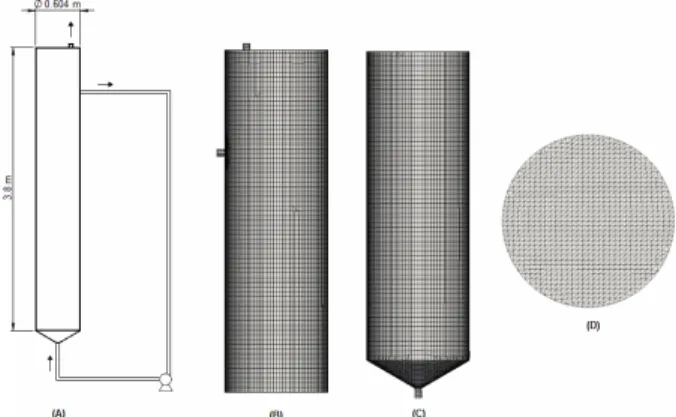
Three-dimensional meshes with different refine-ment were elaborated, in order to verify the optimal mesh to carry out the multiphase simulations. Results were obtained for meshes with refinement ranging from 60.000 to 210.000 control volumes. Comparing pressure and radial profiles of liquid velocity, it was determined in a previous work (Maurina et al., 2013) that a mesh containing approximately 130.000 vol-umes is sufficiently refined to predict accurately the behavior inside the reactor. It has y+ values (dimen-sionless measure of the thickness of the control vol-umes adjacent to the walls of the reactor) close to 37, which is suitable for turbulent case simulations. De-tails of the mesh are shown in Figures 1B, 1C and 1D.

Figure 1: (A) Schematic diagram of the bioreactor; details of the mesh used: (B) superior section, (C) in-ferior section, and (D) transversal cut.

Operating Conditions

The fluid adopted for simulations was considered to be Newtonian, with rheological properties similar to the mixture of microbial culture and substrate composed of vinasse and glycerin, discarded respec-tively in alcohol plants and biodiesel units. The gas phase has the properties of biogas, and it is initially present at the top section of the reactor. The bubble diameter was set to 0.001 m (Ding et al., 2010) with the assumption of spherical bubbles. As no reaction was considered in the simulations, biogas was as-sumed to enter at the entire base of the bioreactor, in order to consider the interaction between bubbles and the liquid phase. An approximate production of 9.259×10-5 m3/s of biogas was applied as a uniform inlet condition. A liquid flow rate of 2.25×10-3 m3/s is specified at the recirculation pipe. The outlets of liquid and gas are located in the top region. Table 2

shows the boundary conditions and physical proper-ties used in the cases proposed.

Table 2:Boundary conditions and physical

proper-ties used in the numerical simulations.

Boundary Conditions

Mixture flow rate: 2.25×10-3 m3/s

Liquid inlet

Turbulence intensity: 5%

Gas inlet Gas flow rate: 9.259×10-5 m3/s

Top outlet 101.325 Pa

Lateral outlet Fixed velocity (recirculation pipe)

Walls Smooth surface, non-slipping condition for both phases

Physical Properties

Phase Density Kinematic viscosity

Disperse (gas) 0.089 kg/m3 8.4×10-6 m2/s

Continuous

(liquid) 1.009.7 kg/m 3

1×10-6 m2/s

Bubble diameter 0.001 m

Surface tension 0.072 N/m2

Although most of the gas exits through the top outlet, a small fraction can also flow through the recir-culation pipe. Thus, the amount of liquid that leaves the reactor varies. In order to maintain the volume of liquid inside the reactor constant, an expression was elaborated to determine the liquid flow through the outlet, and use it as an inlet condition. The exact expression coded in OpenFOAM, which depends on the gas volume fraction (α_g), liquid velocity (U_l) and

the boundaries area (A), is presented in Equation (28):

(

)

, ,

,

,

1 1 l out out g out g in

l in in

U A

U A

−

= − α

α (28)

Numerical Solution

The results were obtained through simulations con-ducted with the OpenFOAM CFD toolbox, using a modified “twoPhaseEulerFoam” code. The Schiller and Naumann correlation was provided by the origi-nal code, as well as the choice to use constant values for C_L and C_VM. Other correlations evaluated in this work were included in the source code.

Brazilian Journal of Chemical Engineering FOAM, 2013). The solution of the resulting

equa-tions is made with the segregated technique, solving each set of algebraic equations separately within an iterative cycle until convergence is achieved. Nu-merical solution of the pressure-velocity coupling was performed using a mix between the SIMPLE and PISO algorithms. It involves a momentum predictor and a correction loop in which a pressure equation based on the volumetric continuity equation is solved, and the momentum is corrected based on the pressure change (Rushe, 2002).

A maximal tolerance of 10-5 for the residuals was specified to establish the convergence of the iterative solution procedure. A Courant-Friedrichs-Lewy (CFL) condition of less than 1 was applied to ensure the sta-bility of the transient solution.

t

CFL U

x

Δ =

Δ (29)

where U is the mixture velocity, Δt is the time step and Δx is the control volume size.

A total of fourteen cases were simulated to evalu-ate the influence of the interfacial forces. Five simu-lations were carried out considering only the pres-ence of the drag force, evaluated using different cor-relations. The remaining simulations considered the Zhang and Vanderheyden correlation for the drag force. Four simulations were calculated, including different correlations to estimate the lift force. One simulation considered the drag and the virtual mass forces, and another considered the three forces. The last four simulations considered the drag, drag and lift, drag and virtual mass, and all three forces, in the case of both gas and liquid phases entering the reac-tor through the recirculation pipe. Each case was cal-culated using four processes in parallel to simulate 300 s of flow, with the last 100 s used to obtain aver-age values.

RESULTS AND DISCUSSION

Drag Correlations

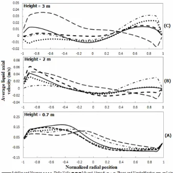
Five correlations were used to estimate the coeffi-cient of the drag force between the liquid mixture and spherical bubbles: Schiller and Naumann, Dalla Valle, Ma and Ahmadi, Zhang and Vanderheyden, and Laín. Average axial velocity profiles of the liquid phase, collected at different heights, are presented in Figure 2. Small differences can be seen in the flow pattern obtained using different drag correlations.

At the height of 0.7 m (Figure 2A), all velocity pro-files obtained presented a similar profile, with higher values between the center and the left side of the bioreactor. The velocity in this region is strongly in-fluenced by the inlet stream.

Velocity profiles observed at the height of 2 m (Figure 2B) present maximum values near the walls of the reactor. However, these values are very small, compared to those collected at the height of 0.7 m. Lower velocities can also be observed in the top re-gion of the reactor, at the height of 3 m (Figure 2C). At this position, most correlations resulted in a similar behavior, with higher velocity in the side opposite to the outlet of the reactor. Results obtained using the Schiller and Naumann correlation deviates from this behavior, showing an almost symmetrical axial velocity profile. The use of the Lain correlation resulted in a different flow pattern, with higher ve-locity on the same side of the reactor outlet. It must be emphasized that these results represent the aver-age values calculated between 200 and 300 s of flow. The mixture inside the reactor can be evaluated through its turbulent kinetic energy. Higher values of the turbulent kinetic energy indicate the presence of sub-grid vortices, which promote mixing. Thus, a weighted average of the turbulent kinetic energy (k ) was calculated, weighted by the liquid volume (Vl)

(Equation (30)).

(

)

( )

∑

∑

=

l l l

V V k k

_

(30)

With the calculation of k for each simulation, it was possible to compare how turbulent the flow is in the reactor, when simulated with different models. Another method used to compare the simulations consisted in estimating the difference of the turbulent kinetic energy (Δk) predicted in each simulation, using as reference the results obtained with the Zhang and Vanderheyden correlation (k_{l ref,} ). It is found in

the literature that this correlation gives good results in simulations of bubbles dispersed in liquid (Pang and Wei, 2011; Tabib et al., 2008). Thus, the differ-ence in the turbuldiffer-ence field predicted using other drag correlations was calculated using Equation (31).

(

)

( )

__ _{l l ref, l}

l

k k V

k

V

−

Δ =

∑

∑

Values of Δk provide a measure of the difference in the turbulent kinetic energy pattern from different simulations. Higher values indicates that the distribu-tion of the turbulent kinetic energy of two simula-tions do not agree with each other. Table 3 summa-rizes the properties defined in Equations (30) and (31).

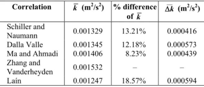
Table 3: Turbulence properties using different drag correlations.

Correlation k (m2/s2) % difference of k

__

k Δ (m2/s2)

Schiller and

Naumann 0.001329 13.21% 0.000416 Dalla Valle 0.001345 12.18% 0.000573 Ma and Ahmadi 0.001406 8.23% 0.000439 Zhang and

Vanderheyden 0.001532 – –

Laín 0.001247 18.57% 0.000594

Comparing the results, significant deviations can be seen in the weighted average turbulent kinetic en-ergy (k ), when considering different correlations for the drag force coefficient. It was found that the Laín correlation provided the lowest estimate for turbu-lence in the reactor. The analysis of Δk also con-firms that the turbulent kinetic energy field predicted using the Laín correlation was very different from the field obtained using the Zhang and Vanderheyden correlation. One explanation for this difference could be due to values of C_D tending to 16 / Re_b when using

the Laín correlation in the Stokes region, Re_b<1 (Pang and Wei, 2011). C_D values obtained using the Zhang and Vanderheyden correlation tend to 24 / Re_b in this region. It is noteworthy that the flow in the simulated bioreactor has values of Re_b around 106.20, although lower values can be found close to the walls.

Slight differences were also found using other correlations. Nonetheless, the values in Table 3 con-firm the behavior found in Figure 2, as results for tur-bulence using the Ma and Ahmadi correlation were in good agreement with results obtained using the Zhang and Vanderheyden correlation. This model also tends to 24 / Re_b in the Stokes region. Thus, it can be concluded that using different drag correlations, the predicted mean turbulence can vary as much as 18.57%, influencing the design of bioreactors.

Lift Correlations

To evaluate the effect of different lift force coeffi-cient values, four models were considered: a constant value (CL=0.5), and the correlations from Saffman, Legendre and Magnaudet, and Tomiyama. The Zhang and Vanderheyden correlation was maintained to es-timate the drag force in these cases.

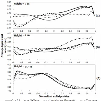
The average axial velocity profiles for the liquid phase, collected along the diameter of the reactor at the heights of 0.7 m, 2 m and 3 m, are presented in Figures 3A, 3B and 3C respectively. At the height of 0.7 m the fluid is near the inlet region; thus it is expected to have the higher velocity gradients, which interfere in the lift force calculation. It can be seen in Figure 3A that all correlations to estimate the lift force provided similar profiles for the average axial veloc-ity. Small differences were observed near the left side of the reactor, when using the Saffman correlation.

Brazilian Journal of Chemical Engineering A method used to compare the results was to

cal-culate the turbulence properties. Table 4 summarizes the results found considering different estimates for the lift force. The Legendre and Magnaudet correla-tion provides a strong dependence on both Reynolds number and the shear rate only for low Reynolds number (Hibiki and Ishii, 2007). This correlation was used to calculate the difference between the results.

Figure 3: Time-averaged axial velocity profiles of the liquid phase using different lift correlations, at the heights of (A) 0.7 m, (B) 2 m, and (C) 3 m.

Table 4:Turbulence properties using different lift correlations.

Correlation k (m2/s2) % difference of k

__

k Δ (m2/s2)

Constant C_{L 0.001376 9.03% 0.000234} Saffman 0.001341 6.30% 0.000411 Legendre and

Magnaudet 0.001262 – –

Tomiyama 0.001354 7.29% 0.000206 In Table 4, it can be noted that the use of a con-stant C_L resulted in the largest difference (9.03%), which may be due to its consideration of a high Rey-nolds number in the reactor. The Saffman correlation has a dependency on the shear rate, independent of the Reynolds number of the flow. It resulted in the higher difference of the turbulent kinetic energy field (Δk). The weighted average turbulent kinetic energy obtained with this correlation was 6.30% higher than the value obtained using the correlation from

Legen-dre and Magnaudet. The Tomiyama correlation pro-vides a dependency of C_L on Re_b at low Reynolds numbers, and it tends to a constant value of C_L=0.3 at high Reynolds numbers.

Thus, in this evaluation, it was found that dif-ferent correlations for the lift force coefficient can result in a difference of 9.03% in the estimate of the weighted average turbulence in the simulated bio-reactor.

Drag, Lift and Virtual Mass Forces

It was demonstrated that the predicted mixture in the bioreactor can be biased due to the use of differ-ent correlations to estimate the drag and lift forces. The resulting mixture can also be influenced by an inaccurate choice of forces to represent the physical phenomena.

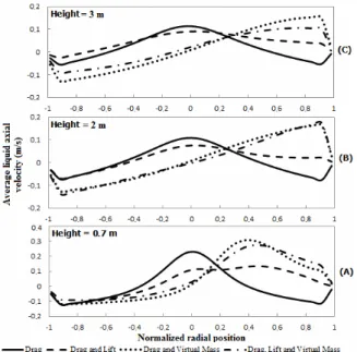
Simulations considering the drag force only (us-ing the Zhang and Vanderheyden correlation), the drag and lift forces (including the Legendre and Magnaudet correlation), the drag and virtual mass forces (con-sidering a constant coefficient C_VM =0.5), and the three forces were compared. In Figure 4, profiles for the average liquid axial velocity along the diameter of the reactor are presented, at the heights of 0.7 m, 2 m and 3 m.

Near the bottom section of the reactor, at the height of 0.7 m (Figure 4A), the liquid axial velocity profile obtained considering the drag and virtual mass forces was unlike those obtained using other models. Pro-files obtained considering all forces, the drag and lift forces, and the drag force only, agreed well among them. This indicates that, when using the virtual mass force, the lift force should also be considered, in order to have coherent results. Without these two forces, the drag force can still provide velocity pro-files in good agreement with results obtained using a more complete modeling.

At the height of 2 m (Figure 4B), the average liquid axial velocity profile obtained applying the three forces shows a maximum value on the same side of the reactor outlet. Profiles obtained using the drag and lift forces, and using the drag and virtual mass forces present an inverse behavior, with negative values in this region. On the other side, the simulation using all forces predicted an almost null liquid axial velocity, but all other cases resulted in higher values, with the highest obtained using the drag and virtual mass interfacial forces.

values at the left side of the reactor, where other simulations resulted in negative values.

The choice of interfacial forces can influence the turbulent kinetic energy, as can be seen in Table 5.

Figure 4: Time-averaged axial velocity profiles of the liquid phase considering different forces, at the heights of (A) 0.7 m, (B) 2 m, and (C) 3 m.

Table 5: Turbulence properties using different in-terfacial forces.

Force k (m2/s2) % difference of k

__

k Δ (m2/s2)

Drag 0.001531 8.38% 0.000446

Drag and lift 0.001262 10.71% 0.000484 Drag and virtual

mass 0.001479 4.64% 0.000967 Drag, lift and

virtual mass 0.001413 – –

The simulation considering the drag and lift forces resulted in the lowest weighted average turbulent ki-netic energy (k ) and, compared to the results ob-tained with the three forces, it resulted in the highest difference, 10.71%. Considering the drag and virtual mass forces, k had the lowest difference, 4.64%, but also resulted in the most different distribution of the turbulence (Δk), which is in accordance with the fields observed in Figure 4. Inaccurate prediction of the mixture can lead to bioreactors that are not optimally designed. Nevertheless, comparing these values to those obtained in the previous sections, it was found that higher differences can be obtained using different correlations for each interfacial force.

Drag, Lift and Virtual Mass Forces – One Inlet

The next four cases were carried out to analyze the consideration of different forces (drag force only, drag and lift forces, drag and virtual mass forces, and all three forces), when both gas and liquid phases are fed in only one inlet. Thus, the magnitude of each interfacial force is intensified, as well as differences among simulations.

It can be noted at the height of 0.7 m (Figure 5A) that the liquid average axial velocity profiles ob-tained disregarding the virtual mass force deviate from the results obtained by applying this force. Near the outlet (Figure 5C), these profiles are close to each other, though the profile predicted using the drag force only and using the drag and lift forces shows maximum values near the center, different from the other cases. This confirms the influence, in this case, of the virtual mass force over the flow pattern. Figure 5 also shows that the lift force, estimated with the Legendre and Magnaudet correlation, has its ma-jor influence at the bottom of the reactor, near the inlet, where high velocity gradients are present.

Figure 5: Time-averaged axial velocity profiles of the liquid phase considering different forces and one inlet, at the heights of (A) 0.7 m, (B) 2 m, and (C) 3 m.

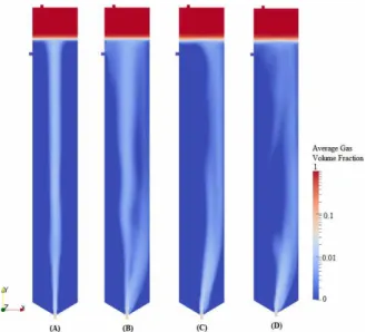
Brazilian Journal of Chemical Engineering Results obtained for the average gas volume

fraction considering the drag force only, including the lift force, the virtual mass force, and considering the three forces, are presented in Figures 6A, 6B, 6C and 6D, respectively.

The flow obtained with the drag force only is pre-sented in Figure 6A. It can be seen that bubbles are concentrated on the axis of the reactor. At higher heights, the bubble plume predicted using the Zhang and Vanderheyden correlation maintains the same behavior.

The inclusion of the lift force alters this behavior. Although the higher concentration of bubbles is still found near the center of the reactor, the plume is dispersed towards the walls. It is in accordance with the formulation of the lift force, which is transversal to the flow. Comparing Figure 6B with the average velocity profiles in Figure 5, it can be seen that the lift force is acting towards regions with higher veloc-ity – thus, with lower pressure.

In Figure 6C, the effect of virtual mass on gas distribution can be seen: the gas plume formed at the bottom of the reactor flows upward near one side of the reactor, in the region with higher velocity pre-sented in Figure 5.

The gas volume fraction field obtained with the inclusion of the three forces, illustrated in Figure 6D, shows a flow pattern similar to the field observed in Figure 6C, in which the gas plume is close to one side of the bioreactor. Moreover, the gas plume tends to disperse, as seen in Figure 6B. Thus, both the lift and virtual mass forces contribute to determine the flow pattern in the bioreactor.

The fields presented in Figure 6 are very different from those obtained considering a uniform gas inlet. In previous cases, the gas volume fraction was spread out, and most of the reactor had a small concentra-tion of disperse bubbles, without a clear difference among the cases.

As already seen in Table 5, the choice of interfa-cial forces affects the turbulent kinetic energy. Table 6 present values calculated for the simulations with gas and liquid phases fed through only one inlet. The use of only the drag force resulted in a weighted average turbulent kinetic energy (k ) close to the value obtained by applying the three forces, with a difference of only 2.72%, but also caused the most different turbulence distribution (measured with Δk). The inclusion of the lift force resulted in an average turbulent kinetic energy 4.98% lower. The inclusion of the virtual mass force increased it by 8.77%, and also resulted in a less different distribution of the turbulence (Δk). It can be seen in Figure 6 that, in spite of the close values predicted for k when considering all forces and only the drag

force, the bubble movements in these two simula-tions do not agree (Figures 6A and 6D). This empha-sizes the need to analyze the difference of the fields (Δk): its calculation shows that the use of only the drag force results in the most different turbulent kinetic energy field.

Figure 6: Time-averaged gas volume fraction, con-sidering (A) drag force only, (B) drag and lift, (C) drag and virtual mass, (D) drag, lift and virtual mass forces.

Table 6: Turbulence properties using different in-terfacial forces and one inlet.

Force k (m2/s2) % difference of k

__

k Δ (m2/s2)

Drag 0.005109 2.72% 0.001566

Drag and lift 0.004726 4.98% 0.001016 Drag and virtual

mass 0.005409 8.77% 0.000747

Drag, lift and

virtual mass 0.004973 – – Inaccurate prediction of the mixture can lead to bioreactors that are not optimally designed. Compar-ing these values to those obtained in the previous sections, it can be noted that higher differences were obtained using different correlations for each force.

CONCLUSIONS

The influence of different correlations for the drag, lift and virtual mass forces on the mixture prediction of an ASBR was verified in this paper, using the calculated turbulent kinetic energy to compare each modeling. This is an important parameter, which can be used as a measure of the mixture in the bioreactor, and thus influencing the design of new reactors.

on the liquid average axial velocity profiles under the operating conditions evaluated in this work, except for the Laín correlation. However, they affected the predicted turbulent kinetic energy, with the highest difference of 18.57%. Considering different correla-tions for the lift force coefficient, it was verified that the lift force is most meaningful near the inlet, in the bottom region of the reactor, where strong velocity gradients are expected.

The choice of forces can also lead to differences in the turbulent kinetic energy. The largest difference in the turbulent kinetic energy resulted when omit-ting the virtual mass force (10.71%), which empha-sizes the importance of this force under the operating conditions studied in this work. When considering only one inlet for both phases, the omission of the lift force resulted in a difference of 8.77%. Consider-ing only the drag force resulted in the most different turbulent kinetic energy field, measured with Δk. In cases with one inlet, and thus higher gas-liquid inter-actions, remarkable differences in the pattern of the gas volume fraction were obtained for each model.

Differences found disregarding some forces were below the differences found considering different correlations for the drag force coefficient. Thus, it is advised to carefully select the correlation to estimate each interfacial force, since they can greatly interfere with the results obtained. Provided each force are adequately estimated, the use of a more complete modeling to simulate the operational conditions found in the studied bioreactor is the safest approach to ob-tain accurate results, due to the differences found neglecting the lift and/or the virtual mass force. When possible, the model chosen must be validated with experimental values.

ACKNOWLEDGEMENTS

The authors are grateful to Petrobras and FAPERGS for their financial support.

NOMENCLATURE

Latin Letters

A boundary area (m²)

Cμ, C1, C2

constant of the k-ε turbulence model (0.09, 1.44, 1.92)

CD drag force coefficient (-) CL lift force coefficient (-)

CVM virtual mass force coefficient (-)

d diameter (m)

Eo Eötvös number (-)

g acceleration due to gravity (m s-2) I unit tensor (-)

k turbulent kinetic energy (m2 s-2) M

interphase momentum exchange term (N m-3)

MD

drag force contribution to the momentum equation (N m-3)

ML

lift force contribution to the momentum equation (N m-3)

MO

other forces contribution to the momentum equation (N m-3) MVM

virtual mass force contribution to the momentum equation (N m-3)

p pressure (Pa)

Pk

production of turbulent kinetic energy (Pa s-1)

R

combined Reynolds (turbulent) and viscous stress (m s-1)

Re Reynolds number (-) Sr dimensionless shear rate (-)

t Time (s)

U average velocity (m s-1) Ur average relative velocity (m s-1)

V volume (m³)

w

magnitude of the velocity gradient (m s-1)

Greek Letters

α volume fraction (-)

Δx control volume characteristic size (m)

ρ density (kg m-3)

υ kinematic viscosity (m2 s-1)

ε turbulent dissipation energy (m2 s-3)

σ surface tension coefficient (N m-2)

σκ, σε constant of the k-ε turbulence model

(1.0, 0.76923)

υl laminar viscosity (m2 s-1)

υt

eddy viscosity (m2 s-1)

Subscripts

b bubble eff effective

g gas phase

i phase

l liquid phase

T transposed vector

REFERENCES

Brazilian Journal of Chemical Engineering culture condition for enhanced hydrogen

produc-tion by Thermoanaerobacterium thermosaccharo-lyticum W16. Bioresource Technology, 101, p. 2053-2058 (2010).

DallaValle, J. M., Micromeritics: The Technology of Fine Particles. Pitman Publishing Co., New York (1948).

Dijkhuizen, W., van Sint Annaland, M., Kuipers, J. A. M., Numerical and experimental investigation of the lift force on single bubbles. Chemical Engineering Science, 65, p. 1274-1287 (2010). Ding, J., Wang, X., Zhou, X. F., Ren, N. Q., Guo, W.

Q., CFD optimization of continuous stirred-tank (CSTR) reactor for biohydrogen production. Bio-resource Technology, 101, p. 7005-7013 (2010). Hibiki, T., Ishii, M., Lift force in bubbly flow

sys-tems. Chemical Engineering Science, 62, p. 6457-6474 (2007).

Kantarci, N., Borak, F., Ulgen, K. O., Bubble column review. Process Biochemistry, 40, p. 2263-2283 (2005).

Laborde-Boutet, C., Larachi, F., Dromard, N., Delsart, O., Schweich, D., CFD simulation of bubble column flows: Investigations on turbu-lence models in RANS approach. Chemical En-gineering Science, 64, p. 4399-4413 (2009). Laín, S., Bröder, D., Sommerfeld, M., Goz, M. F.,

Modelling hydrodynamics and turbulence in a bubble column using the Euler-Lagrange proce-dure. International Journal of Multiphase Flow, 28 (8), p. 1381-1407 (2002).

Legendre, D., Magnaudet, J., The lift force on a spherical bubble in a viscous linear shear flow. Journal of Fluid Mechanics, 368, p. 81-126 (1998). Ma, D., Ahmadi, G., A thermodynamical formulation for dispersed multiphase turbulent flows – II: Simple shear flows for dense mixtures. Interna-tional Journal of Multiphase Flow, 16(2), p. 341-351 (1990).

Maurina, G. Z., Rosa, L. M., Beal, L. L., Baldasso, C., Pederiva, L., Torres, A. P., Optimization of a hy-drogen production bioreactor using computational fluid dynamic (CFD) techniques. Proceedings of the 13th World Congress on Anaerobic Digestion, Santiago de Compostela, Spain (2013).

Michelan, R., Zimmer, T. R., Rodrigues, J. A. D., Ratusznei, S. M., Moraes, D., Zaiat, M., Foresti, E., Effect of impeller type and mechanical agitation on the mass transfer and power consumption as-pects of ASBR operation treating synthetic waste-water. Journal of Environmental Management, 90, p. 1357-1364 (2009).

Nurtono, T., Nirwana, W. O. C., Anwar, N., Kusdianto, Nia, S. M., Widjaja, A., Winardi, S., A computa-tional fluid dynamics (CFD) study into a

hydro-dynamic factor that affects a bio-hydrogen pro-duction process in a stirred tank reactor. Procedia Engineering, 50, p. 232-245 (2012).

OpenFOAM, OpenFOAM User Guide (2013). Pang, M., Wei, J., Yu, B., Numerical study of bubbly

upflows in a vertical channel using the Euler-Lagrange two-way model. Chemical Engineering Science, 65, p. 6215-6228 (2010).

Pang, M., Wei, J. J., Analysis of drag and lift coeffi-cient expressions of bubbly flow system for low to medium Reynolds number. Nuclear Engineer-ing and Design, 241, p. 2204-2213 (2011). Pinheiro, D. M., Ratusznei, S. M., Rodrigues, J. A.

D., Zaiat, M., Foresti, E., Fluidized ASBR treat-ing synthetic wastewater: Effect of recirculation velocity. Chemical Engineering and Processing, 47, p. 184-191 (2008).

Rusche, H., Computational fluid dynamics of dis-persed two-phase flows at high phase fraction. Ph.D. Thesis, Department of Mechanical Engi-neering, Imperial College of Science, Technology and Medicine, University of London, London, UK (2002).

Saffman, P. G., The lift on a small sphere in a slow shear flow. Journal of Fluid Mechanics, 22, p. 385-400 (1965).

Schiller, L., Nauman, A. Z., A drag coefficient corre-lation. V.D.I. Zeitung, 77, p. 318-320 (1935). Tabib, M. V., Roy, S. A., Joshi, J. B., CFD simulation

of bubble column - An analysis of interphase forces and turbulence models. Chemical Engineering Journal, 139, p. 589-614 (2008).

Tomiyama, A., Tamai, H., Zun, I., Hosokawa, S., Transverse migration of single bubbles in simple shear flows. Chemical Engineering Science, 57 (11), p. 1849-1858 (2002).

Wang, X., Ding, J., Guo, W. Q., Ren N. Q., Scale-up and optimization of biohydrogen production reactor from laboratory-scale to industrial-scale on the basis of computational fluid dynamics simulation. International Journal of Hydrogen Energy, 35, p. 10960-10966 (2010).

Wang, X., Ding, J., Ren, N. Q., Liu, B. F., Guo, W. Q., CFD simulation of an expanded granular sludge bed (EGSB) reactor for biohydrogen production. International Journal of Hydrogen Energy, 34, p. 9686-0695 (2009).

Weller, H. G., Derivation, modeling and solution of the conditionally averaged two-phase flow equa-tions. Technical Report TR/HGW/02, Nabla Ltd. (2002).