http://dx.doi.org/10.1590/0103-6513.113112
Received: Dec. 4, 2012; Accepted: Apr. 21, 2014
Steady-state behavior of nonparametric control
charts using sign statistic
Shashikant Kuber Khilarea*, Digambar Tukaram Shirkeb
a*Raobahadur Narayanrao Borawake College, Shrirampur, India, [email protected] bShivaji University, Kolhapur, India
Abstract
If process is running for a long period in an in-control condition, it will reach in a steady-state condition. In order to study the long term properties of a control chart, it is appropriate to investigate the steady-state average time to signal. In this article, we discussed runs rules representation of a nonparametric synthetic control chart using sign statistic for detecting shifts in location parameter. We compared zero-state average time to signal with steady-state average time to signal of the synthetic control chart for symmetric and asymmetric distributions. We also present the m-of-m control chart using sign statistic. For comparison study, we computed average time to signal of the m-of-m control chart, the sign chart (1-of-1 chart) and the synthetic control chart for normal, Cauchy, double exponential and gamma distributions. Steady-state and zero-state performance of the m-of-m control chart with m = 2, 3 compared with the sign chart (1-of-1 chart) and synthetic control chart. The zero-state and steady-state average time to signal of the synthetic and the m-of-m control charts computed using Markov chain approach.
Keywords
Steady-state. Markov chain. Synthetic. Nonparametric. Average time to signal.
1. Introduction
In a process control environment with variables data, it is assumed that the process output follow the normal distribution. The statistical properties of commonly employed control charts such as the Shewhart X chart, the cumulative sum control chart and the exponentially weighted moving average control chart are the exact only if assumption of normality is satisfied. If the underlying process distribution is non-normal, performance of these charts are not up to the mark. Such considerations provide reasons for the development and applications of control charts that are not specifically designed under the assumption of normality or any other parametric distribution. When the distribution of process output is non-normal, distribution-free or nonparametric control charts can be useful.
Nonparametric control charts are used for detecting the changes in the process median (or mean) or changes in the process variability. Most of the control charts are based on the sample means when observations
a higher probability than for normal distribution. In nonparametric control charts variance of the process need not to be known or estimated in order to apply the control chart. In fact, these control charts for controlling median are not affected by changes in the variance as long as location parameter is constant. The nonparametric control charts may be particularly useful when a process is just start up. It is desirable to apply control charts before there is an enough data to get a reasonable estimate of variance and/ or assess the normality of the process.
In quality control applications McGilchrist
& Woodyer (1975) proposed a distribution-free cumulative sum technique for monitoring rainfall amounts. Bakir (2006) developed distribution-free quality control charts based on signed-rank-like statistic. Bakir (2004) proposed a distribution-free Shewhart quality control chart based on signed-ranks. Bakir & Reynolds Junior (1979) studied a nonparametric procedure for process control based on within-group ranking. Amin & Searcy (1991) studied the behavior of the EWMA control chart using the Wilcoxon signed-rank statistic. Amin et al. (1995) developed the nonparametric quality control charts based on the sign statistic. Chakraborti & Eryilmaz (2007) proposed control charts based on signed-rank statistic. Chakraborti & Van de Wiel (2008) proposed Mann-Whiteny statistic based control chart. Human et al. (2010) studied nonparametric Shewhart-type sign control charts based on runs. Ho
& Costa (2011) proposed monitoring a wandering mean with an np chart and this chart is also work with sign statistics. Crosier (1986) suggested a technique for obtaining steady-state ARL of CUSUM chart using the Markov chain approach. Saccucci & Lucas (1990) given a FORTRAN computer program for the computation of ARL of EWMA and combined Shewhart-EWMA control schemes. The program calculates zero-state and steady-state ARL using the Markov chain approach. Champ (1992) computed steady-state ARL of Shewhart control chart with supplementary runs rules. Davis & Woodall (2002) studied the steady-state properties of synthetic control chart to monitor shifts in process mean. Lim & Cho (2009) developed a control charts with m-of-m runs rules to study the economical-statistical properties of control chart using steady-state ARL.
The rest of article is organized as follows: Section 2 gives the Shewhart charts using sign statistic. Section 3 gives conforming run length control chart. In Section 4, operations and design procedure of synthetic control chart using sign statistic are given and also in this we explained the Markov chain model and steady-state ATS of synthetic control chart. In Section 5, we present m-of-m runs rules
schemes using sign statistic. In this Section, we also study steady-state and zero-state ATS performance of the m-of-m chart for process median. Section 6 gives conclusions.
The Shewhart control chart using sign statistic is explained in brief in following section.
2. Shewhart chart using sign statistic
Let X be a continuous random variable with cumulative distribution function (c.d.f.) F(.). Let
m and m0 be the median and target value of median respectively. A sample of n observations is taken at regular time interval from the process. Let Xi = (Xi1,Xi2,...,Xin) be the sample taken at the ith time point. At any time t, each observation from the sample is compared with target value m0 and the number of observations above and below m0 is recorded.
Define,
0
0 0
0
1
( ) 0
1
ij
ij ij
ij
if X
sign X if X
if X
m
m m
m >
− = = − <
(1)
where Xij is the jth observation in the ith sample. Since the distribution of observations is assumed to be continuous, pr(Xij – m0 = 0) = 0. In practice occasional zero may occur which can be signed alternatively +1 and -1.
Let
0 1
( ) 1, 2,3,...
n
i ij
j
SN sign X m i
=
= − =
∑
(2)where SNi is the difference between number of observations above m0 and number of observations below
m0 in the ith sample. A random variable T
i = SNi + n/2 gives the number of positive signs in the sample of size n and has binomial distribution with parameters n and p, where p = P(Xij > m0). As long as median remains at m0, we have p = p0 = 1/2. That is, P(Xij > m0) = P(Xij < m0) = 1/2 and E[SNi] = 0. The chart signals that shift has occurred if |SNi| ≥ c, where c >0 is a specified constant (upper control limit = c and lower control limit = -c). The chart signals that shift has occurred in the positive direction if SNi≥ c and chart signals that the shift has occurred in the negative direction if SNi< –c.
The largest possible in-control average run length (ARL) values of symmetric one-sided and two-sided control chart are 2n and 2n-1 respectively, when p = 1/2 and SNi = n. Unless ‘n’ is of a moderate size, it may be difficult to achieve even approximately a specified in-control ARL (0).
nonconforming shift and be equal to the product of mCRL and ARLCRL.
1 1
1 (1 )
CRL CRL CRL
CRL L
ANI ARL
ANI
p p
m = × = ×
− − (7)
For CRL chart, if a CRL value falls between lower and upper control limits of the CRL chart, then the process is considered to be under control. However, if CRL value is less than the lower control limit of CRL chart, then upward process shift is signaled and if CRL value greater than upper control limit of CRL chart, then downward process shift is signaled. The presentation of CRL chart usually based on the 100% inspection, because every unit has to be accounted for and classified as either conforming unit or nonconforming one.
In following section we explain synthetic control chart using sign statistic.
4. Synthetic control chart using sign
statistic
In the literature, Wu&Spedding (2000) studied the synthetic control chart for detecting small shifts in the process mean. Wu et al. (2001) proposed the synthetic control chart for fraction nonconforming and reported that the synthetic control chart has higher power of detecting out-of-control signal. Wu
&Spedding (2001) developed the synthetic control charts for attributes. Khilare & Shirke (2010) proposed a nonparametric synthetic control chart using sign statistic and it performs significantly better than the Shewhart type X and sign control charts. The proposed nonparametric synthetic control chart is a combination of the nonparametric sign chart and the CRL chart. Basically, the operations of the nonparametric synthetic control chart are similar to that of the synthetic control chart for process mean proposed by Wu&Spedding (2000), except that the
3. The conforming run length control
chart
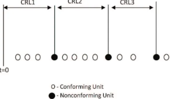
The conforming run length (CRL) chart is proposed by Bourke (1991). The Conforming run length is the number of inspected units between two consecutive nonconforming units including ending nonconforming unit. In Figure 1 below, the white and black circles denote the conforming and nonconforming units respectively. Suppose process start at t=0, then the three samples of CRL are displayed. CRL1=4, CRL2=5, CRL3=3. The idea behind the CRL chart is that the conforming run length will change when the fraction nonconforming in a process p changes. Namely, the CRL is shortened as p increases and is lengthened as p decreases (Figure 1).
The random variable CRL follows a geometric distribution. The probability mass function of CRL is
( ) (1 )CRL, 1, 2,3,...
P CRL =p −p CRL= (3)
The cumulative probability function and mean value of CRL are respectively
( ) 1 (1 )
1
CRL
CRL
F CRL p
p
m
= − − =
(4)
If CRL is less than lower control limit (L) of CRL chart, then an upward process shift is signaled. Therefore, for detection of an upward process shift (increase in p), a single lower control limit L of CRL chart is sufficient and L can be derived from Equation 4, we have,
( ) 1 (1 )
ln(1 )
ln(1 0)
L CRL
CRL
F L p
L
p
a a = = − −
− =
− (5)
where aCRL is the type-I error probability of the CRL chart and p0 is the in-control fraction nonconforming. L must be rounded to an integer. If a sample CRL is a less than or equal to the L, then the fraction nonconforming p has increased and out-of-control status will be signaled.
For the CRL chart, ARLCRL, is the average number of CRL samples required to detect out-of-control fraction nonconforming p is given by
1
1 1 (1 )
CRL CRL
CRL L
ARL
ARL
p
a =
=
− − (6)
Finally, let ANICRL be the average number of the inspected units required to signal a fraction
( )
(
1( )
)
(0)
0 [1 1 0 L]
ARLs
P P
=
− − (9)
and P(d) = Pr(SNi > c/m = m0 + d).
Here, P(d) is the probability that the sample is nonconforming when the permanent upward step shift of d units occurs. When there is no shift, d is equal to zero. We note that in Equation 7, “p” is the probability that a unit is nonconforming.
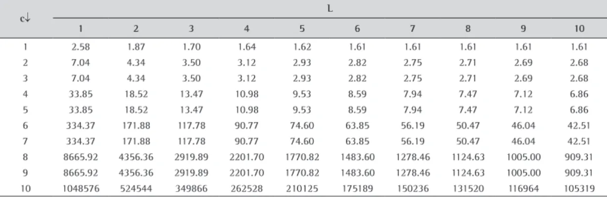
Suppose the desired in-control ARL is ARL(0) and the subgroup sample size is n. We compute the ARLs(0) values using Equation 9 for c = 1, 2, …,n and L = 1, 2, … . Now choose that pair of (L, c) for which the ARLs(0) is close to ARL(0). We may note that for a fixed value of c, ARLs(0) is a decreasing function of L, while for a fixed value of L, ARLs(0) is a non-decreasing function of c.
Table 1 gives the values of ARLs(0) for n = 10. As an example, suppose we wish to set ARL(0) = 1024. Then, from Table 1, we see that L = 9 and 8 = 10 is the required pair as the ARLs(0) corresponding to these values is 1005. Due to the discrete nature of the charting statistic SNi, for a fixed value of L, we get the same value of ARLs(0) for two successive values of c (except for c = 1).
The complete design procedure for the synthetic chart can be outlined as below:
1 Specify subsample size n and ARL(0). 2 Initialize L as 1 and 1 ≤ c ≤ n.
3 Calculate ARLs(0) from the current values of L and c using Equation 9.
4 If ARLs(0) is not close to the specified in-control ARL, increase L by one and go to step 3.
5 If ARLs(0) is close to the specified in-control ARL, take current values of L and c as final values in the synthetic control chart.
In following section we discuss runs rule representation of the synthetic control chart. subgroup mean is replaced by the sign statistic SNi.
However, we do not follow the same design procedure due to Wu&Spedding (2000) in order to ensure that the synthetic control chart is nonparametric.
The operations of the synthetic chart using sign statistic are outlined below.
1 Determine sign chart based upper control limit ‘c’ ( > 0), sample size n and CRL based lower control limit (L).
2 Take a sample of ‘n’ units for inspection and calculate SNi.
3 If SNi < c, a sample is a conforming one and control flow goes back to step (2). Otherwise, a sample is a nonconforming one and control flow continues to the next step.
4 Check number of samples between the current and previous nonconforming samples. This number is taken as CRL value for synthetic chart.
5 If CRL > L, then the process is said to be under control and control flow goes back to the step (2). Otherwise the process is taken as out-of-control and control flow continues to the next step. 6 Take action to locate and remove the assignable
causes. Then go back to step (2).
4.1.
Design of synthetic control chart
The synthetic chart has two parameters namely, L and c. For given in-control ARL and subgroup sample size n, the parameters L and c are obtained as follows:
Let ARLs(m) be the out-of-control ARL of the synthetic control chart and it is given by
( )
(
1( )
)
( )
[1 1 ]
S L
ARL
P P
m
d d
=
− − (8)
Let ARLs(m0) be in-control ARL of the synthetic control chart. If m0 = 0, then in-control ARL is
Table 1. In control ARL values for upward sided synthetic control chart for various values of c and L when n = 10.
c↓ L
1 2 3 4 5 6 7 8 9 10
1 2.58 1.87 1.70 1.64 1.62 1.61 1.61 1.61 1.61 1.61
2 7.04 4.34 3.50 3.12 2.93 2.82 2.75 2.71 2.69 2.68
3 7.04 4.34 3.50 3.12 2.93 2.82 2.75 2.71 2.69 2.68
4 33.85 18.52 13.47 10.98 9.53 8.59 7.94 7.47 7.12 6.86
5 33.85 18.52 13.47 10.98 9.53 8.59 7.94 7.47 7.12 6.86
Consider the case where L = 4. This chart is an identical to a chart which signals if two of the five consecutive sign statistics fall out-sides of the control limits, assuming that a sign statistic at time zero is out-side of control limits.
Let
A= Pr[next observed sign statistic will be within control limit/ limits]
The probability of next observed sign statistic will be within control limits for the change in location parameter is
A = Pr[–c < SNi < c],
and for shift in positive direction A = Pr[SNi≤ c],
where, ‘c’ is a specified constant (control limit of sign control chart) and B= 1- A.
As Davis & Woodall (2002) suggested that the following transition matrix would govern the Markov chain for the synthetic control chart.
• The row contains ‘A’ in first column and ‘B’ in second
column.
• The last row contains ‘A’ in first column.
• In all other rows, the entry above the diagonal is ‘A’. • In all other locations, the entry is zero.
Therefore, for example, the transition probability matrix for the synthetic control chart using sign statistic when L= 4 is (Table 2).
With this Markov chain model, the ARL for the zero-state case is
ARL = s’(I – R)–11 (10)
where, R is an L+1 by L+1 matrix of probabilities obtained by deleting last row and last column from the above matrix, 1 is column vector of appropriate order having all elements unity and I is an (L + 1) by (L + 1) identity matrix, s is the order (L + 1) of initial probabilities, 1 for initial state and 0 for the
4.2.
Runs rule representation of the
synthetic control chart
Davis & Woodall (2002) discussed the runs rule representation of synthetic control chart to detect shifts in the process mean. Here, we discuss the runs rule representation of a nonparametric synthetic control chart for process median using sign statistic. Suppose that each observed sign statistic SNi is classified as either ‘0’ (conforming) or 1 (nonconforming). If value of sign statistic falls within control limit/limits, the sample is conforming and if it falls out-side the control limit/limits then sample is nonconforming. A sequence of SNi can be represented by a string of zeros and ones. For example 10001000 would indicate that in a sequence of eight samples, the first and fifth samples are nonconforming samples.
For simplicity, suppose that L = 3. This means that any sequence of SNi with pattern 1001, 101 or 11 will generate an out-of-control signal for synthetic chart. Note that this sequence also generate signal under the following runs rule:
If two successive sign statistics (SNi values) fall out-side of the control limits out of L + 1 sign statistics then the two-of-L+1 chart signals an out-of-control status.
On initial pattern of 001, the synthetic control chart will signal using L=3, while two of L + 1 chart would not. The performance of control charts can be made identical over all the samples using head start feature in the runs rule representation; that is , it is assumed that the there is an observation at time zero and that falls out-side of the control limits. With this head start, both charts will signal on initial patterns 1, 01, and 001 but not on the initial pattern 0001. Thus, performance of the charts is now identical for all possible sequences of SNi. If CRL value is less than or equal to L, then declare that the process is out-of-control. Thus, the synthetic control chart using sign statistic is identical to the above runs rule with the head start a sign statistic at time zero is observed and is nonconforming.
In the following subsection, we present the Markov chain model and ARL results of synthetic control chart.
4.3.
The Markov chain model and
steady-state ATS of synthetic control chart
The formula for ARL can be obtained by using the transition probability matrix (t. p. m.) of an absorbing Markov chain based on the states depending on a lower control limit of the CRL chart.
Table 2. The transition probability matrix for the synthetic control chart using sign statistic when L= 4 is:
States at time t+1
↓States→ 0000 0001 0010 0100 1000 Signal
States at time t
0000 A B 0 0 0 0
0001 0 0 A 0 0 B
0010 0 0 0 A 0 B
0100 0 0 0 0 A B
1000 A 0 0 0 0 B
zero-state ATS with steady-state ATS of the synthetic control chart. For performance study of the synthetic chart, we consider symmetric distributions namely normal, Cauchy, double exponential distributions and asymmetric gamma distribution. ATS is computed for double exponential distribution, which is symmetric distribution with heavy tails. Cauchy distribution is used because it is symmetric distribution with extremely heavy tails. ATS values computed for each considered distributions with mean zero and variance one. In Bakir (2004) the scale parameter is set to be 1
2 for double exponential distribution to achieve variance equal to one. To compute SSATS of Cauchy distribution, scale parameter set to be one and shifts in location parameter. For gamma distribution parameters are set to be 4 (shape parameter ) and 1/2 ( scale parameter ) to achieve mean zero and variance one. Control limits for each control charts are found to be such that the in-control ATS equal to the desired ATS.
Table 3 gives the zero-state and steady-state ATS profile of the synthetic control chart to detect upward shifts in the process median. For the synthetic control chart sample sizes of n = 10 is used. In-control ATS for n =10 is 1024.
The following findings are observed from Table 3.
• Steady-state ATS performance of the synthetic
control chart is poor as compare to zero-state for all distributions under study.
• Steady-state performance of the synthetic control
chart for double exponential distribution is better than the other distributions under study.
Following section gives the m-of-m control chart using sign statistic for monitoring location parameter.
5. The m-of-m control chart
Consider a control chart with upper control limit (UCL= k) and lower control limit (LCL= -k). Let us consider three regions for the control chart:
• The region between upper control limit and lower
limit (region 1).
• The region above upper control limit (region 2). • The region below lower control limit (region 3).
The probability of a single point falls in the regions 1, 2, 3 are denoted by pc, pu, pl respectively and these probabilities can be computed as follows:
[
]
Pr ,
Pr ,
2 2
i
i
pc k SN k
k n k n
T
= − < < − + +
= < <
rest of the cases, s’= [0, 1, 0,…, 0, 0]. Here, ‘01’ corresponds to the initial state. For general values of L, the matrix R (the matrix of probability above with the last row and last column removed) will be an (L + 1) by (L + 1) matrix.
Since the Markov chain representation of the synthetic control chart using sign statistic has more than one absorbing states. The future behavior of the chart can be studied by using steady-state average time to signal (SSARL). If the process is running smoothly for long time, it reaches in the steady-state. The SSARL measures average number of samples required to signal when the effect of head start has disappeared.
Let R0 be the square matrix obtained from R after dividing each element by the corresponding row sum. Let S be a row vector corresponding to the stationary probability distribution of R0. The SSARL of the synthetic chart using sign statistic is given by
SSARL = S’(I –R0)–11 (11)
The S can be obtained by solving following equation
S = R’0S, subject to
1
1
n i i
S
=
=
∑
Finally steady-state average time to signal (SSATS) is given by,
( )
1 2
SSATS=SSARL− h (12)
Where, sampling interval (h) is adjusted according to the desired rate of false alarms rate. The SSATS measures the average time required to signal a process shift when the effect of head start has disappeared.
We provide steady-state performance of the synthetic control chart in the following section.
4.4.
Steady-state performance of the
synthetic control chart
only if starting from state one, the probability of returning to state one after some finite length of time is less than one. Then the 2m × 2m transition probability matrix can be partitioned as
( )
0 1
Q I Q J P= −
where, Q is the (2m – 1) × (2m – 1) transition probability matrix for the transient sates, I is the (2m – 1) × (2m – 1) identity matrix and J is the column vector of one of an order (2m – 1). The expected value of the run length random variable T is given by
[ ]
(
)
1E T =e I−Q− J (13)
where, e1×2m–1 = (1,0,0,...,0) is the initial distribution. Let Mj be the expected value of the waiting time from state j until the first occurrence of D. Thus, if process is initially in-control, M1 is the ARL. Let M = (M1,M2,...,M2m–1) be the vector of average run lengths. By taking expectations conditional upon the result of the first subgroup these expected values can be found by solving the following linear system of equations corresponding to (I – Q)J = 1, where 1 is the column vector of one’s.
1 1 2 3
2 1 3 4
3 1 2 5
4 1 3 6
5 1 2 7
2 4 1 3 2 2
2 3 1 2 2 1
2 2 1
1 . . . ,
1 . . . ,
1 . . . ,
1 . . . ,
1 . . . ,
. . .
1 . . .... . ,
1 . . ... . ,
1 .
m m
m m
m
M pc M pu M pl M
M pc M pu M pl M
M pc M pu M pl M
M pc M pu M pl M M pc M pu M pl M
M pc M pl M pu M
M pc M pu M pl M
M pc M p
− −
− −
−
= + + + = + + + = + + + = + + + = + + +
= + + + + = + + + + = + + 3
2 1 1 2
. ,
1 . . .
m
l M
M − = +pc M +pu M
[
]
[
]
2 ,
Pr ,
Pr .
i i
i i
SN T n
pu SN k
pl SN k
= − = ≥ = ≤ −
The m-of-m sign chart signals an out-of-control status when a sign statistic falls out-side of the control limits or m-consecutive sign statistics falls beyond the control limits. Suppose {mm} denotes the event when two successive sign statistics fall in region m. The control chart signals an out-of-control status when an event 222...2 ,333...3
m times m times
D
− −
=
occurs. To design
this control chart we must find appropriate control limits to keep in-control ATS at the desired level.
Now we define states of the Markov chain as follows:
State 1: One point fall between both control limits, {1}.
State 2: One point falls above upper control limit, {2}.
State 3: One point falls below lower control limit, {3}.
State 4: Two consecutive points fall above upper control limit, {22}.
State 5: Two consecutive points fall below lower control limit, {33}.
State 6: Three consecutive points fall above upper control limit, {222}.
State 7: Three consecutive pints fall below lower control limit, {333} and so on.
Finally,
State 2m: Out-of-control (absorbing) state, with associated pattern given by the set D.
The Markov chain representation of chart consist of 2m states with the first (2m – 1) of them being transient. A state is said to be transient state if and
Table 3. Zero-state and steady-state ATS profile of the synthetic chart to detect upward shifts in process median (n=10, c = 9, L = 9 and ATS(0) = 1024).
(m – m0)
Normal Distribution Cauchy Distribution Laplace Distribution Gamma Distribution
0SATS SSATS 0SATS SSATS 0SATS SSATS 0SATS SSATS
0 1024.59 1024.63 1024.59 1024.63 1024.59 1024.63 1024.01 1024.06
0.1 305.76 321.91 386.88 402.54 148.50 163.01 294.28 310.43
0.2 104.90 117.83 161.35 176.20 36.80 44.65 101.63 114.40
0.3 41.40 49.79 74.79 86.04 13.45 17.51 41.48 49.87
0.4 18.75 23.91 38.52 46.59 6.52 8.70 19.67 25.00
0.5 9.69 12.81 21.93 27.66 3.86 5.07 10.65 14.03
0.6 5.64 7.52 13.67 17.78 2.61 3.30 6.47 8.63
0.7 3.64 4.76 9.22 12.21 1.94 2.33 4.31 5.70
0.8 2.55 3.21 6.65 8.87 1.52 1.74 3.10 4.00
0.9 1.90 2.28 5.06 6.74 1.24 1.37 2.36 2.94
1 1.48 1.69 4.04 5.32 1.05 1.12 1.88 2.25
By solving the above linear system of equations, the ARL M1 for a chart with m-of-m runs rule (m > 1) is given by,
(
)(
)
( )( )
(
)(
) (
)(
)
1 1 1
1 1
1 1 . 1 1 1 1
m m
m m m m
pu pl
M
pu pl pu pl pu− pl − pc pu pl
− −
=
− − − − − − − −
The 1-of-1 chart signals an out-of-control status if a sign statistic falls either above upper control limit or below a lower control limit. The 2-of-2 chart signals an out-of-control status if two consecutive sign statistics fall either above an upper control limit or below lower control limit. In other words, if two successive sign statistics fall in the region 2 or region 3, the 2-of-2 chart signals an out-of-control status. The 3-of-3 chart signals an out-of-control status if three consecutive sign statistics fall either above upper control limit or below lower control limit.
Following subsection gives steady-state average time to signal of the m-of-m control chart.
5.1.
Steady-state average time to signal
If process is running for a long period in an in-control condition, it will reach in a steady-state condition. In order to study the long term properties of a control chart, it is appropriate to investigate the steady-state average time to signal.
Let Q0 be a square matrix obtained from Q by imposing the condition that no signal occurs. Let
pT = [p
1,p2,...,p2m–1] be the vector of steady-state probabilities for the in-control transient states. The steady-state probabilities can be obtained by solving the following equations: pTQ
0 = p
T and pT1 2m–1 = 1. Under the in-control situation p = p0, let p1 = pc and u = pc = pl.
The SSARL can be obtained by SSARL = pT ARL
and SSATS computed using Equation 12.
Steady-state performance of the m-of-m control chart is given in following subsection.
5.2.
Steady-state performance study of the
m-of-m control chart
For efficiency comparisons, we compare the proposed m-of-m chart with the synthetic, Shewhart type X and sign control charts in terms of their out-of-control steady-state ATS and zero state ATS. The results are shown in Tables 4-11 for subgroup of size 11 under normal, double exponential, Cauchy and gamma distributions.
Following are the findings from Tables 4 to 11:
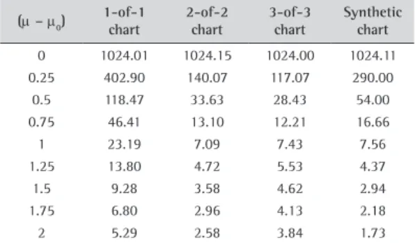
Table 4. SSATS of the m-of-m and synthetic control charts for normal distribution (n=11 and SSATS(0) =1024).
(m – m0) 1-of-1 chart
2-of-2 chart
3-of-3 chart
Synthetic chart 0 1024.01 1024.15 1024.00 1024.11 0.25 278.48 88.47 73.12 173.04 0.5 57.40 16.05 14.53 21.52
0.75 16.40 5.38 6.05 5.22
1 6.19 2.81 4.01 2.00
1.25 2.92 2.00 3.43 1.03
1.5 1.64 1.73 3.28 0.67
1.75 1.07 1.64 3.25 0.53
2 0.79 1.62 3.25 0.48
Table 5. Steady-state ATS of the m-of-m and synthetic control charts for Cauchy distribution. (n=11 and SSATS(0)=1024).
(m – m0)
1-of-1 chart
2-of-2 chart
3-of-3 chart
Synthetic chart 0 1024.01 1024.15 1024.00 1024.11 0.25 402.90 140.07 117.07 290.00 0.5 118.47 33.63 28.43 54.00 0.75 46.41 13.10 12.21 16.66
1 23.19 7.09 7.43 7.56
1.25 13.80 4.72 5.53 4.37
1.5 9.28 3.58 4.62 2.94
1.75 6.80 2.96 4.13 2.18
2 5.29 2.58 3.84 1.73
Table 6. Steady-state ATS of the m-of-m and synthetic control charts for double exponential distribution. (n=11 and SSATS(0)=1024).
(m – m0) 1-of-1 chart
2-of-2 chart
3-of-3 chart
Synthetic chart 0 1024.01 1024.15 1024.00 1024.11 0.25 115.84 32.83 27.80 52.42
0.5 22.02 6.79 7.19 7.15
0.75 7.60 3.16 4.29 2.42
1 3.66 2.18 3.55 1.25
1.25 2.17 1.83 3.34 0.82
1.5 1.47 1.70 3.27 0.63
1.75 1.11 1.64 3.25 0.54
2 0.89 1.63 3.25 0.49
Table 7. Steady-state ATS of the m-of-m and synthetic control charts for gamma distribution. (n=11 and SSATS(0)=1024).
(m – m0)
1-of-1 chart
2-of-2 chart
3-of-3 chart
Synthetic chart 0 1024.00 1024.03 1024.01 1024.00 0.25 275.40 87.15 72.03 170.04
0.5 63.25 17.52 15.69 24.01
0.75 20.98 6.41 6.88 6.61
1 9.23 3.45 4.51 2.77
1.25 5.02 2.39 3.70 1.50
1.5 3.21 1.95 3.40 0.97
1.75 2.31 1.76 3.30 0.72
Table 8. Zero-state ATS of the Shewhart type X, m-of-m and synthetic control charts for normal distribution (n=11 and SSATS(0)=1024).
(m – m0) X chart 1-of-1 chart 2-of-2 chart 3-of-3 chart Synthetic chart 0 1024.02 1024.01 1024.22 1024.41 1024.13 0.25 146.39 278.48 88.66 73.60 160.28
0.5 19.26 57.40 16.15 14.81 17.11 0.75 4.29 16.40 5.43 6.25 3.91
1 1.47 6.19 2.85 4.17 1.62
1.25 0.75 2.92 2.03 3.58 0.94 1.5 0.55 1.64 1.76 3.43 0.66 1.75 0.51 1.07 1.67 3.40 0.55
2 0.50 0.79 1.65 3.40 0.50
Table 9. Zero-state ATS of the Shewhart type X, m-of-m and synthetic control charts for Cauchy distribution (n=11 and SSATS(0)=1024).
(m – m0) X chart
1-of-1 chart
2-of-2 chart
3-of-3 chart
Synthetic chart 0 1024.05 1024.01 1024.03 1024.41 1024.13 0.25 1024.04 402.90 140.27 117.61 276.18 0.5 1024.04 118.47 33.76 28.78 46.16 0.75 1024.03 46.41 13.19 12.46 13.00 1 1024.01 23.19 7.15 7.64 5.67 1.25 1023.99 13.80 4.78 5.71 3.29 1.5 1023.97 9.28 3.63 4.79 2.27 1.75 1023.94 6.80 3.00 4.29 1.75 2 1023.90 5.29 2.62 4.00 1.44
Table 10. Zero-state ATS of the Shewhart type X, m-of-m and synthetic control charts for Laplace distribution (n=11 and SSATS(0)=1024).
(m – m0) X chart 1-of-1 chart 2-of-2 chart 3-of-3 chart Synthetic chart 0 1024.06 1024.01 1024.03 1024.41 1024.13 0.25 218.58 115.84 32.96 28.15 44.71
0.5 32.17 22.02 6.86 7.40 5.35 0.75 6.70 7.60 3.21 4.45 1.92
1 1.96 3.66 2.21 3.70 1.10
1.25 0.87 2.17 1.86 3.48 0.78 1.5 0.58 1.47 1.73 3.42 0.63 1.75 0.51 1.11 1.68 3.40 0.55
2 0.50 0.89 1.66 3.40 0.52
Table 11. Zero-state ATS of the Shewhart type X, m-of-m and synthetic control charts for gamma distribution (n=11 and SSATS(0)=1024).
(m – m0) X chart
1-of-1 chart
2-of-2 chart
3-of-3 chart
Synthetic chart 0 1024.09 1024.00 1024.19 1024.00 1024.00 0.25 249.23 275.40 87.35 72.48 157.34 0.5 38.20 63.25 17.62 15.97 19.25 0.75 12.64 20.98 6.47 7.08 4.95
1 6.19 9.23 3.50 4.68 2.16
1.25 3.79 5.02 2.43 3.85 1.28 1.5 2.66 3.21 1.98 3.55 0.89 1.75 2.06 2.31 1.79 3.45 0.70
2 1.71 1.82 1.70 3.41 0.60
• For small to moderate shifts the SSATS and 0SATS
performance of the m-of-m chart with m=2, 3 is significantly better than the Shewhart type X, sign and synthetic control charts.
• Performance of sign chart under normal distribution
and double exponential distribution is better as compare to m-of-m chart with m=2,3 only for a few large shifts.
• Synthetic control chart performs better than the sign
chart through-out shifts; however, its performance is better as compared to m-of-m chart with m=2, 3 only for large shifts under all distributions.
• The SSATS performance of the 3-of-3 control chart is
better than the 2-of-2 control chart for all distributions only for small shifts.
• The SSATS performance of all control charts under
double exponential distribution is better than the gamma, Cauchy and normal distributions to monitor process median.
• It is also observed that the SSATS values and 0SATS
values are not significantly differ.
5.3.
Numerical example
We illustrate the operations of the proposed m-of-m control chart using data generated from standard normal distribution. The data set includes 21 samples each
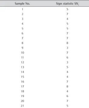
of 11 observations. We assumed that the in-control median m0 = 0. To have an in-control ARL equal to 1024, the upper control limits of 1-of-1 chart, 2-of-2 chart and 3-of-3 chart are 11, 8 and 6 respectively. The lower control limits of these control charts set to be zero. Table 11 gives the values of the sign statistic SNi for 21 samples. We have constructed 1-of-1 chart, 2-of-2 chart and the 3-of-3 chart in Figure 2. The 1-of-1 chart (sign chart) signals if a sign statistic falls above upper control limit of sign chart, the 2-of-2 chart signals if when two consecutive sign statistics fall above upper control limit of the 2-of-2 chart and when three consecutive sign statistics fall above upper control limit of the 3-of-3 chart, the 3-of-3 control chart signals (Table 12).
From Figure 2, we see that no points exceed the control limits of the 1-of-1 chart and 2-of-2 chart. Consequently, one might regard the process as being in a state of statistical control. From Figure 2 it is also observed that the points 6, 7 and 8 fall above the upper control limit of the 3-of-3 chart. Therefore, the 3-of-3 chart signal at point 8.
Table 12. Sample numbers and values of sign statistic.
Sample No. Sign statistic SNi
1 5
2 7
3 4
4 5
5 5
6 7
7 7
8 8
9 3
10 7
11 6
12 3
13 5
14 4
15 4
16 7
17 8
18 4
19 6
20 7
21 5
Figure 2. The m-of-m control chart with m = 1, 2, 3.
We have investigated the steady-state ATS of a nonparametric synthetic and the m-of-m control charts based on sign statistic. The proposed charts are used to monitor shifts in a process median. The SSATS values of proposed charts are computed by employing Markov chain approach. The steady-state performance of the m-of-m chart with m=2, 3 is significantly better than the sign chart (1-of-1 chart) and the synthetic control chart. Also, the steady-state ATS performance of the synthetic control chart is poor as compared to the zero-state ATS. The m-of-m control chart with m=2, 3 has a higher power of
detecting out-of-control signal than the sign chart and the synthetic control chart.
References
Amin, R. W., & Searcy, A. J. (1991). A nonparametric exponentially weighted moving average control schemes. Communications in Statistics: Simulation and Computation, 20(4), 1049-1072. http://dx.doi. org/10.1080/03610919108812996
Amin, R. W., Reynolds Junior, M. R., & Bakir, S. T. (1995). Nonparametric quality control charts based on the sign statistic. Communications in Statistic: Theory and Methods, 24(6), 1597-1623. http://dx.doi. org/10.1080/03610929508831574
Bakir, S. T. (2004). A distribution-free shewhart quality control chart based on signed-ranks. Quality Engineering, 16(4), 613-623. http://dx.doi.org/10.1081/ QEN-120038022
Bakir, S. T. (2006). Distribution-free quality control charts based on signed-rank-like statistic. Communications in Statistics: Theory and Methods, 35(4), 743-757. http:// dx.doi.org/10.1080/03610920500498907
Bakir, S. T., & Reynolds Junior, M. R. (1979). A nonparametric procedure for process control based on within-group ranking. Technometrics, 21(2), 175-183. http://dx.doi.or g/10.1080/00401706.1979.10489747
Bourke, P. D. (1991). Detecting a shift in fraction nonconforming using run length control chart with 100% inspection. Journal of Quality Technology, 3(2), 51-68.
Chakraborti, S., & Eryilmaz, S. (2007). A nonparametric shewhart-type signed-rank control chart based on runs. Communications in Statistic, 36(2), 335-356. http:// dx.doi.org/10.1080/03610910601158427
Chakraborti, S., & Van de Wiel, M. A. (2008). A nonparametric control charts based on mann-whitney statistic. IMS Collection, 1, 156-172. http://dx.doi. org/10.1214/193940307000000112
Statistics: Theory and Methods, 39(18), 3282-3293. http://dx.doi.org/10.1080/03610920903249576 Lim, T., & Cho, M. (2009). Design of control charts with
m-of-m runs rules. Quality and Reliability Engineering International, 25(8), 1085-1101. http://dx.doi. org/10.1002/qre.1023
McGilchrist, C. A, & Woodyer, K. D. (1975). Note on a distribution-free CUSUM technique. Technometrics, 17(3), 321-325. http://dx.doi.org/10.10 80/00401706.1975.10489335
Saccucci, M. S., & Lucas, J. M. (1990). Average run length for exponentially weighted moving average control schemes using the markov chain approach. Journal of Quality Technology, 22(2), 154-162.
Wu, Z., & Spedding, T. A. (2000). A synthetic control chart for detecting small shifts in the process mean. Journal of Quality Technology, 32, 32-38.
Wu, Z., Yeo, S. H., & Spedding, T. A. (2001). A synthetic control chart for detecting fraction nonconforming increases. Journal of Quality Technology, 33(1), 104-111. runs rules. Communications in Statistics: Theory
and Methods, 21(3), 765-777. http://dx.doi. org/10.1080/03610929208830813
Crosier, R. B. (1986). A new two-sided cumulative sum quality control scheme. Technometrics, 28(3), 187-194. http:// dx.doi.org/10.1080/00401706.1986.10488126
Davis, R. B., & Woodall, W. H. (2002). Evaluating and improving the synthetic control chart. Journal of Quality Technology, 34(2), 200-208.
Ho, L. L., & Costa, A. F. B. (2011). Monitoring a wandering mean with an np chart. Produção, 21(2), 254-258. http://dx.doi.org/10.1590/S0103-65132011005000027 Human, S. W., Chakraborti, S., & Smit, C. F. (2010).
Nonparametric shewhart-type sign control charts based on runs. Communications in Statistics: Theory and Methods, 39(11), 2046-2062. http://dx.doi. org/10.1080/03610920902969018