UNIVERSIDADE NOVA DE LISBOA

(1)

Faculdade de Ciências e Tecnologia

Departamento de Engenharia Electrotécnica e Computadores

Diagnosis of an EPS Module

João Paulo de Sousa Ferreira

Dissertação apresentada na Faculdade de Ciências e Tecnologia da Universidade Nova

de Lisboa para obtenção do grau de Mestre em Engenharia Electrotécnica e

Computadores

Orientador:

Prof. José Barata

Lisboa

(2)

(3)

Faculty of Sciences and Technology

Department of Electrical and Computer Engineering

Diagnosis of an EPS Module

João Paulo de Sousa Ferreira

Dissertation presented in the Faculty of Sciences and Technology of the New

University of Lisbon to obtain the Master degree in Electrical and Computer

Engineering

Supervisor:

Prof. José Barata

Lisbon

(4)

(5)

(6)

(7)

ACKNOWLEDGMENTS

This work marks the end of a journey that started in 2004. Throughout the last six years studying Electrical and Computers Engineering I had the privilege to live and share great moments with people that I will always remember.

A special recognition should be made to Prof. Luis Ribeiro. He was a truly instigator and motivator of this work and all my achievements during this last year I have to thank him. Every moment shared with him has been an honor to me, both professionally and personally. His professionalism, dedication, personality and willing to go further will always be an inspiration for me. Nothing that I would possibly say would be enough to thank him for his friendship and belief in me.

I must also thank to Prof. José Barata for being my supervisor and for the possibility of developing such interesting work as well as for all the opportunities that he had provided me along this year.

I could not fail to mention and thank my lab colleagues Bruno Alves and Pedro Barreira and all my friends who accompanied me in this journey.

A word of gratitude goes to Josélia, the person that had the hard task of teach me English and have always encouraged me to go further. To her family, Pedro and Carlos I am also thankful for their friendship.

(8)

return. I am grateful for all these years that we were roommates and all the experiences that we shared with each other.

For last I left my family and girlfriend Ana, not because they are less important, but because they are the persons that made me who I am. They not only have provided me with the economical means to complete this journey, but most importantly they have loved me unconditionally and taught me the principles of life that I have today. They are my ultimate example. I must reinforce my gratitude to my father, mother, sister, Ana and my aunts Emilia and Celeste because they are the reason of my success

(9)

RESUMO

Esta tese aborda e contextualiza a problemática da realização de diagnóstico de Evolvable Production Systems (EPS). Um sistema EPS é uma entidade complexa e animada, composta por modulos inteligentes que comunicam através de mecanismos biologicamente inspirados, para garantir disponibilidade do sistema e capacidade de reconfiguração.

A actual conjuntura económica juntamente com o aumento da procura de produtos personalizados de alta qualidade e a baixo custo, impuseram uma mudança de políticas de produção nas empresas. Neste sentido os mecanismos de produção têm de ser mais ágeis e flexíveis, de modo a acomodarem os novos paradigmas de produção. Ao invés de serem vendedoras de produtos, as empresas estão cada vez mais a assumir-se como vendedoras de serviços, como forma de explorar novas oportunidades de negócio.

(10)

Com o aumento de componentes autónomos e distribuídos que interagem entre si na execução de projectos, os sistemas de diagnostico actuais tornar-se-ão insuficientes. Apesar de os sistemas dinâmicos actuais serem complexos a até um certo ponto imprevisíveis, a adopção de novas abordagens e tecnologias vem com o custo adicional de um aumento de complexidade.

Enquanto a maioria do esforço de investigação em tais sistemas distribuídos industriais está focado no estudo e estabelecimento de estruturas de controlo, o problema de diagnóstico tem sido relativamente pouco abordado. Há no entanto desafios significativos no diagnóstico de tais sistemas modulares que incluem: a compreensão da propagação de falhas e a garantia de escalabilidade e co-evolução.

(11)

ABSTRACT

This thesis addresses and contextualizes the problem of diagnostic of an Evolvable Production System (EPS). An EPS is a complex and lively entity composed of intelligent modules that interact through bio-inspired mechanisms, to ensure high system availability and seamless reconfiguration.

The actual economic situation together with the increasing demand of high quality and low priced customized products imposed a shift in the production policies of enterprises. Shop floors have to become more agile and flexible to accommodate the new production paradigms. Rather than selling products enterprises are establishing a trend of offering services to explore business opportunities.

The new production paradigms, potentiated by the advances in Information Technologies (IT), especially in web related standards and technologies as well as the progressive acceptance of the multi-agent systems (MAS) concept and related technologies, envision collections of modules whose individual and collective function adapts and evolves ensuring the fitness and adequacy of the shop floor in tackling profitable but volatile business opportunities. Despite the richness of the interactions and the effort set in modelling them, their potential to favour fault propagation and interference, in these complex environments, has been ignored from a diagnostic point of view.

(12)

Whereas most of the research in such distributed industrial systems is focused in the study and establishment of control structures, the problem of diagnosis has been left relatively unattended. There are however significant open challenges in the diagnosis of such modular systems including: understanding fault propagation and ensuring scalability and co-evolution.

(13)

GLOSSARY OF ABRAVIATIONS

EPS Evolvable Production System EAS Evolvable Assembly System MAS Multi-Agent System HMM Hidden Markov Models FMS Flexible Manufacturing System AMS Agile Manufacturing System

ICT Information and Communication technology HMS Holonic Manufacturing System

RMS Reconfigurable Manufacturing System AI Artificial Intelligence

IT Information Technologies

IFAC International Federation of Automatic Control FDI Fault Detection and Isolation

EKF Extended Kalman Filter SDG Signed Digraph

FTA Fault Tree analysis

QPA Qualitative Process Automation PAH Probabilistic Abstraction Hierarchy CPM Class-specific Probabilistic Model QTA Qualitative Trend analysis

(14)

(15)

TABLE OF CONTENTS

1 INTRODUCTION ... 25

1.1 Research Problem ... 25

1.2 Thesis Presentation ... 28

2 STATE-OF-THE-ART REVIEW ... 29

2.1 Manufacturing Paradigms ... 29

2.1.1 Evolvable Production Systems... 32

2.2 Diagnosis ... 34

2.2.1 Historical Introduction ... 34

2.2.2 Preliminary Concepts ... 36

2.2.3 Diagnostic Systems Classification ... 38

2.2.4 Diagnostic Methods Overview ... 42

2.2.4.1 Quantitative Model-Based Methods ... 42

2.2.4.2 Qualitative Model-Based Methods ... 43

2.2.4.3 Process History Based Methods ... 45

2.2.4.4 Hybrid Methods ... 48

2.2.5 Diagnosis in Manufacturing and Distributed Systems ... 48

2.2.6 Diagnosis on EPS ... 52

(16)

2.4 Random Graphs ... 55

2.4.1 Adjacency Matrix ... 56

2.4.2 Graph Distances ... 56

3 A DIAGNOSTIC INFRASTRUCTURE FOR EPS ... 59

3.1 Infrastructure Description ... 59

3.1.1 Hardware Infrastructure ... 59

3.1.1.1 NOVAFLEX Assembly Cell ...59

3.1.1.1.1 Scara Station ... 60

3.1.1.1.2 Conveyer System ... 61

3.2 Hardware Modularity ... 61

3.3 System Architecture ... 63

3.3.1 Principles and Concepts ... 63

3.3.2 Control System ... 66

3.3.3 Diagnostic System... 70

3.3.3.1 Self-Diagnosis ...70

3.3.3.2 Diagnostic Collaborative Interactions ...73

3.3.3.3 Self-Learning ...75

4 IMPLEMENTATION ... 77

4.1 Multiagent System Implementation ... 77

4.1.1 AMI Implementation ... 78

4.1.1.1 Conveyor AMI ...79

4.1.1.2 Scara Station AMI ...80

4.1.2 Broker Agent Implementation ... 81

(17)

4.1.3.1 Instantiation Mechanism ... 82

4.1.3.2 Neighbourhood Establishment ... 83

4.1.3.3 Broker Interaction ... 86

4.1.3.4 Skill Instantiation ... 87

4.1.3.5 Orchestrator ... 90

4.1.3.6 Fault Recovery ... 93

4.1.3.7 Workflow Manager ... 94

4.1.3.8 Fault Propagation Manager ... 98

4.1.3.9 GSA Interface ... 101

4.1.4 GSA Diagnosis System ... 102

4.1.4.1 HMM Implementation ... 105

4.1.4.2 Learning Implementation ... 107

4.1.5 Container Manager ... 108

4.1.6 Network Generator Agent Implementation ... 109

4.1.7 Graph Diagnostic Designer Agent ... 111

4.2 Testing Scenarios and Results Analysis ... 112

5 CONCLUSIONS AND FUTURE WORK ... 127

5.1 Conclusions ... 127

5.2 Future Work ... 129

6 REFERENCES ... 131

7 APPENDICES ... 139

(18)

(19)

LIST OF CHARTS

Chart 1 Fault propagation with average degree of connectivity 1 for a 25 agents random network. ... 113

Chart 19 Diagnostic performance with average connectivity 1 for a 25 agents random network…. ... 117

(20)

Chart 21 Diagnostic performance with average connectivity 3 for a 25 agents random network…... 117

Chart 24 Diagnostic performance with average connectivity 12 for a 25 agents random network… ... 117

Chart 30 Diagnostic performance with average connectivity 12 for a 50 agents random network... ... 118

Chart 36 Diagnostic performance with average connectivity 12 for a 75 agents random network… ... 119

Chart 37 Diagnostic performance for different connectivity degrees and with 10% of vulnerability for a 25 random network ... 121

(21)

LIST OF TABLES

Table 1 Internal GSA diagnostic states. ... 71

Table 2 List of possible observations. ... 72

Table 3 Access functions provided by the Conveyor AMI dll. ... 79

Table 4 Access functions provided by the Scara Station AMI dll. ... 81

Table 5 Structure of a Skill Class ... 83

Table 6 Structure and content of the Neighbour Class. ... 84

Table 7 Information exchanged when a broker request is performed. ... 87

Table 8 Diagnostic State representation colours. ... 111

Table 9 Tests results from the diagnostic system in the NOVAFLEX manufacturing cell. ... 124

(22)

(23)

LIST OF FIGURES

Figure 1 Diagnostic classification scheme [1]. ... 40

Figure 2 Residual Generator... 41

Figure 3 NOVAFLEX cell. ... 59

Figure 4 NOVAFLEX’s hardware layout. ... 60

Figure 5 Scara Station layout. ... 60

Figure 6 NOVAFLEX conveyer system layout. ... 61

Figure 7 System Architecture. ... 64

Figure 8 Generic ShopFloor Agent architecture. ... 67

Figure 9 Broker Agent Request and skill emergence process. ... 69

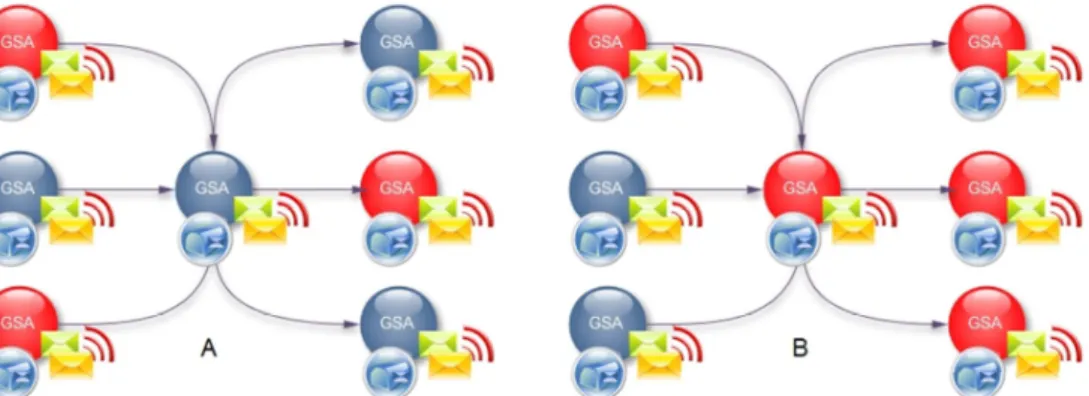
Figure 10 Possible representation of two surrounding observations for the central agent. ... 73

Figure 11 Local diagnostic adaptation to a fault propagation. Green arrows denote information condition exchange, while red arrows point the fault propagation path. ... 74

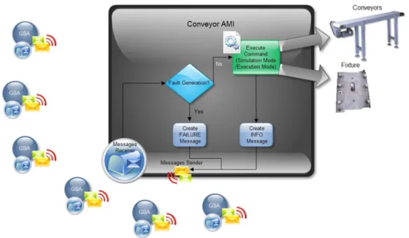
Figure 12 Conveyor AMI interactions and operation. ... 79

Figure 13Scara Station AMI interactions and operation. ... 80

Figure 14 Broker Agent interactions and operation. ... 81

Figure 15 Interactions to ADD or REMOVE a Neighbour. ... 85

Figure 16 Representation of a possible neighbourhood scheme for the NOVAFLEX cell. ... 86

Figure 17 Messages exchanged between GSA and the Broker Agent. ... 87

Figure 18 Skill instantiation flowchart. ... 89

Figure 19 Orchestrator flowchart. ... 90

Figure 20 Abbreviated message in a Pick and Place operation. ... 92

(24)

Figure 22 Workflow Manager Neighbourhood before and after the execution of a move Skill. ... 95

Figure 23 Abbreviated message exchanged during the change from position 1 to position 2. ... 96

Figure 24 Workflow Manager flowchart. ... 97

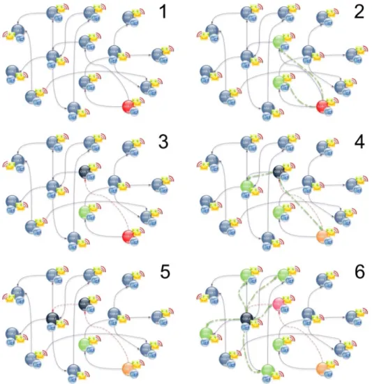
Figure 25 Example of a GSA network Fault propagation... 98

Figure 26 Fault Propagation Manager Flowchart. ... 99

Figure 27Message exchanged between GSA and the graph designer. ... 100

Figure 28 GSA interface... 101

Figure 29 Learning algorithm interface. ... 102

Figure 30 Example of a GSA network Status propagation (trace arrows). ... 103

Figure 31 Message Sequence to inform change in status. ... 104

Figure 32 A matrix representation. ... 106

Figure 33 Container Management interface... 108

Figure 34 Message exchange between the Container Manager and the graph diagnostic designer agent. ... 109

Figure 35 Network Generator Agent interface. ... 109

Figure 36 Message exchange between the Network Generator and the fault simulation target. ... 110

(25)

25 1 INTRODUCTION

This chapter introduces the research problem which based and substantiated the implementation

of this thesis. Moreover a brief description and summarization of the organization of the document is

presented.

1.1 Research Problem

The recent socio-economic crisis along with the normal unpredictability of the business environment challenges the emergence of new production trends and paradigms to cope with these highly dynamic, unpredictable and demanding economies. Therefore, diagnostic is becoming a crucial pillar in enterprises sustainability.

Through time the market requirements are becoming more demanding. Small and medium size industries tend to focus their target customers and core business as a strategy to deal with market competitiveness. Enterprises have to be increasingly prepared to quickly respond to sporadic market opportunities. Near zero device downtime, production quality, low maintenance costs are now more important than ever, each minute with suspended production may be synonym of thousands of euros of loss.

(26)

26

to unique natural habitats and also to society. Even though major accidents are the most noticed, the medium to smaller accidents can represent a loss of millions [1].

Moreover mass customization, where each customer demands a personalized product, is nowadays a reality. This new customer’s demand shortened the products life cycles and increased the production requirements.

To address this scenarios research and development of distributed production paradigms have increased through time achieving nowadays a very significant importance. Its importance can be verified through the number of related projects from the European Framework Programmes (FP) and from other similar programs.

From FP4 the project DIAMOND (Distributed Architecture for Monitoring and Diagnosis) [3]. In FP5 DEPAUDE (Dependability for embedded automation systems in dynamic environments with intra-site and inter-site distribution aspects) [4] among others. More recently SODA, a Schneider Electric’s effort in this area, using Service Oriented Architecture (SOA) [5], and SOCRADES (Service-oriented cross-layer infrastructure for distributed smart embedded systems) [6] developed under the project SIRENA (Service Infrastructure for Real-time Embedded Networked Devices) [7], EUPASS (Evolvable Ultra-Precision Assembly Systems) [8], developed under the FP6. Disc (Distributed Supervisory Control of Large Plants) [9], IDEAS (Instantly Deployable Evolvable Assembly Systems), and SELFLEARNING (Reliable Self-learning Production Systems based on Context Aware Services). These are just a small sample of the research efforts in this area.

(27)

27

Distributed architectures are usually complex systems and consequently more demanding to diagnose, consequently classical diagnostic approaches are not usually prepared to cope with these new scenarios. Therefore a new distributed interaction-based diagnostic approach compliant with the complexity of distributed state-of-the-art architectures is presented. As base for a distributed diagnostic system the developed work also presents an agent-based interaction-oriented distributed architecture. Relying on generic device abstracting agents, the architecture is characterized by the high level of granularity, self-* capabilities and emergence of skills. The diagnostic system not only counts on the sensor information, but also uses the richness of interaction of complex systems to reason about the agent state. The diagnostic algorithm has the ability to co-evolve with the remaining system, through learning and adaptation to the operational conditions. Moreover, the idea is to foster the emergence of global diagnostic perspective through local diagnostic, which allow the perception of the fault evolution within the network.

The architecture is Multi-Agent System (MAS) based and uses the platform Java Agent Development Framework (JADE) implemented in the JAVA programming language. The agent technology was selected foremost because MAS architectures are the fundamental engines underlying components autonomy that support the implementation of behaviours, dynamic and open environments. Agents provide a proper way to consider complex system with multiple distinct and independent components. JADE is a framework FIPA compliant and can be distributed across various machines [10, 11]. Moreover the agent technology meets all the performance requirements of state-of-the-art architectures, as well as modern production paradigms.

(28)

28

1.2 Thesis Presentation

This thesis is organized in five main chapters: Introduction, State-of-the-art review, A diagnostic infrastructure for EPS, Implementation and Conclusion and future work.

The Introduction chapter briefly substantiates the research problem and describes the organization of the document.

The second chapter on State-of-the-art contextualizes the developed work within the existing manufacturing paradigms as well as surveys the classical diagnostic methods and discusses its importance in nowadays markets and economic environment. Moreover some supporting theoretical concepts on diagnosis, HMM and the philosophical approach of Evolvable Production (EPS) are presented.

The third chapter “A diagnostic infrastructure for EPS” details the hardware infrastructure, as well as presents the system and diagnosis architecture based on EPS paradigm. This chapter outlines the singularities of this work, and exposes the choices made to accomplish the desired system and architecture.

The fourth chapter presents the implementation that validates the architecture introduced in the third chapter. Each individual participating entity is fully detailed. The control system, communications between agents along with the diagnostic systems… are exhaustively described, as well as the system interface is briefly depicted. The validation process is also explained, through the clarification of the testing scenarios and the presentation of the achieved results.

(29)

29 2 STATE-OF-THE-ART REVIEW

In this chapter a review on the state-of-the-art of manufacturing paradigms, diagnostic in

distributed and manufacturing techniques is presented along with an overview on Hidden Markov

Models and random graphs analysis.

2.1 Manufacturing Paradigms

The first references to manufacturing flexibility report to Diebol (1952). Diebol recognized flexibility as an essential part for medium and short-run manufacturing of discrete parts [12]. In the past, the manufacturing world was ruled by the economy of scales. Mass production and full utilization of plant resources were the way to maximize profit. This philosophy led to inflexible and not easily reconfigurable shop floors.

(30)

30

flexibility, elimination of inventory excess, shortened lead-times, and higher level of quality, industrial analysts popularized the term lean manufacturing. In the early 90s a study was carried out to study how US industrial competiveness would or might evolve during the next 15 years. One of the study results was the introduction of the agile manufacturing system (AMS) concept [14].

Similarly in the early 90s other paradigms emerged. Lean manufacturing system is one that meets high throughput or service demands with limited supplies, and with minimal waste. The main repercussion of lean manufacturing is the way that production is organized and managed. It influences the all production process, from the suppliers to the customers. The most important idea behind lean manufacturing is avoiding waste [15].

Agile manufacturing is a step further relating lean manufacturing, since lean manufacturing deals with things that cannot be controlled [16]. Agility influences different areas of manufacturing, from management to shop floor. The agile manufacturing desire the integration of design, engineering, and manufacturing with marketing and sales, which can only be achieved with information and communication technology (ICT) [15]. Agile manufacturing is a response to complexity caused by the constant changing’s, whereas lean manufacturing is a response to competitive pressure with limited resources.

(31)

31

In the last decade’s globalization has become a reality. The economy is no longer national but global and with it, new market demands have emerged. Society wants high quality products at low prices, highly personalized which implies short life cycles. To respond to this new market demands, enterprises had to start focusing their core business [21]. Though, in order to respond to short-term business opportunities enterprises had to start develop networking, to share knowledge and form partnerships [22]. The concept of reconfigurable manufacturing system (RMS) was introduced [23, 24] to respond to this new market oriented manufacturing environment [25]. A RMS is designed to conciliate both productivity and ability to react to changes. RMS capacity and functionality can change over time while the system reacts to new market circumstances. As described in [23] “A Reconfigurable Manufacturing System (RMS) is designed at the outset for rapid change in structure, as well as in hardware and software components, in order to quickly adjust production capacity and functionality within a part family in response to sudden changes in market or in regulatory requirements.”

On a study of Manufacturing 2020 [26], the RMS concept was identified as the number one priority technology for future manufacturing and one of the six key research challenges. A survey was also conducted by experts in 1997 [27], which tried to explain the experiences to date with FMS and identifies their accomplishment and failure [25].

(32)

32

Agent technology provides a natural way to implement and design distributed manufacturing systems. Therefore MAS architectures are a appropriated technology to implement modern manufacturing paradigms. CoBASA [15] and ADACOR [31] are two examples of recent manufacturing paradigms implemented through MAS architecture. CoBASA is a multi-agent based reference architecture that support fast adaptation and changes of shop floor control architecture with minimal effort [15]. ADACOR is an agile and adaptive manufacturing control architecture that increases agility and flexibility of enterprises, dealing with the need for the fast reaction to disturbances at the shop floor level [31]. In [32] a complete review in agent-based systems to manufacturing is presented.

2.1.1 Evolvable Production Systems

Evolvable production System (EPS) or Evolvable Assembly System (EAS) is a concept very related with RMS [33, 34].

There are two fundamental guiding principles in EAS/EPS [35-37]:

− “Principle 1: the most innovative product design can only be achieved if no assembly process constraints are posed. The ensuing, fully independent, process selection procedure may then result in an optimal assembly methodology.”

− “Principle 2: Systems under a dynamic condition need to be evolvable, i.e., they need to have an inherent capability of evolution to address the new or changing set of requirements.”

As major differences between EPS and RMS, it is important to stress that EPS focuses on adaptability of components as well as on re-engineering needs of the assembly system. Regarding modularity, EPS present a much higher level of granularity, since the abstraction unit can be the desired one. It also ensures the system robustness when the system is facing disturbances.

(33)

33

artificial intelligence (AI), complexity theory, system theory and cybernetics, artificial life including swarm theory and mobile robots and autonomic computing, to cope with complexity [38].

EPS systems rely on many simple, decoupled, intelligent, proactive and re-configurable modules or entities, which through self-capabilities or physical module addition allow evolution of the manufacturing system. These represent the main requisites for pluggable, evolvable and reconfigurable system [39]. Evolvability implies the capacity of co-evolving in line with the changing requirements and the environment. Higher level functionalities emergence is fostered through coalitions and interactions between entities. When considering a group of entities, different elements combinations can originate a variety of higher level functionalities.

In EPS, plug ability is ensured with none necessity of re-programming [34], whereas self-* capabilities concerning installation, management, healing, learning, diagnostic and other features are used to increase the system autonomy and minimize user interaction. One of the requirements for the modern emerging manufacturing paradigms is also making the manufacturing systems more user-friendly [40].

The main characteristics of an EPS system include: distributed control, modularization, intelligent and open architecture as well as a comprehensive and multi-dimensional methodological support that embrace the reference architecture [35]. Moreover, control solutions for EPS must deal with the following aspects:

− Support for integration of modular components, during stationary state and normal production.

− Product changes.

− Fluctuations in demand.

− Provide support for operative phase.

(34)

34

2.2 Diagnosis

2.2.1 Historical Introduction

In the 60’s there was a progressive evolution at the level of goods and services consumption. Associated with this evolution a new demand, regarding the quality price relation, emerged. The need to reduce manpower due to the high salaries, and the search for less monotone jobs, by the employees, were some of the causes to the expansion of process automation.

With the appearance of microprocessors, process automation started to overlap manpower in the production lines. The increased production capacity and the low maintenance costs, compared with the labour costs, allowed broadly higher profits. The development of sensors and actuators, the understanding of the theoretical fundamentals at the automation level, along with the appearance of new information technologies (IT) had a preponderant role in the development and utilization of the diagnostic methodologies. The computer control has brought enormous advances in terms of complex systems. Low level actions performed by specialized operators were successfully replaced by automation control applications. To supervise the autonomous execution and prevent failures, diagnostic methodologies and fault supervision were introduced. A historical survey on diagnostic methodologies development is a multi-disciplinary research area which has to face some literary dispersion [41].

Since early times that the use of diagnostic systems was considered a necessity. Industrial statistics shows that despite low frequency, major industrial disasters have an enormous social, financial and environmental impact. Nevertheless, the medium and small size accidents that originate small injuries and little material damage, cause losses of billions due to their high frequency occurrence [1]. To face this scenario, the control and management of abnormal events, become a priority.

(35)

35

Production downtimes and industrial accidents are seen as a source of pollution and waste of energy. These are determinant elements in the lower longevity of expansive equipment.

There are two main areas, through which the diagnostic systems can be developed, hardware redundancy and analytical redundancy. [42]. Hardware redundancy usually relies on a voting system and multiplication of physical devices, in order to detect the location and origin of the fault. This type of diagnostic is however characterized by the high costs that the extra hardware represents. The analytical redundancy uses in turn, relations between system variables through which the system diagnostic is possible.

The early 70s mark the begging of analytical redundancy-based fault research. Beard (1971) developed an observer-based fault detection scheme at MIT. Jones (1973) continued the development of his work [42]. Their work originated a fault detection filter called Bear-Jones. Relatively at the same time statistical approaches to fault diagnosis were first used by Mehra and Peschon (1971) followed by Willsky and Jones (1974). In the year of 1975 Clark, Fosth and Walton used the Luenberger observer for the first time. In 1980 a residual generation scheme based on consistency checking on the system input and output over a time window was introduced by Mironosky [42]. In the late 80s a group of AI researchers proposed a diagnostic method based on First-Order logic. This method utilizes an inference process to identify possible fault components.

Quantitative fault diagnosis methods appeared during the 80s, such as observer-based approaches, parity relation methods and parameter estimation methods among others. In 1991 a Steering Committee called SAFEPROCESS (Fault Detection, Supervision and Safety for Technical Processes) has been created within International Federation of Automatic Control (IFAC). In 1993 SAFEPROCESS became a Technical Committee within IFAC due to its importance [42].

(36)

36

More than ever, diagnostic and fault detection are a very important research field in engineering and particularly in manufacturing systems, since it has implications in a variety of domains like sustainability, efficiency, maintenance and security. Moreover, in critical systems like nuclear plants, aircrafts, submarines and medical devices, among others, the correct and anticipated fault detection is mandatory, otherwise a fault can result in loss of human beings and significant environmental impact [43].

The inevitable development of new technologies and the emergence of new paradigms, led to the appearance of new diagnostic methods, with the purpose of making the system even more productive, efficient and with less and smaller downtimes.

2.2.2 Preliminary Concepts

According to Bocaniala and Palade [42] a “fault is the abstraction of an abnormal event that causes unexpected changes in the system normal operating state”. A failure represents a serious breakdown of a component or function that implies a serious deviation in the behaviour of the whole system. Although both terms present similarities, a failure is a much more catastrophic event, whereas a fault may not affect the functioning of the overall system.

Isermann in [44] further classifies faults according to time dependency.

− Abrupt fault (stepwise): The fault is felt immediately, and brings the system very close to the limit of acceptable behaviour.

− Incipient fault (drift-like): Its effects increase through time, in the beginning it is almost unnoticeable.

− Intermittent fault: Its effects are noticed in discontinuous periods of time.

(37)

37

of the important characteristic of this type of systems is automatic reconfiguration when malfunctions are detected and isolated.

A diagnostic system operation can be decomposed into three main tasks, the fault detection which indicates the occurrence or not of a fault, fault isolation, to determine the fault location and fault identification to estimate the fault nature and significance [42].

State-of-the-art methodologies have to face new levels of complexity presented by the distributed characteristic of modern architectures and paradigms [45]. Despite the new challenges faced by modern diagnostic methodologies it is consensual that all diagnostic system should present a number of important requirements [1, 46].

− Quick detection and diagnosis: Concerns the commitment between the quickly faults detection and the system tolerance to noise during normal operation. These two desired characteristics have two conflicting goals.

− Fault isolation: Defines the capability of the system to distinguish between different diagnose failures. This characteristic also presents a commitment that has to be made regarding the isolability and the rejection of modelling uncertainties.

− Robustness: Represents the system capacity to cope with noise and uncertainties, maintaining a reasonable acceptable performance.

− Novelty identifiability: Is the system ability to identify and distinguish between known and unknown failures that might occur. Although the detection of a faulty state is a basic requirement, the identification of unknown events is much more complex once the diagnostic system was not designed to recognize such fault. Is also important to avoid the classification of unknown failures as a known one. Despite the difficulties novelty identification is a desirable characteristic.

(38)

38

− Adaptability: Operation conditions can change not only due to disturbance but also because of environmental conditions, natural detritions and manufacturing requirements. Therefore the diagnostic systems must be adaptable in order to evolve with the changes.

− Explanation facility: Represents the ability to explain the fault origin and path that led the system to the current faulty state. This is an important requirement to keep in mind, once it is through this characteristic that the systems can provide an explanation and assistant to the maintenance operator.

− Modelling requirements: The system must be modelled in order to maximize the diagnostic efficiency, by decreasing the model complexity.

− Computational requirements: Computationally heavy models may affect the system performance. Therefore the diagnostic model should be correctly balanced between complexity and computational power, with the aim of be efficiently and correctly performed.

− Multiple fault identifiability: represents the system capacity of relate and manage different and multiple faults scenarios.

2.2.3 Diagnostic Systems Classification

The scientific community, mainly of fault detection and isolation community (FDI) and diagnostic community (artificial intelligent and computer science background), are responsible for the research and development of diagnostic methodologies, is not very clear regarding the classification of diagnostic methods.

According with [47] the diagnostic systems may be categorized according two approaches, regarding the initial knowledge of the system.

− First principles approach: The known information respects the system description, along with the observation of the system behaviour.

(39)

39

Milne in [48] presents a number of strategies to build diagnostic systems based on knowledge such as structural, behavioural, functional and pattern matching. Knowledge can equally be based on past experiences and acquired information during the process utilization. In this case the classification is shallow, compiled, evidential and process history-based. More information about classification of a priori knowledge can be found in [48, 49].

In [50] diagnostic methods are divided in model-based fault detection methods and fault-diagnosis methods. The model-based fault detections methods are:

− State output observers,

− Parity equations.

− Identification and parameter estimation.

− Bandpass filters.

− Spectral analysis.

− Mean and variance estimation.

− Likelihood-ratio-test, bayes decision.

− Run-sum test, two-probe t-test.

Whereas the fault-diagnosis methods are composed by:

− Geometrical distance and probabilistic methods.

− Artificial neural networks.

− Fuzzy clustering.

− Probabilistic reasoning.

− Possibilistic reasoning with fuzzy logic.

(40)

40

More recently Venkatasubramanian has proposed a new classification, Figure 1, which can be found in [1, 51, 52].

According to Venkatasubramanian the diagnostic methods can be divided in quantitative methods, qualitative methods and history-based methods. This classification was designed according with two of the main characteristics of the diagnostic systems.

− Type of Knowledge.

− Type of diagnostic search strategy.

The strategy of the diagnostic generation is function of the knowledge representation scheme, which in turn depends on the a priori system information.

(41)

41

Quantitative information model-based relies on information generated from the mathematical relation between the input and the output of the system (residues), Figure 2, which are evaluated by a mathematical function that describes the system.

A model-based system is composed by the following main stages [53].

− Residual Generation: computation of input and output of the system to generate residual signal. It uses a system model relating the variables, which is use to check inconsistencies in order to detect faults.

− Decision Making: consist on examine the residuals for fault likelihood and decide if any fault has occurred. Moreover, the correct fault detection is then complemented with the fault isolation procedure to locate the fault.

In qualitative reasoning three different types of reasoning can be addressed. Abductive reasoning implies the generation of explanations for the observations. This type of reasoning is characterized by the number of answers, once for one observation a set of answers can be obtained. The way to choose between answers is by selecting the most probable one. Inductive reasoning is characterized by the establishment of rules categories or concepts that are inferred from a set of representative data. Finally, default reasoning is based in the manipulation of data. It is ideal to use when data need to be updated and override.

(42)

42

Contrasting with model-based approaches, where a prior knowledge of the systems is necessary, in history-based models the requested information is only historical known system information. There are different ways to draw knowledge and build the model through historical information. These methods are used for feature extraction [52]. The development of expert systems based on knowledge, was a first attempt to capturing the knowledge in order to generate conclusions [51].

In this document the author will follow the classification depicted in Figure 1 and [1, 51, 52].

2.2.4 Diagnostic Methods Overview

As it was stressed before, diagnostic classification can assume a variety of forms according to the author background and beliefs.

2.2.4.1 Quantitative Model-Based Methods

In the automated control area, fault detection problems are solved through FDI models. All FDI model are two step models, residual generation and decision making, as it was pointed out in a previous section.

Analytical redundancy methods rely on mathematical methods which represent the physical system behaviour. The idea is to compare the behaviour of the real system against the previously created model, and check for inconsistencies [54].

(43)

43

method for identify parity relation, which are used to build a residue generator based on the parity space. An adaptive monitor method is also presented.

The key in fault detection and isolation through observers is the generation of a set of residues that ensure the correct detection and fault recognition, even in the presence of unknown scenarios. In normal operation mode, all the observers must produce small residues, whereas in the case of a fault occurrence the observer sensitive to the fault should present a much higher residue value. Moreover, each single fault should present a unique pattern in order to allow fault recognition.

A Kalman filter consists of a set of mathematical equations which provide an efficient computational mean to estimate a linear process state, in order to minimize the mean square error. This type of filter enables the estimation of past, actual and future states, even not knowing the precise nature of the modulated system [58]. In [59] a Kalman filter based fault diagnostic system on a networked control system is presented. Kalman filter theory is used to compute filter parameters. Through the obtained values a filter is built and its outputs are used to generate the residues to diagnose the sensor and actuator faults.

If the process or any process related measure is not linear, then an Extended Kalman Filter (EKF) should be used [58]. A use case of an EKF used to detect faults is presented in [60]. The filter is used to generate residues through the comparison between state estimation and real measures that are analysed to detect the occurrence of faults.

2.2.4.2 Qualitative Model-Based Methods

Diagnosis concerns the deduction of the structure from the behaviour and for this to be possible, interpretation and reasoning over the recovered data is necessary. This process enables the construction of relations between causes and effects. Those relations can be represented through a Signed Digraph (SDG).

(44)

44

link between two nodes, which implies the relation between the cause and effect. Each node in the SDG corresponds to the deviation from the steady state of a variable [51].

The diagnostic of multiple failures is a complex problem, once the number of combination might exponentially grow with the number of failures. In [61] SDG based algorithm for multiple fault diagnosis is presented. Knowledge based consisting of knowledge about the process constraints, maintenance schedules among other types of knowledge is used to overcome the low resolution of the SDG. The computational complexity is controlled assuming that the occurrence probability of multiple failure scenarios decreases with the number of failure involved [61]. In [62] a method using SDG to calculate the optimal location of the sensors in order to improve the diagnostic result is introduced.

Fault trees are methods that are usually used to perform analysis of security and confidence in the system. Fault trees are logic trees that propagate primary events or faults up to the higher levels [51]. They are usually built by node layers. Each node is associated with different propagation logic. It is also a good method to prevent or identify failures before they happen, despite the very time consuming and expensive processing in the case of complex trees. Approximations can be used to contour the problem, but they will have repercussions in the precision. Since they use combinatorial logic, fault trees analysis (FTA) is a method that allows fault analysis. Using this methodology, different logic nodes can be applied (OR, AND, XOR), instead of the traditional OR used on Digraphs [63].

(45)

45

heterogeneous data, in order to generate a processing plan in real time [65]. QPA is a methodology based in the cooperation between qualitative physics and expert systems.

Another form of model knowledge is through the development of abstraction hierarchies based on decomposition. This type of decomposition aims the representation of the all system behaviour, through the laws that rule the subsystems. There are some important principals regarding the system decomposition. The non-function-in-structure principle implies that the laws of the subsystems may not depict the whole system. Other important principle is the locality principle that respects the incapacity of a specific part of the system laws to represent other parts of the system.

The system decomposition can be divided in two types:

− Structural: “Specifies the connectivity system information and its subsystems.”

− Functional: “Specifies the output of a unit as a function of its inputs.”

Diagnostic can be regarded as a top-down search, from the highest level, where the functional systems are considered, to the lower and individual units level, where individual unitary functions are analysed [51].

In [66] a Probabilistic Abstraction Hierarchy (PAH) is introduced. Bayesian networks are used to represent different abstract hierarchies. A PAH model is represented by a tree where each node is associated with a class-specific probabilistic model (CPM). Data is only generated at the leaves of the tree, and a model basically defines a mixture distribution whose components are the CPMs at the leaves of the tree.

2.2.4.3 Process History Based Methods

(46)

46

necessary are interpreted by the inference engine [52], returning manageable conclusions. The strength of these systems is the knowledge, which at the same time can represent a weakness point whenever unknown conditions are verified. These situations are reported has faults. It is also important to stress that the rule-based knowledge does not represent the physical behaviour of the system.

The main advantages of its use are: an easy development, transparent reasoning, the ability to reason over a some uncertainty and the capacity to provide explanations for the provided solutions [67].

An expert system based on a set covering model is presented in [68]. This type of model is presented as a solution to the difficult problem of multiple and simultaneously faults. In a set covering model the subjacent knowledge to a diagnostic problem is organized according to the representation of disorders and manifestations, where the disorders are symptoms of the manifestations. In [69] a expert system that attempts to address some of the issues involved in bridging the gap between human and computer expertise. The system uses two types of knowledge one based on experience and other based on how the device to be diagnosed works.

(47)

47

Quantitative feature extraction methods-based can be divided in two major methods, statistical feature extraction from process data and neural networks. Within Statistical feature extraction from process data, principal component analysis (PCA) and statistical classifiers will also be referred.

The quantitative approaches essentially formulate the diagnostic problem-solving as a pattern recognition problem. Statistical methods use knowledge from a priori class distributions to perform classification.

Regarding Statistical feature extraction from process data, the future states of stochastic systems cannot be completely determined through passed states, present or future control actions. This limitation is a problem when dealing with systems with random disturbances. The system configuration in a probabilistic manner is a way of dealing with this difficulty. When the system operates in a normal state, the observation presents a distributed probability, otherwise with an abnormal event the system will present other values.

PCA is used to define from an orthogonal partition of the measurement space, two orthogonal sub-spaces: a principal component sub-space and a residual subspace [71]. This method is frequently used when huge and multivariable data sets need to be reduced into a simpler form. In [72] a improvement in a PCA model is presented, through the selection of the personal computer that present the best variable reconstruction. One of the benefits is the à priori fault reduction, caused by non-correlated sensors in the module.

Following a classification approach a diagnostic system can be faced as statistical pattern classifier. The Bayes classifier is an optimal classifier when classes are Gaussian distributions and the distribution information is available. The distance based classifiers use distance metrics to calculate the distance of a given pattern from the means of various classes and classify the pattern to the class from which it is closest. The more basic distance base classifier is the Euclidean classifier. There are also the piecewise and quadratic classifiers [52].

(48)

48

behaviour [73]. An ANN is composed by a group of artificial neurons distributed by layers. The input and output layers represent the system input and output respectively. Moreover the dynamic of the modulated system is represented in the hidden layer. In order to perform the desired task, the ANN is trained with system dynamics representative data. Each ANN can be composed by an infinite number o neurons, however there has to be a compromise between the generalization capacity and the specificity of the network. In [74] a multi-layered feed forward neural-network approach is used to detect and diagnose faults in industrial processes. In this paper particularly it requires a system that is capable of observing multiple data simultaneously. The diagnostic system is basically composed by two-stage neural network. The first detects the dynamic trend of each measurement and the second one detects and diagnoses the faults.

2.2.4.4 Hybrid Methods

A single diagnostic system cannot possess all the desired characteristics. Therefore hybrid systems were developed to integrate more than one diagnostic methodology, which can be quantitative, qualitative or history-based, as a way to suppress the individual diagnostic methods limitations. Some work on hybrid architectures has been developed through the last years. The two-tier approach by Venkatasubramanian and Rich [75] using compiled and model-based knowledge is one of the earliest examples of a hybrid approach [52]. Another hybrid diagnostic system, that relies on Hidden Markov Models (HMM) and dynamic systems models of discrete and continuous time, able to deal with unknown behaviours is introduced in [76]. This capacity allows the diagnostic execution in systems where none assumption is made about the behaviour of one or more components of the system.

2.2.5 Diagnosis in Manufacturing and Distributed Systems

(49)

49

As it was pointed out in a previews section, new manufacturing paradigms are increasingly relying on MAS architectures, due to its distributed characteristics. In this context, a multi-agent based monitoring and diagnostic architecture for industrial components is presented in [77]. In this architecture each component has its own monitoring agent and a semantically distributed group of agents. Moreover a facilitator agent is responsible for the communication between the monitoring agent and the group of diagnostic agents. After processing the data the diagnostic is written in a blackboard. A facilitator agent is informed about the action and checks the blackboard for semantically or spatially conflicting diagnosis. The diagnostic approach uses a model-based combination of semantically and spatially distributed diagnosis and the use of KQML-CORBA (Knowledge Query and Manipulating Language) for implementing the architecture. Similarly a multi-agent diagnostic system where the knowledge is distributed over multiple agents, and each agent possess a model of a subsystem, as a solution to establish global diagnosis of large distributed systems is introduced in [78]. It also relies in a model-based diagnostic where the model knowledge is spatially and semantically distributed over the agents.

A multi-agent distributed intellectualized fault diagnosis system for artillery command system is presented in [79]. Fault diagnosis system based on agent is constructed to realized fault diagnosis on complex system by make use of agent’s basic character and multi-agent system’s integrated ability. In [80] the handling of sensing failures and work on distributed sensing recovery is presented. Sensor recovery strategies along with considerations about the problems raised by its application in multi-agent platform are discussed. The diagnostic is achieved through a primary data structure EHKS (Exception Handling Knowledge Structure) that is used by the error handler. As a fault is detected a runtime exception is generated and an EHKS is filled with information which will be used for classification and recovery by the error handler.

(50)

50

the problem. The causal model acts as a sort of map, which allows the diagnostic to progress from easily detectable symptoms to more precise diagnostic hypotheses.

A decoupled and distributed SOA architecture that relies on DPWS technology to abstract the system entities is introduced in [82, 83]. The architecture implements a diagnostic system targeting low cost devices with low processing power and memory, performed through fault related structure knowledge of the domain. Diagnosis at the device level explores ACORDA, a recent prospective logic engine. The ACORDA engine assesses future states and support postponing abductive decisions until the arrival of new data from the realization of experiments.

A web-based multilayer distributed fault diagnosis system for remote diagnosis is discussed in [84]. The described architecture is a data-driven system. Therefore the knowledge learning process extracts expert knowledge from confirmed faults, using various intelligent data mining technologies such as rough set, artificial neural networks and decision trees. The case-based reasoning diagnostic mechanism consist on three main phases: choosing diagnosis parameters, performing diagnosis and saving diagnosis results.

A diagnostic system for heterogeneous manufacturing environments is presented in [85]. The diagnostic knowledge is modelled in terms of causal relation between diagnostic attributes associated with manufacturing processes. The binary causal relations are meshed via their common attributes into a network. An attribute corresponding to the effect in one causal relation can equally correspond to the cause in another causal relation in a uniform manner. A cause-and-effect diagram only depicts the causes of each individual symptom, although the information is complemented through an influence graph, which concerns the relations between symptoms as well as with the relations between causes and other symptoms caused by those same causes. The diagnostic mechanism applies a probabilistic inference method to the influence graph.

(51)

51

on-line and is achieved by comparing the actual system response with the optimal control sequences provided by the first order petri net. In the occurrence of a faulty event a diagnostic procedure is triggered and a recovery action is further imposed.

In [87] a combination of three diagnostic methods in order to diagnose completely the operational faults of a manufacturing system is introduced. The diagnostic systems are based on fault tree analysis as well as in logic and sequential control of manufacturing systems by programmable logical controller.

An implementation of an integrated diagnosis system in a manufacturing systems is particularly presented in [88]. The diagnostic is implemented through an expert system. Like in other expert systems, the knowledge can be physical or experimental. In [89] a benchmark manufacturing cell and some experiences of designing supervisors and diagnosis using the Ramage and Wonham framework are discussed. A fault-identification method that is based on nonlinear dynamic model of a robot manipulator is introduced in [90]. A nonlinear observer is used to identify a class of actuators faults after the detection of the fault by other method.

Consensus in a network is a recent approach and can represent an important parameter to account in network distributed diagnosis models. A fault consensus in a network of unmanned vehicles is presented [91]. Each vehicle is equipped with an interactive multiple model algorithm based FDI, as well as a consensus filter. An interactive multiple model based FDI algorithm provides a quantitative measure on the probability of a fault in the network that can be used for fault consensus. A consensus filter in each vehicle generates probability of a current mode of operation using the local probabilities as well as probabilities generated by neighbour’s vehicles. In this proposed algorithm, vehicles can detect faults that are not observable through their local measurements.

(52)

52

dependent, which prevents the utilization of the same diagnostic model in other systems. Moreover, the addition of new components, without reprogramming the system is also a feature rarely taken into account along with the fault propagation effects and real time network diagnostic adaptation.

The next section will present requirements and characteristics that must be accomplished when diagnose EPS systems.

2.2.6 Diagnosis on EPS

As it was already detailed, future manufacturing paradigms rely in small intelligent devices. The distributed nature of those systems requires an extra attention regarding diagnosis. Despite the distributed and decoupled nature of EPS along with its reliability on self*-capabilities, a diagnostic system for EPS follows the accepted requirements for any similar system. In [46] some requirements are presented such as early fault detection and diagnosis, proper fault discrimination, robustness, identification of multiple faults, fault explanation, adaptability among others.

Each individual intelligent component participating in an EPS architecture is expected to detect and react in real time to faulty scenarios and environmental changes. Self-* capabilities related with diagnostic should be used to perform short, medium and long term analysis. Short terms analysis grants reaction and capture of catastrophic faults, and unexpected events. The purpose of medium and long term analysis is the prediction of future events [39]. Due to the decoupled and distributed nature fault propagation and multiple fault identification, may become a hard problem to tackle [40]. Nevertheless, the communications and interaction capability of the individuals plays a very important role in the resolution of these challenges.

(53)

53

to a full manufacturing plant, according to the desired granularity. It is of major interest not only have individual diagnostic information, but a system diagnostic perspective revealing fault propagation through the network, modules dependencies along with multiple fault origin detection.

A diagnostic system compliant with EPS should also present evolvable capabilities in order to adapt its behaviour according to changes, and preserve functionalities even in scenarios where some part of the diagnostic infrastructure is not working.

2.3 Hidden Markov Models

Hidden Markov Models (HMM) were introduced in late 60s and early 70s and were firstly described in a series of statistical papers by Leonard E. Baum and other authors. HMM is very appropriated methodology to perform pattern recognition, particularly speech recognition [92-94]

An HMM [93, 95] is the following triplet:

) , , ( π

λ = A B

where A is a N×N matrix (N is the number of states in the model) denoting the state transition probabilities:

ij i t j

t

S

q

S

a

q

P

(

₊₁

=

|

=

)

=

B is an N×M matrix (M is the number of observation symbols) that encloses the observation probabilities:

)

(

)

|

(

O

k

q

S

b

k

P

_t

=

_t

=

_i

=

_i

(54)

54

In this context, a HMM can be considered a finite state machine where transitions between states are probabilistically driven (the probability of transition to another state given the current state).

When handling HMMs there are three fundamental assumptions [96]:

− The Markov Assumption - the next state is only dependent on the current state and the observations (valid for first order models as the one considered).

− The Stationary Assumption - the state transition probabilities are independent of the time at which they occur.

− The Output Independence Assumption - the current observation is independent of the previous observations.

Additionally HMM support the resolution of three main problems [93]:

− “Problem 1: Given the observation sequence O = O1 O2 …OT, and a model λ =

(A, B, π), how do we efficiently compute P(O|λ), the probability of the observation sequence, given the model?”

− “Problem 2: Given the observation sequence O = O1 O2 …OT, and the model λ,

how do we chose a corresponding state sequence Q = q1 q2 …qt which is optimal

in some meaningful sense (i.e. best “explains” the observations) ?”

− “Problem 3: How do we adjust the model parameters λ = (A, B, π) to maximize P(O|λ)?”

The resolution for problem 2 that aims the discovery of the state sequence most likely to be produced by the given observation sequence, can be solve through the Viterbi algorithm, whereas the Baum-Welch algorithm can be used to solve the third problem which is coincident with the implementation of the learning process. Through the insertion of observation sequences the algorithm adjusts the parameters λ in order to best describe the observation sequences.

(55)

55

doubly embedded stochastic process with an underlying stochastic process that is not observable. An observation represents a probabilistic function of the state. HMM are adequate to represent problems where the internal state is not known and can only be inferred through observations [98]. Therefore and in order to bridge the HMM with diagnostic applications a fault can be considered a hidden state of the system that can be inferred through the observations. Moreover, HMM have the ability to deal with incomplete information [99].

Although not very commonly applied to diagnostic purposes, in [98] a formalization of the diagnostic problem based on HMM is introduced. The implementation showed high accuracy when compared with an optimal solution based on Bayesian inference theory.

2.4 Random Graphs

Random graphs were first introduced in the late 50s by Erdós and Rényi through the Erdós-Rényi network. There are two types of construction of random graphs, with a fixed number of vertices [100]:

− Construction Method 1: “Each two vertices of the network are connected by an edge with probability p. Naturally, this edge is absent with probability 1-p.”

− Construction Method 2: “A given number L of edges connects randomly chosen pairs of vertices. One can realize this construction procedure by adding new edges one by one and repeatedly connecting randomly chosen pairs of vertices. In graph theory, this is called a random graph process.”