A Work Project, presented as part of the requirements for the Award of a Master Degree in Finance from the NOVA – School of Business and Economics
MarketOpolis: A Market Simulation based on Investors Decisions
A case Study on Apple Inc.
Pedro Alexandre Calheiros Souto Nº18211
A Project carried out on the Master in Finance Program, under the supervision of:
Professor Pedro Ouro Lameira
[2]
MarketOpolis: A Market Simulation based on Investors Decisions
A case Study on Apple Inc.
Abstract: This study aims to replicate Apple’s stock market movement by modeling major investment profiles and investors. The present model recreates a live exchange to forecast any predictability in stock price variation, knowing how investors act when it concerns investment decisions. This methodology is particularly relevant if, just by observing historical prices and knowing the tendencies in other players’ behavior, risk-adjusted profits can be made. Empirical research made in the academia shows that abnormal returns are hardly consistent without a clear idea of who is in the market in a given moment and the correspondent market shares. Therefore, even when knowing investors’ individual investment profiles, it is not clear how they affect aggregate markets.
[3]
“Chaos is merely order waiting to be deciphered”
José Saramago
Acknowledgement
[4] 1 - Introduction:
Scientific simulations and replications are being used ever since the Academic community found it difficult to test any model in the “Real World”. If the model fits in a “small and little scientific world”, then it is possible to apply it into reality. Nonetheless, modeling financial Markets nowadays, which are one of the most (if not the most) complex systems ever produced, does not have a clear-cut answer. It is open 24 hours per day, seven days a week, and managing more than $294 trillion dollars. Moreover, if securitized products and over-the-counter derivative markets are considered, the size of financial assets is estimated to be at least $693 trillion dollars.1
Throughout the Globe, Mutual Funds, Brokers, Pensions Funds, Hedge Funds, Insurance Companies, Investment and Commercial Banks, just to name a few, decide what should be the fair value of every asset (such as Stocks, Commodities, Interest Rates, Future contracts, Exchange Rates, among several others). Therefore, it is a great challenge to, not only define how markets behave, but also to predict future movements and the likelihood of certain events.
The present work relies on the will of making a market replication and its participants’ decisions. Thus, following the steps specified by several studies and as indicated by Kirilenko et al. (2011), it begins by defining what are generally the major investors’ decisions, based on the assumption that every market player, by himself, has a pre-defined reasoning when investing. That ruling is made by rational decision makers, based on all the available information, fully expressed on asset prices, under the Market Efficiency Hypothesis. Following that reasoning, and besides the fact that many investors have a much more complex decision tree and available resources when they are investing (such as macroeconomic and
[5]
equity research papers, as an example), this paper relies on the assumption that all factors affecting their decision are already taken into account on the security price.
The literature found on the current topic is far from being homogenous. As pointed out by Burton G. Malkiel (2003), “Revolutions often spawn counterrevolutions and the efficient market hypothesis in finance is no exception”. The market efficiency hypothesis theory stands for the impossibility of consistent “free lunches”. In other words, EMH assumes that markets incorporate all the available information right after any fundamental economic change occurs. As well described in Lo et al. (2004) “This is not an accident of Nature, but is in fact the direct result of many active market participants attempting to profit from their information.”2 Despite having several perspectives of what is efficiency (strong, semi-strong or weak)3, the condition for an efficient market is the price variation randomness and unpredictability, like a “random walk”.
Contrariwise, this traditional view has been questioned with multiple evidences that show lack of rationality of investors when making decisions. Abnormal movements such as, short-term momentum4, long-term reversal5, and event-based returns, that generate high and inexplicable volatility on asset prices relatively to their fundamental value, are just some of the possible and exploitable opportunities for any smart investor, as highlighted by Daniel, Hirshleifer and Subrahmanyam (1998).
2 (Lo, 2004)
3 Where Strong form of efficiency accounts for all the information known to any investor at time t (public, private and even inside trading cannot give any advantage to an investor); Semi-strong when prices reflect not only the past data but also all the information public (neither fundamental data such as earnings, balance sheet, etc. nor technical analysis can give higher risk-adjusted returns) and finally, weak form where asset prices already reflect all the historical data (Jensen, 1978)
4 Positive short-term autocorrelation between stock returns (Bodie, Kane, & Marcus, 2011)
[6]
Nonetheless, further studies (Fama, 1998) have questioned some of those exploitable behavioral biases due to transaction costs, “ex-post” or forward looking biased analysis, and poor or
inexistent measurement of the fair risk-return of most anomalies6. Additionally, some literature (Malkiel, The Efficient Market Hypothesis and Its Critics, 2003) argues that even if irrational choices are able to produce patterns that deviate from the fundamental value, they are short-lived as soon as smart investors start to exploit them.7 Thus, without having a prevailed theory, new approaches, like the “ADH – Adaptive Market Hypothesis”8, were introduced to reconcile these two unalike academic fields.
In short, the present paper aims to address some of the challenges presented above, by building a proxy of the main financial market players’ behaviors. If the proxy is good enough to understand who are the key responsible for market movements, it may be possible to predict price reactions following distinct investments, by anticipating their actions and subsequent effects. Therefore, I intend to contribute to the present literature by adding new proxies for investors’ decision strategies and enriching the discussion about the likelihood of price change prediction.
The additional parts of the paper are organized as follows: Section 2 presents the empirical framework and the assumptions made to formulate the model; Section 3 describes the investors and market characteristics (activation functions), and their interaction; Section 4 examines the key predictions and findings using an intraday data snapshot; Section 5 upholds a short
6“consistent with the market efficiency prediction that apparent anomalies can be due to methodology, most long -term return anomalies tend to disappear with reasonable changes in technique.” (Fama, 1998)
7 In Singal’Book (Beyond the Random Walk: A Guide to Stock Market Anomalies and Low-Risk Investing, 2003) it is shown the major market anomalies and what is the likelihood of exploiting them having a consistence (but theoretical) profit.
8“AMH is based on an evolutionary approach to economic interactions, as well as some recent research in the cognitive neurosciences that has been transforming and revitalizing the intersection of psychology and
[7]
discussion on the topic, not only on the downfalls of the model, but also on future improvements needed to what has been developed so far.
2 – Methodology: Data Sources & Assumptions
For investors’ modeling, 5 years of daily data of Apple US Equity have been used (from January 1st 2010 until 18th of June of 2015), combining last or closing price and volume. Nonetheless, since several important investors’ and market features have a shorter-term behavioral horizon, a snapshot over the last 140 days (from 2014/12/5 to 2015/6/18) was taken, using 1 minute intraday bar data, which includes the Open, High, Low, Close and Volume of the same security9. Therefore, even though all investors are modeled for the entire sample, their actions are only going to be presented and tested for the last 140 days.
The reason behind choosing Apple has to do with its high recognition, being one of the most well known companies in the World and having the highest Market capitalization globally. It is traded by the majority of the foremost institutional or individual investors, and it is almost a mandatory presence in the World’s most relevant portfolios. Additionally, contrarily to replicating a future contract, Apple is still heavily traded by the majority of the investors, whereas High-Frequency trading firms dominate future contracts10. So, while the present study does not capture the business specific aspects of Apple’s business model, it is undeniable that it is a concourse where the majority of investors are found, and hence, the possibility to study their behaviors.
Regarding the model’s framework, it is a sum of two parts. Firstly, the best empirical and studied proxies for investors’ decisions are defined. Though, these proxies are not related to investor profiles but with investment styles, meaning that the categorization is made by the type
[8]
of investment trigger (or investor’s activation function) and not regarding them being Pension or Hedge Funds. For simplicity, 7 investor style profiles are categorized: Market Maker, Tracker, Mutual Fund, Fundamental Investor, Momentum Investor, Speculator and Noise Trader. Secondly, after having well defined functions to describe investor behaviors towards price change, a description of the interaction between each other to replicate a live exchange market is undertaken.
Finally, the model’s success is tested using constant market shares for each group of investors. Here, market share or weights are defined as the quantity each individual investor is willing to transact in a given sample observation (which is, in this case, 1 minute). So Market Makers are responsible for 15%, Tracker for 30%11, Mutual Fund for 20%12, Fundamental Investor for 10%, Momentum Investor for 10%, Speculator for 5% and Noise Traders for 10%13.
Nonetheless, fixing weights during the entire sample does not take into account when investors are not interested in either buying or selling. Actually, investors’ market share should be variable in order to better capture flows in volume, due to reactions to price developments and available opportunities. Similar studies have been made, by checking individual audit trails (Kirilenko et al., 2011) to find out the real buyers and sellers on a given trade. However, the present study did not have access to such detailed data. Therefore, the model goes a step further by optimizing the market shares so as to assess the optimal weights that zero out the output gap or the mean squared error the investor’s proxies. The used method was unconstrained optimization.
11“On average ETFs represent approximately 30% of the total volume traded” Source: BlackRock & Bloomberg as of 30 September 2010
12“Mutual funds hold about 20 percent of the publicly traded stocks of U.S. corporations” (Mutual Funds and the U.S. Equity Market, December 2000)
[9]
Concerning model evaluation, 3 methods are used: Mean Squared Error/Mean Absolute Error; Output Gap, which is the difference between the model price and the real one; and Model Success, where the cumulative prediction success percentage is evaluated14.
Nevertheless, given the limitations on the resources available to an exact replication, some financial markets’ aspects were let down and certain assumptions were imposed to guarantee
the model’s feasibility. First, there is no evidence that investors only look to the stock price
when making investment decisions. This may be true for some smart and faster investors, when seeking for very short-term positions (or pure arbitrages), but it is not reliable for a mutual or a pension fund. In this case, when deciding to put a given percentage of their notional on a corporation’s equity, their allocation is driven also by the quality of the managing team, industry sector, size or any other qualitative reasoning. Additionally, “zero inside trading” is assumed, meaning that every investor has the same information at the same time and cannot predict future stock returns. However, this has been questioned by Kirilenko, Kyle, Samadi and Tuzum (2011) on their study about Flash Crash and assymetric information.
Secondly, for simplicity, the investors created are unbiased and do not have any monetary constraint, which implies that they will buy or sell the security if their investment trigger is activated. In addition to this, being unbiased investors also implies that they do not share any investment timeframe bias, which means that they will invest right away, regardless if it is during the opening bell, 5 minutes before earnings’ announcement or throughout a speech of the Federal Reserve. Obviously, the present assumption can jeopardize some findings, since the most relevant economic releases or any important macroeconomic events are pre-known by the market, and investors modify their holdings accordingly. For instance, market makers and smart
14𝑆𝑢𝑐𝑐𝑒𝑠𝑠 = {1 , 𝑖𝑓 𝑀𝑜𝑑𝑒𝑙 𝑔𝑜𝑒𝑠 𝑖𝑛 𝑡ℎ𝑒 𝑠𝑎𝑚𝑒 𝑑𝑖𝑟𝑒𝑐𝑡𝑖𝑜𝑛 𝑜𝑓 𝑅𝑒𝑎𝑙 𝑃𝑟𝑖𝑐𝑒
0 , 𝑖𝑓 𝑏𝑜𝑡ℎ 𝑝𝑟𝑖𝑐𝑒𝑠 𝑐ℎ𝑎𝑛𝑔𝑒𝑠 𝑑𝑜 𝑛𝑜𝑡 𝑚𝑎𝑡𝑐ℎ ⇒ 𝑀𝑜𝑑𝑒𝑙 𝑆𝑢𝑐𝑐𝑒𝑠𝑠𝑖= ∑ 𝑤𝑖𝑥𝑖
𝑛 𝑖=1
∑𝑛𝑖=1𝑤𝑖 ,
[10]
investors tend to underweight and become more conservative before earnings, or Federal Reserve meetings, as studied by Bernanke & Kuttner et al. (2003). This feature can indicate an upward trend on the supply side and a decrease in demand, leading to an unnatural (but rational) stock price movement that is not controlled by the present model.
Furthermore, by focusing only on their decision triggers, the model does not take into account what were (at the time of the sample beginning) the inventory or invested notional on a given stock. Therefore, it is possible that, for example, a mutual or a pension fund that is forbidden of short selling stocks most of the times, does it here because it runs out of available stocks in the inventory (and his decision trigger keeps saying that is a good selling point).
Moreover, since the snapshot sample is 1 minute data, the model has already partially excluded an undeniably important and growing market player – High-Frequency Trading Corporations15. By looking only to what has happened after 1 minute, millions of transactions and relevant movements are excluded, which can lead to wrong conclusions. As an example, events as earnings, FED press conferences, macroeconomic releases, or simply a flush (such as the Flash crash, marvelously highlighted in Kirilenko, Kyle, Samadi, & Tuzum, 2011) can have an impressive 1 minute range16 but a zero price change when the overall movement is observed (after 60 seconds).
Finally, given the available literature, there is still no clear evidence on how those HFT firms impact stock prices. For instance, the Wall Street Journal HFT journalist expert, Greg Laughlin,17 described that even though over the past few years the volume has grown tremendously, more and more High-frequency trading firms are becoming simply a faster and
15The work “The Flash Crash: The Impact of High Frequency Trading on an Electronic Market” go even deeper testing the power and the size of those players (Kirilenko, Kyle, Samadi, & Tuzum, 2011)
16 The difference between the high and the low of that particular minute: Hi/Low Range = High - Low
17 See “Insights into High Frequency Trading from the Virtu Financial Initial Public Offering” on
[11]
more electronic market maker or liquidity provider. Additionally, there is an important feature on HFT behavior that somehow is incompatible with the present model. Most of their business models are built on the assumption that they can quickly understand the market trend and supply/demand gaps and execute it with a fast electronic order to “fill the gap”, i.e., removing temporary market inefficiencies18. By assumption, this model has the rule/constraint that all investors have the exact same time to buy/sell, meaning that everyone is only allowed to send one (and one only) minute order to the market. Moreover, it is also important to notice the fact that the present study is not taking into account some other trading features: there is no possibility of over-bidding or offering quantities that do not match the real desired quantity (several trading firms have that strategy to increase the likelihood of having a fill); and market orders are always limited “fill or kill”19, so GTC orders (“good until cancel”) are not allowed. Even though there is no evidence that different market orders are likely to change prices, it is undeniable that they can influence the who is the receiver of the traded quantity20.
3 - Replication Model
In order to replicate Apple’s stock market movement (or any other market or security), the major players and their reaction functions to price changes need to be defined. Moreover, without a trading place or framework, the interaction between each other would not be possible. The first section will be dedicated to the market players’ description, followed by the Market/Exchange itself.
At this stage it is relevant to take a look at transaction costs. Regarding the costs investors face when they are investing, only two plain/fixed fee structures are assumed: 1 basis points for
18 (Kirilenko, Kyle, Samadi, & Tuzum, 2011)
[12]
Market Makers, Trackers and Smart Investors/Speculators and 10 bps for Mutual and Pension Funds, Momentum and Fundamental Investors. The first group is more worried about costs control due to their type of action: numerous trades, shorter-term and smaller oriented investment timeframe, squeezed bid-ask spread, among others. For the second ones, their main goal is finding longer-term and bigger profits, leaning on higher short-term costs but ensuring they get exact what they want/need to accomplish their investment decisions. However, since financial markets are way far from being a binary world, it is undeniable that it is possible that some players from the previous groups have other brokerage fees and plans (higher or lower, fixed or variable, etc.), either because they are big enough to have a special fee or because they hold a brokerage firm, among several other possible reasons.
3.1 - Replication Model: The players
Market Maker: 𝐴𝑐𝑡𝑖𝑣𝑎𝑡𝑖𝑜𝑛 𝐹𝑢𝑛𝑐𝑡𝑖𝑜𝑛 = ℱ(𝑣𝑜𝑙𝑎𝑡𝑖𝑙𝑖𝑡𝑦, 𝑖𝑛𝑣𝑒𝑛𝑡𝑜𝑟𝑦, 𝑣𝑜𝑙𝑢𝑚𝑒)
The recognition of the market makers’ role in any market is as challenging as crucial for acknowledgement of how markets behave. There are some studies about how different market makers act across all asset classes and among several countries. For the sake of the present work, 2 types were modeled: unbiased and biased Market Maker.
Generally, a market maker is a player that most of the time has an inventory of securities to manage and it is willing to provide liquidity to the market by quoting the bid and ask prices. Their profit comes, therefore, from short-term mean reversion and squeezing the bid-ask spread.21 The unbiased market maker has no opinion on the direction of the stock and it is permanently willing to actively quote both sides (bid and ask) of the security. Nonetheless, it is not blindly buying/selling his inventory: it has a volatility and liquidity dependent investment decision function. Thus, the quantity that the market maker is showing in each level is a variable
[13]
of the average volume of the security on the previous 60 minutes22. Although market makers are actively quoting for simplicity of the model, it is undeniable that the number of working levels23 is crucially dependent on past volatility both in reality and in the model. The reason is straightforward tough: as market makers’ profit comes mainly from mean reversion movements, they need to perceive how wide the security can trade in order to understand how much they are willing to risk on a position. So, if the volatility increases/decreases, they will widen/narrow their bid-ask spread accordingly.
Having their “quoting system” linked with volatility allows them to be protected from great flushes that may occur. Nevertheless, it is also important to stress that this protective/conservative strategy may lead to even bigger drops in price, as when market makers stop quoting and take out their positions, they are creating a huge pressure on prices (by removing most of the market liquidity).24
Regarding the biased market makers, the only difference to the previous ones has to do with their “opinion” about the direction of the market (derived from a more complex mean reversion
strategy or just their inventory managing policy). In short, although those players quote both sides of the market, they are more aggressive (or over-quoting) on one side25.
22 The 60 minutes average volume was picked randomly but supported by the volume time dependence theory, shown in several studies (Singal, 2003).
23 Where working levels stand for how many prices a market maker is actively quoting at the same time
24 In the present model Market Makers are just volatility and not inventory dependent and so they do not create a selling/buying pressure when there is a big move (they only wide out their orders creating a bigger bid-ask spread/gap). Nonetheless, this assumption it is rejected by the theory as seen on studies about the flash crash (Kirilenko, Kyle, Samadi, & Tuzum, 2011).
[14]
Tracker: 𝐴𝑐𝑡𝑖𝑣𝑎𝑡𝑖𝑜𝑛 𝐹𝑢𝑛𝑐𝑡𝑖𝑜𝑛 = ℱ(𝐴𝑝𝑝𝑙𝑒 𝑃𝑟𝑖𝑐𝑒 𝐶ℎ𝑎𝑛𝑔𝑒, 𝐼𝑛𝑣𝑒𝑡𝑜𝑟𝑦, 𝐶𝑎𝑝𝑖𝑡𝑎𝑙 𝐹𝑙𝑜𝑤𝑠)
Fifteen years ago, if any financial professional was asked if it was possible that passive investment would account for more than 30 trillion dollars26, it would be hard to believe. Indexing is a straightforward strategy that relies on the argument that “security markets appear
to be remarkably efficient in digesting and adjusting to new information.”27 If so, and if an investor misprices (due to transaction costs needed to exploit any anomaly) or cannot reach any prediction of market trend, the correct allocation of investments should follow the aggregate market as a whole.
The most common passive investment strategy is through Exchange-Traded-funds, the so-called ETF’s. Those financial products are nothing more than a basket of securities that belong
to any index. For instance, since the firm under analysis has the greatest market capitalization on the S&P 500, it may be possible to tell how those trackers work by looking to the SPY US Equity28.
According to the prospectus, trackers need to replicate the index by owning a basket of the holdings of the index, in the compatible percentage of the index’s market capitalization. Consequently, they need to regularly rebalance their portfolios in accordance to daily price changes. This can be observed in the present study. As an example, if all else equal, when the stock price of Apple increases/decreases, the percentage of Apple market capitalization relative the S&P will growth/diminish, and so does the need of the tracker to buy/sell the stock in order to fully track the index29. Following their prospectus, their activation function starts when the
26 Source: Investment Company Institute. 2013. 2013 Investment Company Fact Book: A Review of Trends and Activity in the Investment Company Industry. Washington, DC: Investment Company Institute. Available at
www.icifactbook.org
27 (Malkiel, Passive Investment Strategies and Efficient Markets, 2003)
28 See more information on State Street Bank & Trust Company website and prospectus (https://www.spdrs.com/product/fund.seam?ticker=SPY)
[15]
tracking error is, on average, approximately greater than 4 basis points. This way, any Trackers that participate in this model (S&P 500 tracker, MCSI World Index tracker, Technological S&P500 Tracker, Large Capitalization US Index tracker, among several others) will trade in accordance to the divergence between Apple’s performance and what they have in their baskets, which is where the constant threshold of 0.04% breaks, for simplicity.
Fundamental Investor:
𝐴𝑐𝑡𝑖𝑣𝑎𝑡𝑖𝑜𝑛 𝐹𝑢𝑛𝑐𝑡𝑖𝑜𝑛 = ℱ(𝐹𝑖𝑟𝑚′𝑠𝑓𝑢𝑛𝑑𝑎𝑚𝑒𝑛𝑡𝑎𝑙𝑠, 𝐿𝑜𝑛𝑔 − 𝑡𝑒𝑟𝑚 𝑚𝑜𝑣𝑖𝑛𝑔 𝑎𝑣𝑒𝑟𝑎𝑔𝑒𝑠)
Even though there is no clear cut answer for what it is the fundamental price of a security, it is relevant to add in the present analysis those who are investing based on a long-term horizon and low-latency data (such as industry/sector cash-flows comparison, long-term profitability, return on assets, or macroeconomic variables like the impact of economic growth, inflation or interest rates). Contrary to shorter-view investors, fundamental investors tend to analyze what the company was doing on a 2 to 5 year timeframe. Additionally, they want to hold investments for a long period of time instead of squeezing short-term trends, not sustained by the firm’s fundamentals. However, since it was assumed previously that all the available information is essentially reflected on the price, those investors are just looking to the longer moving average in order to remove any short-term “irrational exuberance”.30
Hence, fundamental investors were modeled in the following manner: if the security breaks the threshold of 20% above/below the 5 years moving average, they will sell/buy, respectively. Also, they will only increase their net position if it breaks another threshold, which is now 30% above or below.31 They will only close an open position when Apple price retraces to the
30“Irrational exuberance” is an expression used by the then-Federal Reserve Board chairman, Alan Greenspan, to signal that the market were somehow overvalued.
[16]
opposite entered thresholds (if sold at 120%/130% of 5 year moving average, they will buy back when it breaks 80%/70% of the same average and vice-versa).
Momentum Investor:
𝐴𝑐𝑡𝑖𝑣𝑎𝑡𝑖𝑜𝑛 𝐹𝑢𝑛𝑐𝑡𝑖𝑜𝑛 = ℱ(𝑝𝑎𝑠𝑡 𝑤𝑖𝑛𝑛𝑒𝑟 𝑎𝑛𝑑 𝑙𝑜𝑠𝑒𝑟𝑠, 𝑣𝑜𝑙𝑎𝑡𝑖𝑙𝑖𝑡𝑦 𝑎𝑛𝑑 𝑜𝑣𝑒𝑟𝑟𝑒𝑎𝑐𝑡𝑖𝑜𝑛)
In order to answer the question of market overreaction, research by experts in experimental psychology and market simulation has been conducted. Accordingly, Bont and Thaler (1985) found evidence that “most people “overreact” to unexpected (…) events.”32 Tough, it is relevant to include in the model those investors that diverge from the fundamental value theory and rely on past winner and short-term trends to decide where to invest.
Momentum investors were set in 3 groups, reflecting their timeframe investment: daily, weekly or monthly. The main difference between them is merely if they are looking to trade daily ins and outs, or considering a broader and longer-term perspective. The introduction of 3 levels of decision is based on, for instance, Fisher Black (1986) and Brett Trueman (1988) studies stating that some institutions/investors tend to trade excessively the same industries/stocks that are showing a short-term trend direction in different timeframes (daily, weekly, monthly and quarterly).33 Also, further studies (De Long, Summers, & Waldmann, 1990) have proved the designated “positive-feedback traders” actions’ have a tendency to overweight equities that had performed better in the past. Therefore, they all share the same investment procedure: they rank the daily/weekly/monthly top winners/losers, and then they buy the 90th percentile and sell the 10th. It is important to stress that the investors do not take into account their net positions, meaning that they can sell/buy the same stock in the entire sample period.
32 (Does the Stock Market Overreact?, 1985)
[17]
Mutual Fund:
𝐴𝑐𝑡𝑖𝑣𝑎𝑡𝑖𝑜𝑛 𝐹𝑢𝑛𝑐𝑡𝑖𝑜𝑛 = ℱ(𝑀𝑜𝑚𝑒𝑡𝑢𝑚, 𝑇𝑟𝑎𝑐𝑘𝑒𝑟𝑠 𝑎𝑛𝑑 𝐹𝑢𝑛𝑑𝑎𝑚𝑒𝑛𝑡𝑎𝑙 𝑆𝑡𝑟𝑎𝑡𝑒𝑔𝑖𝑒𝑠)
The introduction of these open-ended investment companies, which account of “more than 90% of investment company assets”34 is imperative. However, due to its heterogeneity, it is hard to state a simple rule to define how they operate. Not only they are one of the biggest players in terms of notional, but also as diverse and tailor-made as possible. Nonetheless, due to its construction, they all compete to have the highest returns to their clients.35 If they perform poorly for a long period, clients will move to their competitors or simply adopt a passive strategy by buying, for example, an Exchange-Traded Fund. Consequently, “Most mutual funds adopt styles that bunch around an overall market index, with few funds taking extreme positions away from the index. When funds deviate from the index, they are more likely to favor (…) high past return over low past return.”36
Following the literature, Mutual Funds investment triggers are, somehow, similar to a combination of 3 already defined investors: Trackers, Momentum and Fundamental Traders. The explanation is then, straightforward: if they want to follow a common benchmark, they will rebalance their portfolios on the same manner as Trackers (if a given security is trending up, they buy it in order to keep the basket similar to the index they are tracking, in percentage of their market capitalization). Likewise, this paper introduces a broader number of funds, selecting those that, besides following the Index, are also driven by momentum or fundamental strategies. Therefore, the Mutual Funds’ activation function is equal to a combination of what those 3 strategies are doing in a given minute (amplifying their movements). Nonetheless, the 3 strategies should not have the same percentage. Even though there is lack of strong evidence
[18]
on what is the accurate percentage that each of these strategies represent on the overall group of mutual Funds, for the purpose it was attributed 50% for trackers, 35% for the momentum strategy and 15% for fundamental strategies37.
Speculator & Noise Traders: The introduction of these last 2 types of investors comes from the idea that by looking to the current volume of any security, there must be more investors out there trading based on investment triggers that are beyond the previous investor classes.
Speculator: 𝐴𝑐𝑡𝑖𝑣𝑎𝑡𝑖𝑜𝑛 𝐹𝑢𝑛𝑐𝑡𝑖𝑜𝑛 = ℱ(𝐼𝑛𝑡𝑒𝑟𝑛𝑎𝑡𝑖𝑜𝑛𝑎𝑙 𝐸𝑞𝑢𝑖𝑡𝑦 𝐼𝑛𝑑𝑖𝑐𝑒𝑠, 𝑣𝑜𝑙𝑎𝑡𝑖𝑙𝑖𝑡𝑦)
On one hand, and due to the fact that the sample has real intraday stock price snapshot data, the model cannot be blind and hermetic of what it is happening around the World. Thus, an additional feature responsible for stock market co-movement was introduced. Several studies have proven a high level of stock market interdepence, which stands for an increase in a “cross -market linkage” after a shock in one or several countries, stock exchanges or simply to an
international firm.38 Hence, the speculator will be bullish when the Asian Markets39 close high and bearish when Asian Market close at lows. European Markets or other relevant World Exchange Markets were not introduced due to the trading hours. If there is sobreposition in trading hours, an unrealiable analysis may be generated due to the creation of forward looking investors that can mislead the model.
Noise Traders: 𝐴𝑐𝑡𝑖𝑣𝑎𝑡𝑖𝑜𝑛 𝐹𝑢𝑛𝑐𝑡𝑖𝑜𝑛 = ℱ(𝑂𝑣𝑒𝑟𝑟𝑒𝑎𝑐𝑡𝑖𝑜𝑛, 𝑀𝑜𝑚𝑒𝑛𝑡𝑢𝑚 𝑆𝑡𝑟𝑎𝑡𝑒𝑔𝑖𝑒𝑠)
On the other hand, going back to Friedman (1953) he argued that there must be rational speculators to correct and stabilize asset prices from the noise traders’ misbehaviors. Subsequently, the recreated noise trading investors are, based on De Long, Shileifer, Summers
37 The percentages were chosen randomly 38 (Forbes & Rigobon, 2001)
[19]
and Waldmann (1990), the ones selling stocks when they are low and buying when they are high and unsustainable. In fact, these investors are not senseless people with a special taste for losing money. As Black (1986) pointed out, “noise traders” are just individuals transacting with information they consider to be relevant but, in fact, “is merely noise”40. Hence, rational speculators earn consistent profits by trading against them and, therefore, stabilize stock market prices41. However, as highlighted by De Long et al. (1990) noise traders’ beliefs can put too much pressure on prices and “deter rational arbitrageurs from agrassively betting against them”.
So, anomalies such as mean-reversion and excess volatility are indications in favour of the existence of “irational” and noisy traders and evidence of the lack of “power” of the arbitrageurs. In short, this last type of investor, mainly driven by a nosy approach, follows a mean reversion strategy.
3.2 - Market Model: The Market
After defining what each player’s role is when it concerns investing, it is now the time to describe where the simulation will take place.
In this particular case an electronic stock exchange with Dutch Auction is being recreated, where its participants send their orders to their brokers that ultimately set the security price: “This is an electronic clearing system similar to ECN’s42 in which buy and sell orders are submitted via computer networks and any buy and sell orders that can be crossed are executed automatically.”43 Similar to NYSE ARCA’s Auction, the model’s trading match method is a “single-priced Dutch Auction” where the price maximizes the amount of tradable stocks at the
lowest value, meaning, execution happens only “at the most advantageous price”44.
40 (Lo, 2004)
41 See, among others, Figlewski (1979), Campbell and Kyle (1988), DeLong, Shleifer et al. (1987)
42 Electronic Communication Networks are computer networks that directly link buyers with sellers (Source: Bodie, Kane, & Marcus; Investments 9th Edition, 2011)
43 (Bodie, Kane, & Marcus, 2011)
[20]
In practical terms, as seen below, each broker receives a matrix (by investor) with the levels that each one wants to trade and what is the desired quantity.
[
𝑃𝑡𝑖𝑗 𝑄𝑡𝑦𝑡𝑖𝑗𝑎 𝑄𝑡𝑦𝑡𝑖𝑗𝑎 𝑃𝑡𝑖𝑗+𝜀 𝑄𝑡𝑦𝑡𝑖𝑗+𝜀𝑎 𝑄𝑡𝑦𝑡𝑖𝑗+𝜀𝑎 𝑃𝑡𝑖
𝑗+2×𝜀 𝑄𝑡𝑦𝑡𝑖𝑗+2×𝜀 𝑎
𝑄𝑡𝑦𝑡𝑖 𝑗+2×𝜀 𝑎
]
Where 𝑃𝑡𝑖𝑗 is the price level “j” of the Security “i” on time “t” and 𝑄𝑡𝑦𝑡𝑖𝑗𝑎 is the quantity desired by investor “a”
at the price level “j” of the security “i” on time “t”;
By having this, the Exchange combines every order and sets a “trade board”, which is no more than the quantity that each investor is bidding and offering for each desired price.
As table 1 shows, the stock exchange has to combine all the orders and find out the lowest price that maximizes the quantity traded. A trade takes place when the highest bidding price matches the lowest asking price, setting a match value.
4 - Findings & Results:
Finding 1: Using a constant weighting scheme, there is no evidence of stock price predictability:
Outputgap= Ω̅ × F(Market Investors′Behavior) − Apple Price;
where Ω̅ is the Constant Market Share matrix [ω̅t=1
Investor i ⋯ ω̅ t
Investor i
⋮ ⋱ ⋮
ω̅t=1Investor j ⋯ ω̅tInvestor j]
;
[21]
and F is the Investors′ behavior aggregate function
[
f(Market Maker) f(Tracker)
f(Fundamental Investor) f(Momentum Trader)
f(Speculator) f(Noise Trader) ]
;
Using constant market shares and combining all investors’ activation functions towards investing in the recreated exchange, a consistent degree of predictability could not be found. As shown in Figure 1 below, only 50.30% of the price changes were correctly foreseen, which is not doing much better than creating a model based on flipping a coin. Some results could indicate that the model is stable and consistent, such as the low number of outliers, a mean-squared error of 4.5368 and a left-skewed and leptokurtic but centered distribution (See Appendix – Figure 3). Yet, the model fails, so far, to forecast the stock market movement.
[22]
Nevertheless, it is needed to add important layers on top of the findings just presented. As a result of investors’ activation functions (or investment triggers) being focused only on price characteristics and not on the Apple’s business specific features, the model has higher probability of failure when there are fundamental changes (such as dividend or earnings announcements, press releases, among others). As an example, on the 27th of January after-session, Apple presented quarterly earnings, which provoked a buying pressure on the opening of the following day (the high of that day was 6 dollars above the closing price of the day before)45. These types of “rational” but unpredictable movements are impossible to capture by this study due to the fact that, at the time, investors were making decisions without knowing how the earnings would be. Hereafter, they did not have any reaction function built in, to be, for example, more conservative when those events were coming.
Some other important aspects regarding the findings should be mentioned. First, constraining Market actors to 7 pre-defined profiles is not likely to replicate the variety of players in todays’ financial market Industry. Secondly, it seems doubtful that every market player cannot change his investment strategy according to price and volatility characteristics. In addition, it is well documented in portfolio management theory that investors are also fashion linked. For instance, it was a common practice during the low interest rate environment to follow a risk-parity asset allocation. So, not taking those features into account may lead the model to perform poorly. Finally, it is irrefutable that constant market shares for any market player is questionable. Not only because the ones used are just an estimate average (having all the well-known averaging problems), but also because investors are time dependent. Accordingly, neither of them is fully automated or a sealed machine, nor the percentages used are a rule of thumb, since they might
[23]
not be the best proxy of investors’ action during this experiment. Therefore, I test the following preposition with optimization.
Preposition 2: Using Unconstrained and Optimal Market Shares, the model mimics more than 3/4 of Apple’s stock price change:
Min(Outputgap) = Min(Ω × F(Market Investors′Behavior) − Apple Price);
After observing the model’s lack of explanation power, the hypothesis of variable market shares throughout the sample was tested. Even though this method may not give a clear cut answer in what concerns model robustness, it is the step to take when considering that the ones previously presented somehow capture the majority of the market trading volume, regardless of the missing investment styles and profiles. Obviously, the results are biased due to the fact that weights are being “adjusted to fabricate” a hypothetical price that mimics the true one.
[24]
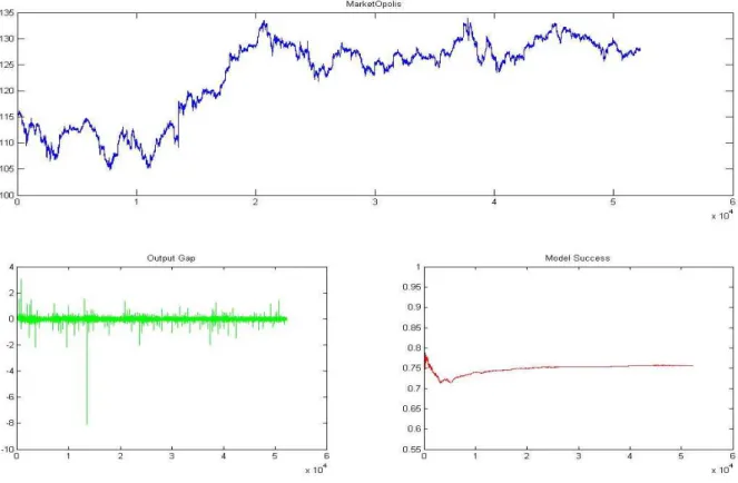
Figure 2 - Summary Stage 1 (without Optimization): Top Chart: Prices derived from the model; Left chart: Output Gap = Hypothetical Price – Real Price; Right Chart: Cumulative success of the model (how many minute can the model predict based on investment decision);
It is relevant to add to the discussion how the weights or investors’ market share changed through the optimization. In order to replicate Apple’s stock price, Market Makers, responsible for 15%, needed to be, on average, 25.11%, Tracker changed from 30% to 21.76%, Mutual Fund from 20% to 15.34%, Fundamental Investor from 10% to 10.15%, Momentum Investor from 10% to 6.64%, Speculator from 5% to 7.49% and Noise Traders from 10% to 13.5%46.
Nevertheless, it must not be forgotten that those results are in-sample, carrying pitfalls and some additional remarks. It is also fundamental to review the overall volume traded and who is behind it. Following Shorter and Miller (2014) studies and within the recent SEC47 realeases, Dark pools48 account for about 15% of the trading volume. Since “Orders sent to dark pools to buy
46 All the values presented are averages of the variable market shares. 47 Security and Exchange Commission
48“A dark pool is a type of alternative trading system (ATS), a broker-dealer who matches the stock trading
[25]
or sell certain stocks are not publicly displayed”49, it is becoming harder to track who is in the market at any given minute. So, any market share or weight proxy of traded volume is as unrealistic and doubtful as the present one. Secondly, the optimization is assuming that there are no more investor profiles and styles out there, rather than those who were described. Thirdly, as a result of the parameters’ optimizing, the model does not have enough robustness to “survive” any fundamental changes in the future. Finally, and despite the success on predicting
Apple’s stock prices, this procedure would have not been possible if the real security prices were not known before, being a pointless method to predict stock prices. Still, a positive link with past weights was found, which is in line with the general consensus that market shares do not change dramatically over a course of one day, on average. By combining those empirical results, this preposition strengths the predictability hypothesis, even though it is not sufficient to put in question the predictability or the ability of consistent higher risk-adjusted earnings.
5 - Conclusions:
As this model demonstrates, while it is known what are the common drivers of the main investors, the ability to predict how the price will react to the aggregate investment decision of all market players is not straightforward. Evidence was found that some players tend to enter in the market when prices show some known characteristics (bullish trends for momentum traders, big drops in prices for fundamental investors, etc.). Having said that, even though we may find some indication of price predictability based on investor decisions, it is premature to state that markets are not efficient and a smart investor can earn consistent risk-adjusted profits above the overall market return.
Besides, as the results previously shown, the output gap between the model and reality is amplified when big movements in stock prices happened. This outcome may be further proof
[26]
that modeling stock market behavior needs to be complemented with variables that control for external changes and events (like earnings announcements, economic releases, net position of the main investors) and a more detailed effect of the co-movement of US stocks to other important World indices.
In order for the present study to be complemented, further studies in this area need to be done. Modifications such as the introduction of tick data (instead of minute data) can be crucial to the accuracy of the model, by adding high-frequency investors. Just as relevant as the addition of more data and more investors, is the introduction of reaction functions when news come out (such as earnings or changes to interest rate or exchange rate). By doing so, it would be possible to gain a deeper knowledge on the investors’ investment decision process.
Finally, it is unquestionable that multiple behavioral biases that interfere with “rational” decisions exist, as shown by several academic studies. Therefore, by not taking these features into account, the model here presented is biased by the insertion of quasi-rational investors with neither price nor time-dependence investment trigger. This can absolutely be questionable, as discussed with financial professionals or academic researchers.
6 - Appendix:
[27] 7 - References
BALVERS, R., WU, Y., & GILLILAND, E. ( 2000). Mean Reversion across National Stock Markets and Parametric Contrarian Investment Strategies. THE JOURNAL OF FINANCE • VOL. LV, NO. 2.
Bernanke, B. S., & Kuttner, K. N. (2003). What Explains the Stock Market’s Reaction to
Federal Reserve Policy? Staff Report, Federal Reserve Bank of New York, No. 174.
Bloomfield, R., O’Hara, M., & Saar, G. (2002). The “Make or Take” Decision in an Electronic
Market: Evidence on the Evolution of Liquidity.
Bodie, Z., Kane, A., & Marcus, A. J. (2011). Investments 9th Edition. McGraw-Hill Irwin.
Bont, W. F., & Thaler, R. (1985). Does the Stock Market Overreact? THE JOURNAL OF FINANCE VOL. XL, NO. 3.
Chaboud, A., Benjamin, C., Hjalmarsson, E., & Vega, c. (2012). Rise of the Machines: Algorithmic Trading In the Foreign Exchange Market.
Chan, L. K., Chen, H.-L., & Lakonishok, J. (2002). On Mutual Fund Investment Styles. The Review of Financial Studies Winter 2002 Vol. 15, pp 1407-1437.
Daniel, K., Hirshleifer, D., & Subrahmanyam, A. (1998). Investor Psychology and Security Market Under- and Overreactions. The Journal of Finance. Vol LIII, No. 6.
De Long, J. B., Shileifer, A., Summers, L., & Waldmann, R. J. (1990). Positive Feedback Investment Strategies and Destabilizing Rational Speculation. The journal of Finance Vol XLV, Nº2.
[28]
De Long, J. B., Summers, L. H., & Waldmann, R. J. (1990). Noise Trader Risk in Financial Markets. Journal of Political Economy, Vol. 98, No. 4, 703-738.
Fama, E. F. (1998). Market effciency, long-term returns, and behavioral finance. Journal of Financial Economics 49 (1998) 283Ð306.
Forbes, K. J., & Rigobon, R. (2001). No Contagion, Only Interdependence: Measuring Stock Market Co-Movements.
Grinblatt, M., Titman, S., & Wermers, R. (1995). Momentum Investment Strategies, Portfolio Performance, and Herding: A study of Mutual Fund Behavior. the American Economic Review, Volume 85, Issue 5 (Dec., 1995), 1088-1105.
Jensen, M. C. (1978). Some Anomalous Evidence Regarding Market Efficiency. Journal Of Financial Economics, Vol. 6, Nos. 2/3 (1978) 95-101.
Kirilenko, A., Kyle, A. S., Samadi, M., & Tuzum, T. (2011). The Flash Crash: The Impact of High Frequency Trading on an Electronic Market.
Lo, A. W. (2004). The Adaptive Markets Hypothesis: Market Effciency from an Evolutionary Perspective.
Madhavan, A. (2011). Exchange-Traded Funds, Market Structure and the Flash Crash.
Malkiel, B. G. (2003). Passive Investment Strategies and Efficient Markets. European Financial Management, Vol 9, No. 1.
Malkiel, B. G. (2003). The Efficient Market Hypothesis and Its Critics. CEPS Working Paper No. 91.
Mutual Funds and the U.S. Equity Market. (December 2000). Federal Reserve Bulletin, 804, 805.