http://dx.doi.org/10.1590/0104-530X2482-15
Resumo: O cálculo do Imposto sobre a Propriedade Predial e Territorial Urbana (IPTU) tem como base o valor venal do imóvel, geralmente estabelecido na planta de valores genéricos (PVG) dos municípios. No entanto, existem municípios, principalmente os de pequeno porte, que não realizam a cobrança do IPTU. Esse fato se deve à desatualização do cadastro imobiliário e à falta de metodologia robusta e fácil para determinação do valor venal,
de pessoal capacitado e de recursos inanceiros. Nesse sentido, o objetivo deste trabalho foi aplicar a combinação
do modelo de regressão espacial e a modelagem dos fatores de localização para determinar o valor venal de cada imóvel de um município de pequeno porte para a geração da planta de valores genéricos. O estudo foi desenvolvido na cidade de São Gotardo/MG. Foram utilizadas 184 amostras de avaliações de imóveis residenciais realizadas
pela Caixa Econômica Federal no período de 2012 a 2013. A im de analisar a aplicação dos modelos espaciais,
foram gerados quatro modelos de regressão múltipla a partir das variáveis dependentes logaritmo do valor total e
logaritmo do valor unitário e das variáveis independentes relativas às características construtivas das ediicações,
conforme estudos anteriores, bem como foram testadas variáveis adicionais referentes às características do terreno. Para os modelos que apresentaram dependência espacial no erro, foi gerado o modelo espacial do erro para
determinar uma nova variável homogeneizada que englobasse o fator localização, (VH), a qual foi utilizada como variável independente de um novo modelo de regressão linear. A escolha do melhor modelo de regressão se deu a partir da análise do menor Coeiciente de Dispersão, bem como pelo atendimento aos pressupostos do modelo de regressão linear. O modelo com a variável dependente logaritmo do valor unitário e a variável homogeneizada como Abstract: The calculation of the Tax on Land and Urban Property (IPTU) is based on property market value, usually established in the city plant of general values (PVG). However, there are municipalities, especially small ones that do not collect IPTU taxes. This is due to outdated real state register, in addition to the lack of qualiied personnel, inancial resources and robust and easy methodology to determine real state market value. Therefore, this work aims to combine the spatial regression model and location factor modeling to determine the market value of each property in a small city for the generation of the table of general values (PVG). The study was conducted in the city of São Gotardo/MG. One hundred and eighty-four samples of residential real state assessments made by Caixa Econômica Federal in 2012 and 2013 were used. Aiming to analyze the application of spatial models, four multiple regression models were generated based on the logarithm dependent variables on the total and unit values, and the independent variables related to the construction characteristics of the constructions, according to previous studies. Additional variables related to the land characteristics were also tested. For the models with spatial error dependence, a spatial error model was generated to determine a new homogenized variable encompassing the location factor (VH), which was used as an independent variable on a new linear regression model. The best regression model was selected based on the compliance of assumptions of the linear regression model and the analysis of the lowest Dispersion Coeficient. The model with the logarithm dependent variable on the unit values and the homogenized variable as independent, showed the best results and observed all the assumptions. Thus, it was demonstrated that the homogenized variable improves the performance of the linear regression model, since it includes the property location factor in the independent variables.
Keywords: Property market value; Small towns; Spatial model; IPTU; Table of general values.
Statistical models for generation of generic values
plants in urban areas
Modelos estatísticos para geração de plantas de valores genéricos em áreas urbanas
Reynaldo Furtado Faria Filho1 Jorge Luís Silva Brito2 Rosiane Maria Lima Gonçalves1
1 Universidade Federal de Viçosa – UFV, Campus de Rio Paranaíba – CRP, Rodovia MG-230, Km 7, CEP 38810-000, Rio Paranaíba,
MG, Brazil, e-mail: [email protected]; [email protected]
2 Universidade Federal de Uberlândia – UFU, Av. João Naves de Ávila, 2121, Bairro Santa Mônica, CEP 38400-902, Uberlândia, MG,
Brazil, e-mail: [email protected]
Received July 16, 2015 - Accepted June 30, 2016
1 Introduction
The growing social demands from the urban development, and the lack of tax resources have demanded from public administrations a big effort
to keep inancial balance between expenditure and
revenues of Brazilian municipalities (Freire et al., 2006).
The tax revenues of the municipalities are taxes, duty and contribution for improvement, whose competency is constitutionally attributed to the local sphere of government. The integral collection for municipalities which institute them are: Services Tax (ISS), Tax on the Emission of Immobile Goods (ITBI), and The Urban Building and Land Tax (IPTU) (Brasil, 2013).
Each municipality organizes its own collection system with a tax code itself, but respecting the rules presented in the Constitution and in the National Tax Code (CTN). The ISS incurs on provision of services to third parties; the ITBI, on transactions involving transfer on the ownership to real state; and the IPTU, on the property owners located in urban area of the city (Brasil, 2013).
The Federal Constitution of 1988 determines IPTU has to be of municipal competence. The calculation of this tax is based on the nominal value of the property, which has to correspond to the sales cash value, being determined by sum of value of the land and construction (Afonso et al., 2010). According to Florencio (2010), the criteria for determining the nominal value of each property of the municipality are established by Plants of Generic Values (PVG).
From 2000, the municipalities had to start an adaptation process which refers to the way of charging IPTU. For several years, this tax was neglected by some public administrators. However, from the Law Fiscal Responsibility, mayors felt it was their obligation to update urban real state registers as well as charge IPTU correctly, under penalty of foregoing income, according to Supplementary Law number 101, of 05/04/2000 (Brasil, 2000).
Mainly small municipalties − population under 50.000 inhabitants (IBGE, 2014a), faced dificulties
to charge IPTU due to out-of-date real state cadastre, and lack of solid methodology and easy use of determining the nominal value of urban properties,
as well as qualiied people and inancial resource.
As the calculation basis of IPTU is the nominal value of the properties, the municipal administration
must always determine it as the most realistic possible way, making this value the closest to the market. However, due to the complexity for determining it, as well as high number of properties to be assessed, it becomes a very hard task (Carvalho, 2011).
According to Afonso et al. (2010), most of Brazilian real state valuations are based on old parameters, and do not take into consideration dynamics impacts that cause impact on valorizing the properties, threatening the collection of IPTU. Besides this, it is the fact of the valuations be highly conditioned to issues of political nature. According to Carvalho (2006, p. 23), “[...] many municipalities use the same land to determine area of the city or even for urban
perimeter, generating signiicant distortions in the
level of the valuations”.
For Florencio (2010), most part of the plants of generic value in the Brazilian municipalities are
outdated or updated based on inlation indices, which
is correct, because the city has no appreciation or devaluation the same way everywhere. This author reports some aspects that explain the distortions in the calculation of Plants of Generic Values (PVG):
• The dificulty of quantifying and qualifying
the several attributes (physical, locational and
economical characteristics) that deine the value
of the property.
• The use of Linear Regression models, which need to take into consideration some basic presumptions as true, which are not always work for the property market.
Another factor to be highlighted is that in many cases, the estimates of property values have as level
of accurancy the veriication of prompt type, which
is an assessment done subjectively, not using any mathematical-statistical procedure (Braulio, 2005); many of these estimates are realized from personal experience or opinion.
According to information from IBGE (2014b), in 2012, the collection of IPTU in Brazil was around R$ 107.40 per inhabitant. The highest collections of IPTU per inhabitant were of R$ 251.60, R$ 154.90 and R$ 126.60, in the states of São Paulo, Rio de Janeiro and Mato Grosso do Sul, respectively. On the other hand, the lowest value was in the state of Maranhão, with only R$ 9.80 per inhabitant. Therefore, it is clear the discrepancy of collection in the Brazilian states.
independente foi o que apresentou melhor resultado, atendendo a todos pressupostos. Dessa forma, foi possível veriicar que a variável homogeneizada melhora a performance do modelo de regressão linear, visto que insere o
fator localização dos imóveis nas variáveis independentes.
An alternative for better determining PVG is the use of a mass evaluation, once in the calculation of a property value, the constructive values might be taken into consideration, being the valuation of property as a result of its location, accessibility, infra-structure (garbage collection, sewage, pavimentation, public lighting, etc.), proximity of hospitals, parks, shopping centers among others (Medvedchikoff, 2009). Silva
& Verdinelli (2000) deine mass evaluation consists
of “ determining values for all properties located in a certain perimeter, by using assessment procedures that should be legally supported”.
Methodologically, what highlights to determine the comercial value of the properties to generate PVG is a mass assessment through the use of techniques that apply spatial econometrics. Trivelloni (2005), using spatial econometrics with analysis and modeling of the factors for location of the properties, obtained the value of average m2 of each square aspect of the
study area, generating PVG.
There is no consense in the literature in relation to the best methodology for determining the commercial value of the property in a mass assessment, mainly for small counties, once works related to small counties were not found in the literauture.
These small municipalities are the ones that need information and techniques the most, which get adjusted to the reality in relation to the assessment of properties, since it is sometimes on them IPTU is not even charged, missing out resources that could be used for the society in a better way of provision of services.
Thus, this study aimed to apply the combination of spatial regression model and modeling of the location factors to determine the commercial value of each property in an urban town for generating of the plant of generic values.
2 Areas, materials and methods
2.1 Study area
The study was carried out in the city of São Gotardo/MG, which is located in the mesoregion of the Triangle Mineiro/Alto Paranaíba. The municipality has an area of approximately 866.087 km2, demographic
density of 36.74 hab./km2, and has as surrounding
municipalities Matutina, Campos Altos, Quartel Geral, Rio Paranaíba, Tiros, Santa Rosa da Serra, Serra da Saudade and Estrela do Indaiá. The urban area of São Gotardo has approximately 5.35 km2,
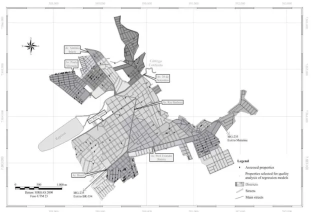
and perimeter of 16.208 m. In Figure 1, the location map of the municipality of São Gotardo is shown.
The growth of the population in the last decades
was signiicant, once the population in 1991 was of
19.697 inhabitants, going up to 31.807 inhabitants in 2010. In relation to the urban population, there
were 16.520 inhabitants in 1991, and in 2010 there were 30.050 inhabitants (IBGE, 2014a).
The main activity of the county is the agricultural production, which was leveraged from 1970 with the implementation of Directed Settlement Program of Alto Paranaíba (PADAP). In relation to technology, the crops (wheat, carrots, potato and garlic) of São Gotardo are among the most developed ones in the country.
The collection of IPTU in São Gotardo, in 2012, was of R$ 562.383.32 (FINBRA, 2014). Thus, in 2012 the collection of IPTU per person in this municipality was of R$ 17.68.
2.2 Materials and methods
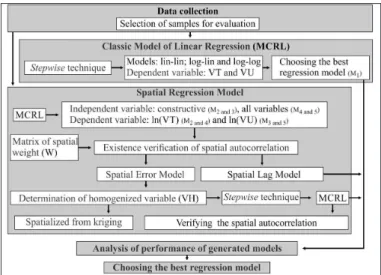
Below, the methodology developed in this work will be described in details. A summary can be seen
in the low chart shown in Figure 2.
2.2.1 Database
The cartographic basis of the city was obtained in the City Hall of São Gotardo. This basis has the road, division per district and some lots.
The assessment of properties was used by Caixa Econômica Federal from 2012 and 2013, in the city of São Gotardo/MG. All loan processes were made available for consultation in this period. One of the contents of these processes are the valuation reports, which were scanned for use in this research. After tabulating all information in an Excel sheet and verifying its inconsistency, 184 assessed properties remained, which were used for the development of this work. All information refers to residential properties.
Having the address of the properties assessed, the situation of each one was registered with the recipient GPS Garmin GPSMAP 78s. Each point referring to assessed properties was inserted (from UTM coordinates) in the cartographic basis available by the City Hall of São Gotardo.
2.2.2 Available variables
The available variables in the valuation report provided by Caixa were divided into four categories: price of the property; characteristics of the land; constructive characteristics of the construction; and characteristics of valuation. In Table 1 a summary of the characteristics for all available variables is presented. The acronyms, descriptions and units of each unit are also inserted in it.
Beron et al., 2004). Thus, an older propriety would get a compensation for this possible remodeling made.
2.2.3 Selection of samples for quality analysis of regression models
For realizing the quality analysis of prediction for the value of the property, 10% of 184 assessed properties was approximately selected by Caixa from 2012/2013. Initially the standardization of all variables was done by its standard-deviation, in other words: (variable value average /standard-deviation .− ) Later,
the nonhierarchical grouping analysis was carried out (K-means), through the module Spatial Statistics
Tools of ArcGIS software, in which no 184 properties
were divided into ive groups.
From the grouping result, it was possible to identify which samples were similar. After that, a selection of approximately 10% of the samples of each group was randomly done through the module Geostatistical Analyst Tools of ArcGIS software.
Therefore, all analyses done during the work were based on the 166 samples of the properties. In Figure 3, a location map with each sampling point and the points selected for the quality analysis of the regression models generated is shown. It is possible to observe the 18 samples selected for quality analysis of the models are randomly displaced in the area studied.
Figure 2. Flow chart with the procedures adopted in the work. Note: M1, M2, M3... are the regression models generated.
Table 1. Available variables in the assessment of properties of Caixa.
Category Variable Acronym Description/deinition of the variable Unit
Price of the property
Total value of the property VT Total value of the property assessed Real Unit value of the property VU Total value of the property assessed / built-up area Real/m2
Characteristics of the land
Form of the land FO Irregular or Triangular = 0
Rectangular or Trapezoidal = 1
-Share/Greide of the land CT1, CT2
If CT1 = 0; CT2 = 0: Under the street level If CT1 = 1; CT2 = 0: Above the street level If CT1 = 0; CT2 = 1: In the street level
-Inclination of the land IT1, IT2
If IT1 = 0; IT2 = 0: Bumpy
If IT1 = 1; IT2 = 0: Uphill/Slope > 10%
If IT1 = 0; IT2 = 1: Flat/semilat
-Area of the land AT Total area of the land of the valuated land (m2)
Front of the land FT Measurement of the front land (m)
Situation of the land ST
Placement of the land in relation to the square: mid block = 0
corner = 1
-Constructive characteristics of construction
Number of loor NP
Number of loor of the construction 1 loor = 0
2 or 3 loors = 1
-Age ID Age of the construction (years)
Age2 ID2 Age of the construction squared (year)2
Standard of inishing PA1, PA2,
PA3
If PA1, PA2, PA3 = 0: Minimum or between low and minimum
If PA1 = 1; PA2, PA3 = 0: Low or Between normal and low
If PA2 = 1; PA1, PA3 = 0: Normal or Between normal and high
If PA3 = 1; PA1, PA2 = 0: High
-State of conservation of
the property EC1, EC2
If EC1 = 0; EC2 = 0: Bad If EC1 = 1; EC2 = 0: Regular If EC1 = 0; EC2 = 1: Good
-Garage GA There is no garage = 0
There is a garage = 1
-Constructed area AC Total constructed area of the assessed property (m2)
Number of Rooms/Suites NQ Total number of rooms and/or suítes of the assessed
property
-Number of Bathrooms NB Total number of bathrooms in the assessed property
-Characteristics
of assessment Assessment Date DA
Year of assessment of the property 2012 = 0
2013 = 1
-2.2.4 Classic Model of Linear Regression (MCRL)
For Gujarati (2000, p. 185), the equation of MCRL “[...] provides the average or the expected value of
conditional Y to the ixed values (in repeated sampling)
of X1, X2,..., Xk”. In general, MCRL can be written as shown in the Equation 1:
0 1 1 2 2 ki 1, 2, 3, ,
i i i k i
Y =β +βX +β X +…+β X +µ i= …n (1)
in which: Yi: dependent variable; X aX1i ki: k-1 explanatory
variables; β0: intercept; β β1a k: partial coeficient of
inclination; µ: error; i: i-ith observation; and n: size of the sample.
The stepwise technique was applied, which aims to group the independent variables that represent the best way of regression model. For this, the SPSS software was used in order to obtain a regression model only with relevant variables automatically. As parameters for this method, the probability of test F lower than 5%, and the exclusion higher
than 10% of signiicance was used for inclusion
of a variable.
To verify the best arrangement between dependent and independent variables, the following regression models were used: linear (lin-lin), semilog (log-lin) and logarithmic (log-log). For this, the total value
(VT) and unit value (VU) of the properties were used as dependent variables.
The use of VT and VU variables as dependent
is justiied due to the fact there is no unanimity in
the literature consulted. Of the 33 consulted works, referring to the generation of some econometric model related to the value of the property, 10 of them used the unit value as dependent variable, in other words, the total value of the property divided by the constructed area (Brondino, 1999; Carvalho, 2011; Florencio, 2010; Gomes et al., 2012; Hochheim & Uberti, 2001; Michael, 2004; Pelli, 2006; Ribeiro, 2011; Trivelloni, 2005; Vazquez, 2011); 19 works used the total value of the property as dependent variable (Araújo et al., 2012; Avila, 2010; Braulio, 2005; Coelho, 2007; Dalaqua, 2007; Dantas, 2003; Dubin, 1992; Furtado, 2011; Gazola, 2002; Koschinsky et al., 2012; Matta, 2007; McCluskey et al., 1997; Monteiro & Leite, 2011; Moura & Carneiro, 2004; Paixão, 2010; Sander & Haight, 2012; Schiavo & Azevedo, 2003; Sousa & Arraes, 2005; Vieira, 2005); and four works used the total and unit values, separately, as dependent variables (Anselin & Lozano-Gracia, 2008; Catalão, 2010; González, 2002; Marques et al., 2009).
Finally, the normality tests, heterocedasticity and multicolinearity of all regression models generated were done.
2.2.5 Spatial Regression Model
Four models of multiple regression were generated from the dependent variables Ln(VT) and Ln(VU). For this, initially, only the constructive characteristics of the constructions, and after that, all available variables were used as independent variables. Thus, four combinations of linear regression models were generated to know: M2 (Ln(VT) as dependent variables and constructive variables as independent ones), M3 (Ln(VU) as dependent variable and constructive variables as independent ones), M4 (Ln(VT) as dependent variable and all available variables as independent ones) and M5 (Ln(VU) as dependent variable and all available variables as independent ones).
After that, the matrix of spatial weights (W) was generated through GeoDaSpace software.
The deinition for the value of maximum distance so
that two properties were considered neighbors was realized from the achievement value semivariogram of the homogenized variable (which represents the factor of location). This value was of approximately 1.350 m, which is not the reality for the studied area. Thus, this value was being reduced up to getting to 800 m, whichs represents in a more accurate way the property reality of São Gotardo. Therefore, the matrix of spatial weight was determined using the geographic distance, in which the properties up to the cutting distance (800 m) are considered neighbors and receive the unit value (1), and from the cutting distance are not considered neighbors, receiving value zero. This matrix was standardized by sum of the line.
Using the models M2, M3, M4, M5 and the spatial
matrix of weights, the existence veriication of spatial
autocorrelation through Robust Lagrange Multiplier test (LM) of spatial lag and error. In order to analyze the application of all possible models, when LM test
indicated signiicance in the spatial lag and in the
error, two models were generated, differently from the one that is usual in the studied literature, which
uses only what is signiicant.
Anselin (1988) developed the methodology that uses econometric techniques for studying the existence of spatial dependence. This dependence occurs when the observations of an i local depend on other observations located in other places j, given that i ≠ j, can be modeled in two ways:
• Spatial Lag Model or SAR (Spatial Autoregressive Model): in case of value of properties, this occurs
when the value of a property is inluenced by the
value of transactions realized in the neighborhood. The Equation 2 presents the spatial lag model:
WY
Y=Xβ ρ+ +ε (2)
in which: Y: dependent variable; X: independent
variables; β: parameters of the model; ρ: coeficient
of spatial autocorrelation that represents the average
inluence of the neighboring unit; W: spatial matrix of weights that links the variables in different locals;
and ε: residues of the model.
• Spatial Error Model or SEM (Spatial Error
Model): occurs when the error term of a local
is correlated with the error values of other neighboring places. In the Equation 3, the spatial error model is presented:
Y=Xβ λ ε+ W +u (3)
in which: Y: dependent variable; X: independent
variables; β: parameters of the model; λ: coeficient of
spatial autocorrelation; W: spatial matrix of weights
that links the variables in different locals; ε: residues
of the model; and u: non-correlated residues. When generating the spatial error model, it was aimed to determine a new homogenized model that involved the location factor. For this, the methodology recommended by Trivelloni (2005) was used, in which the new homogenized value (VH) of each sample was determined from the division of VT or VU by the spatial error model without its constant
and λ (lambda).
This new homogenized variable, which represents the location factor, was used as independent variable of a new linear regression model (MQO). This model was generated using the stepwise technique. Later on,
a new veriication of spatial autocorrelation existence
through Robust Lagrange Multiplier tests (LM) of spatial lag and error.
In relation to the determination of homogenized variable (VH), for any property present in the studied area, an interpolation of this one was done using kriging.
2.2.6 Analysis of performance of generated models
To analyze the performance of regression models generated, the methodology recommended was applied
by the International Association of Assessing Oficers
(IAAO). This association says the measurement of variability or uniformity of an assessment has to be
carried out through the Coeficient of Dispersion
(COD) (IAAO, 2013). Thus, the determination of COD was done as described in Equation 4:
average median COD *100 median c c o o c o P P P P P P − = (4)
in which: COD: coeficient of dispersion; Pc: estimated
according to IAAO (2013), the value of acceptable COD goes up to 15.
2.2.7 Practical analysis of inal regression
model
For Gazola (2002), the fact of the model meet the assumptions is not guarantee of quality for predictions, being a practical assessment necessary, which shows if in fact there is quality of adjustement and predictive capacity. Thus, the percentage of error can be determined by (Equation 5):
( ) abs MappedValueObserved( MapedValueEstimated)
Error % *100
MappedValueObserved
−
= (5)
Values of error up to 5% are considered an excellent result; between 5 and 10%, very good result between 10 and 15%, good result; and between 15 and 20%, acceptable result (Gazola, 2002).
To realize a spatial error analysis of prediction in m2 values of constructed area of São Gotardo, two
maps were generated through the application of kriging as: the map of m2 values of assessed construction
by CEF; and m2 values of construction estimated
by M7 regression model for the 184 properties used in this study.
After that, the algebra of these two maps was done, aiming to determine the locals with higher and lower successes through Equation 6:
( ) abs MappedValueObserved( MapedValueEstimated)
Error % *100
MappedValueObserved
−
= (6)
3 Results and Discussion
3.1 Classic Model of Linear Regression (MCRL)
Three regression models were generated for the dependent variable VT (lin-lin, log-lin and log-log), using the stepwise technique and SPSS software.
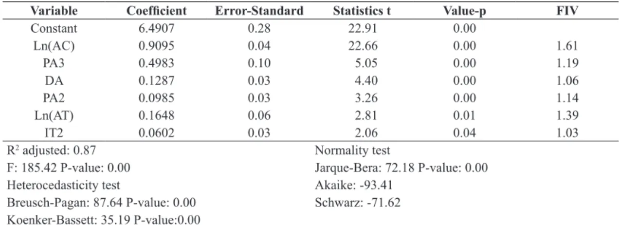
In Table 2, the model with better result in relation to paramenters R2 is shown, adjusted and statistics
of Akaike and Schwarz. This model, here called M1, showed higher value of R2 adjusted (0.87), and lower
value of Akaike and Schwarz, in comparation to the other models tested.
M1 model has as dependent variable the logarithm of total value of properties and logarithm of independent variables, except the dichotomous ones. In Table 2, it is possible to observe the variables inclination of
the lat land/semi-lat (IT2), and logarithm of the land area (Ln(AT)) were signiicant at 5%, while
the logarithm of constructed area (Ln(AC)), the high
inishing standard (PA3), the validation date (DA) and the regular inishing standard or between regular and high (PA2) were signiicant at 1%.
In relation to MCRL assumptions, M1 model did not meet the assumptions of normality and homocedasticity, once the tests of Jarque-Bera, Breusch-Pagan and
Koenker-Bassett were signiicant. According to
Gujarati (2000), the values of Factor of Variance
Inlation (FIV) lower than 10, have an acceptable
level of correlation and do not cause damage to the model. Thus, for M1 model, it is veriied the effect
of multicolinearity is not signiicant.
Three other regression models were generated with dependent variable unit value (VU); however, R2 adjusted varied from 0.25 to 0.21. Thus, due to
its low performance, these models are not shown in this work.
3.2 Spatial regression model
The models that used spatial regression techniques were generated independently of the models estimated by MCRL, permitting to analyze the diferences and/ or similarities between the methods.
Four MCRL were generated, having as dependent variables the total and unit values of the properties,
Table 2. Regression Model (M1) log-log referring to the dependent variable logarithm of the total value of the properties (VT).
Variable Coeficient Error-Standard Statistics t Value-p FIV
Constant 6.4907 0.28 22.91 0.00
Ln(AC) 0.9095 0.04 22.66 0.00 1.61
PA3 0.4983 0.10 5.05 0.00 1.19
DA 0.1287 0.03 4.40 0.00 1.06
PA2 0.0985 0.03 3.26 0.00 1.14
Ln(AT) 0.1648 0.06 2.81 0.01 1.39
IT2 0.0602 0.03 2.06 0.04 1.03
R2 adjusted: 0.87 Normality test
F: 185.42 P-value: 0.00 Jarque-Bera: 72.18 P-value: 0.00
Heterocedasticity test Akaike: -93.41
Breusch-Pagan: 87.64 P-value: 0.00 Schwarz: -71.62 Koenker-Bassett: 35.19 P-value:0.00
and as independent ones, only the constructive variables (following the methodology suggested by Trivelloni, 2005), and with all variables available as independent ones to analyze if the model improves the quality when there are more variables involved.
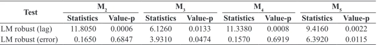
After that, the matrix of spatial weights was generated, using as cutting distance, so that the two properties were considered neighbors the value of 800 m. In order to verify the existence of spatial autocorrelation, Robust Lagrange Multiplier tests of error and spatial lag were realized, using the matrix of spatial weights generated. The results of these tests are presented in Table 3.
From this table, it is possible to verify that (M2) model generated with dependent variable logarithm of total value Ln(VT) of the properties and with
constructive variables as independent signiicant effect
at 1% only in the spatial lag. For (M3) model, in which the independent variables of M2 were maintained (constructive variables), and using as independent variable the logarithm of unit value Ln(VU), the existence of autocorrelations in spatial lag and error
was veriied, being these signiicant at 5%.
Yet, from Table 3, it is observed (M4) model, which has as dependent variable the logarithm total value of the properties and with all independent available
variables, was identiied signiicant effect at 1% only
in spatial lag. Finally, for (M5) model with dependent variable logarithm of unit value of properties and as independent variables all the available ones, it was possible to observe the existence of autocorrelation in
spatial lag and in error, being signiicant at 1 and 5%,
respectively.
When conirmed the autocorrelation in spatial lag
and/or error, the following models of spatial lag and/or error model were generated. Due to high number of models generated, two models that presented the best result will be shown in the following topics. The two best models (M3 and M5) were generated with dependent variable logarithm of unit value of
the properties. Both models presented signiicant
effect in spatial lag; however, when generated the model of spatial lag, the results were not good, once they did not show the variable constructed
area (AC) as signiicant, and yet, the value of R2
adjusted was low.
3.2.1 Model with dependent variable ln(VU) and constructive variables of constructions as independent (M3)
As M3 model showed the spatial autocorrelation in the residues, the suggested methodology was applied by Trivelloni (2005), in which a homogenized variable referring to the property location. Thus, iinitially the spatial error model was generated through GeoDaSpace software. The result of this model is shown in Equation 7:
Ln(VU) = 6.9512 - 7.24E-05 * AC + 0.2098 * EC1 + 0.2071 * EC2 - 0.0536 * GA - 0.0102 * ID + 0.0004 * ID2 + 0.0291 * NB - 0.0533 * NP - 0.0381 * NQ + 0.0603 * PA1 + 0.1351 * PA2 + 0.4799 * PA3 + 0.3524 * LAMBDA
(7)
The homogenized unit value (VHU) for each property was determined by (Equation 8):
VHU = VU / exp(- 7.24E-05 * AC + 0.2098 * EC1 + 0.2071 * EC2 - 0.0536 * GA - 0.0102 * ID + 0.0004 * ID2 + 0.0291 * NB - 0.0533 * NP - 0.0381 * NQ + 0.0603 * PA1 + 0.1351 * PA2 + 0.4799 * PA3)
(8)
With the value of VHU calculated for each property, it was possible to generate a new model MQO with this variable. This model guarantees the spatial
effects that inluenced the M3 model negatively,
and are not present anymore because the effects are inserted in the variable VHU. Thus, M6 model with independent variable VHU is presented in Table 4. It is highlighted the dependent variable used was Ln(VU), and the stepwise technique was applied by SPSS software. It is also observed in Table 4 that all
variables presented were siginiicant at 1%, except the standard variable of low inishing or between regular or low (PA1), which was signiicant at 5%.
The value of R2 adjusted was of 98%.
In relation to MCRL assumptions, M6 model did not meet normality (test of Jarque-Bera) and homocedasticity for the test of Breusch-Pagan,
although it was presented non-signiicant at 1% for
heterocedasticity for the test of Koenker-Bassett. In relation to the FIV of multicolinearity, the variables EC2, PA1 and PA2 presented values higher than 10, which demonstrates the multicolinearity in them. Thus, the removal of these variables of model,
but the effect of this removal on the signiicance
of other variables was negative, in other words,
Table 3. Tests of spatial autocorrelation.
Test M2 M3 M4 M5
important variables that were signiicant were
not anymore. Therefore, it was chosen to keep all resulting variables of application of stepwise
technique in M6 model.
The test LM robust (lag) presented value-p of 0.8960, and LM robust (error), of 0.2395. Thus, it is possible to verify that there is no spatial autocorrelation in M6 model, which demonstrates the independent variable VHU covers the characteristics of location in the regression model calculated by MQO.
3.2.2 Model with dependent variable ln(VU) and all available variables as independent (M5)
From the conirmation of the existence of spatial
autocorrelation in the residues, although lower the autocorrelation of spatial lag, it was decided to generate the spatial model of error through GeoDaSpace software. The result of this model is shown in Equation 9:
Ln (VU) = 6.9471 - 4.01E-04 * AC + 8.48E-04 * AT + 0.0066 * CT1 - 0.0103 * CT2 + 0.1503 * DA + 0.0930 * EC1 + 0.0513 * EC2 + 0.0177 * FO - 0.0059 * FT - 0.0781 * GA - 0.0199 * ID + 7.91E-04 * ID2 - 0.0241 * IT1 + 0.0292 * IT2 + 0.0326 * NB - 0.0457 * NP - 0.0467 * NQ + 0.0599 * PA1 + 0.1545 * PA2 + 0.5684 * PA3 + 0.0585 * ST + 0.1671 * LAMBDA
(9)
After that, the homogenized unit value (VHU1) was generated for each property through the Equation 10:
VHU1 = VU / exp(- 4.01E-04 * AC + 8.48E-04 * AT + 0.0066 * CT1 - 0.0103 * CT2 + 0.1503 * DA + 0.0930 * EC1 + 0.0513 * EC2 + 0.0177 * FO - 0.0059 * FT - 0.0781 * GA - 0.0199 * ID + 7.91E-04 * ID2 - 0.0241 * IT1 + 0.0292 * IT2 + 0.0326 * NB - 0.0457 * NP - 0.0467 * NQ + 0.0599 * PA1 + 0.1545 * PA2 + 0.5684 * PA3 + 0.0585 * ST)
(10)
The variable VHU1 was used as independent variable in a new multiple regression model generated by MQO. Thus, the guarantee of all location effects not considered in model M5 was aimed, and will be represented by this variable in M7 model.The model (M7) resulting from the application of stepwise
technique is presented in Table 5.
It is observed in model M7 all variables were
signiicant at 1%. R2 adjusted was of 0.81, and
the normality assumptions (test of Jarque-Bera), homocedasticity (Breusch-Pagan, Koenker-Bassett) and multicolinearity were met.
The test LM robust (lag) showed value-p of 0.1473,
and LM robust (error), of 0.5172. Thus, it was veriied
there is no spatial autocorrelation in the model M7, which demonstrates the independent variable VHU1 involves characteristics of location in the regression model calculated by MQO.
3.3 Choosing the best regression model
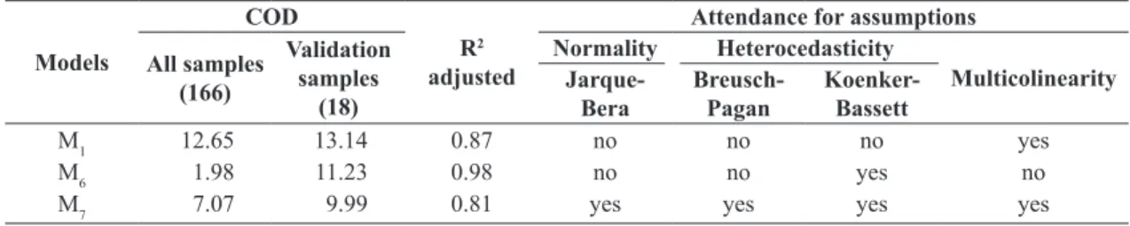
In Table 6, the values of COD are presented and a summary of all assumptions of the models M1, 6 and 7.
The coeficient of dispersion (COD) of all models
met the recommendation of IAAOof a lower value
Table 4. MQO model (M6) with the variable VHU location.
Variable Coeficient Error-Standard Statistics t Value-p FIV
Constant 6.0180 0.03 199.01 0.00
AC -2.16E-04 0.00 -2.71 0.01 3.49
EC1 0.2003 0.02 8.18 0.00 9.46
EC2 0.1932 0.03 7.57 0.00 11.33
GA -0.0494 0.01 -6.76 0.00 1.21
ID -0.0148 0.00 -11.04 0.00 8.87
ID2 5.56E-04 0.00 11.93 0.00 6.23
NB 0.0301 0.00 8.38 0.00 1.94
NP -0.0750 0.01 -7.78 0.00 1.31
NQ -0.0444 0.00 -9.20 0.00 1.48
PA1 0.0391 0.02 2.19 0.03 13.55
PA2 0.1195 0.02 6.37 0.00 14.47
PA3 0.5063 0.03 19.39 0.00 2.75
VHU 9.41E-04 0.00 74.71 0.00 1.02
R2 adjusted: 0.98 Normality test
F: 530.89 P-value: 0.00 Jarque-Bera: 2381.98 P-value: 0.00
Eterocedasticity tests Akaike: -667.83
than 15.0. M6 is highlighted, which presented value of 1.98 for the 166 samples used to generate the regression models. On the other hand, it was observed discrepancy in relation to the value of COD of the 18 samples not used for generating the models, which can indicate some kind of incoherence in this model. Thus, M7 seems to be more trustworthy, once the value of COD for validation samples was the lowest among all the other models.
In relation to R2 adjusted, M
6 present the best result
(0.98), and M7, the worst one (0.81). Finally, it was
veriied that only model M7 met all the assumptions;
therefore, the inal model to be used for determining
the values of properties with the objective of generating the plant of generic values for the urban area of São Gotardo.
3.4 Determination of homogenized variable VHU1 for São Gotardo
The most recommended model for generating the plant of generic values is (Equation 11):
VU = exp(5.9697 - 1.01E-03 * Constructed area + 6.60E-04 * Area of the land - 0.0205 *
Age of the property+ 7.57E-04 * Age of the property2 + 0.0514 * Inclination of the land2 + 0.0310 * Number of Bathrooms + 0.0785 * Standard of inishing2 + 0.4563 * Standard of inishing3 + 9.46E-04 * Homogenized VariableU1)
(11)
Therefore, to evaluate a property in any urban area of São Gotardo using the model M7, it is necessary to obtain the value of the location variable, VHU1. For this, a map of the variable VHU1, was generated, estimated by kriging.
According to Trivelloni (2005), kriging is the most recommended technique to generate the spatialized map of homogenized variable. Thus, initially, four semivariograms of the variable VHU1 were generated, through GS+ software in the directions 0º, 45º, 90º and 135º, in which the negligible difference in the value was noted in the reaching value and level in these directions, proving the isotropy. In Figure 4a,
Table 5. MQO model (M7) with the variable of VHU1 location.
Variable Coeficient Error-Standard Statistics t Value-p FIV
Constant 5.9697 0.05 122.58 0.00
AC -1.01E-03 0.00 -4.95 0.00 2.86
AT 6.60E-04 0.00 5.76 0.00 1.61
ID -0.0205 0.00 -5.96 0.00 7.20
ID2 7.57E-04 0.00 5.69 0.00 6.32
IT2 0.0514 0.01 3.56 0.00 1.03
NB 0.0310 0.01 3.07 0.00 1.90
PA2 0.0785 0.02 5.19 0.00 1.17
PA3 0.4563 0.05 8.93 0.00 1.31
VHU1 9.46E-04 0.00 23.35 0.00 1.01
R2 adjusted: 0.81 Normality test
F: 79.89 P-value: 0.00 Jarque-Bera: 0.51 P-value: 0.77
Heterocedasticity tests Akaike: -325.06
Breusch-Pagan: 7.41 P-value: 0.59 Schwarz: -293.94 Koenker-Bassett: 8.56 P-value: 0.48
Table 6. Values of COD and assumptions of each model generated.
Models
COD
R2
adjusted
Attendance for assumptions
All samples (166)
Validation samples
(18)
Normality Heterocedasticity
Multicolinearity
Jarque-Bera
Breusch-Pagan
Koenker-Bassett
M1 12.65 13.14 0.87 no no no yes
M6 1.98 11.23 0.98 no no yes no
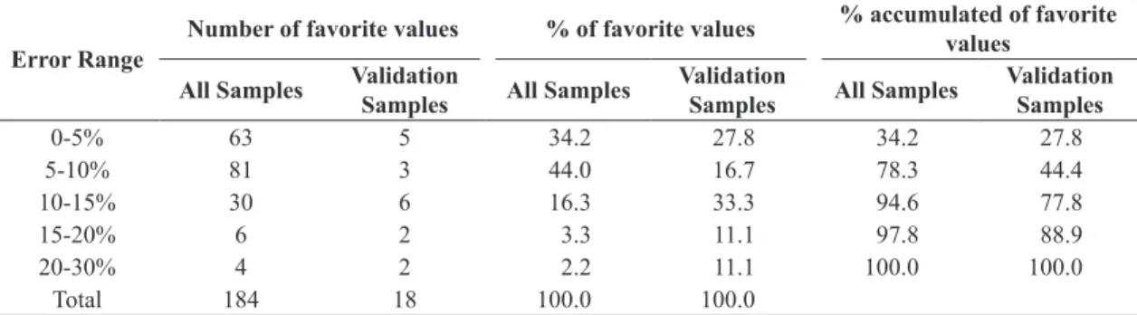
that 70.6% of the validation samples (17 samples) of the predicted values were lower than 15% of error. This study presented 88.9% of the validation samples below the range of acceptable error with the limit up to 20%, which reinforces the quality of its prediction.
For spatial error analysis, two maps were generated through the application of kriging. Figure 5a shows the map of unit values of the assessed properties by CEF, and Figure 5b, the unit values of the properties estimated by M7. It is possible to verify in the range that goes from Centro to the district Jardim das Flores are the most valorized locals. It is also observed the amplitude of the unit value was higher in the estimated map.
The visual analysis of the two maps does not permit to infer major differences between the observed and estimated values Thus, the agebra of the maps was done according to Equation 6.
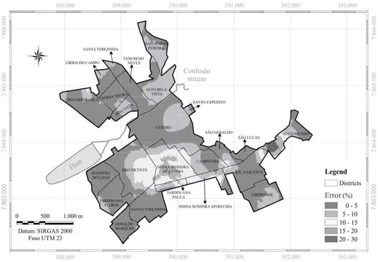
The observed result in Figure 6 shows the districts Nossa Senhora de Fátima and Novo Mundo presented a higher error, demonstrating model M7 should be applied with caution in these districts. This fact was expected because they are areas with lower number of isotropic semivariogram is presented with its all
main characteristics.
In Figure 4b map of spatialized VHU1 is presented from kriging. It is observed in this map the highest values of homogenized values VHU1 are located in
the urban center area of Sāo Gotardo, followed by
the districts Mansões dos Lagos, Jardins das Flores, Campestre and Nossa Senhora de Fátima. This result indicates in these locals the local variable, which
takes the inluence of the neighborhood has more
impact on the unit value of the property.
3.5 Practical assessment of M7 model
In Table 7 the values of error calculated for this work are presented. It is possible to observe in it that when the 184 samples were used, 94.6% of the points presented values of error lower than 15%, while for the 18 validation samples, this value was of 77.8%. Therefore, taking into consideration the parameter, it is possible to say the result of the model was good and can be used for the calculation of property values in
the urban area of São Gotardo. Gazola (2002) veriied
Figure 4. (a) Isotropic semivariogram of the homogenized variable VHU1; (b) map of VHU1 spatialized from kriging.
Table 7. Error for all samples and only for validation samples.
Error Range
Number of favorite values % of favorite values % accumulated of favorite
values
All Samples Validation
Samples All Samples
Validation
Samples All Samples
Validation Samples
0-5% 63 5 34.2 27.8 34.2 27.8
5-10% 81 3 44.0 16.7 78.3 44.4
10-15% 30 6 16.3 33.3 94.6 77.8
15-20% 6 2 3.3 11.1 97.8 88.9
20-30% 4 2 2.2 11.1 100.0 100.0
because 99.3% of the pixels presented acceptable error, in other words, the error value lower than 20%.
4 Conclusion
In view of the results, it was possible to conclude that:
- The inal model can be applied individually for
each property in the municipality studied, being necessary to obtain the variables constructed area, area of the land, age of the property, inclination of the land, number of bathrooms, standard of
inishing and the homogenized variable for
samples, once the district Nossa Senhora de Fátima is old with residential properties that do not go through changes frequently. On the other hand, the district Novo Mundo is new, having no construction. The other districts showed error values lower than 20%, which is considered acceptable according to Gazola (2002).
A counting of pixels was realized for each error range, in which 60.5% of the pixels presented error values lower than 5%; 86.0%, below 10%; 96.1%, below 15%; and 99.3%, below 20%. According to the
classiication of Gazola (2002), this result makes it
possible to say the model can be used in the calculation of property values in the urban area of São Gotardo
Figure 5. (a) Map of unit values assessed by CEF; (b) map of unit values estimated by M7 regression model.
iscal e dá outras providências. Brasília, DF: Diário Oficial da República Federativa do Brasil. Recuperado em 15 de fevereiro de 2013, de http://www.planalto. gov.br/ccivil_03/leis/LCP/Lcp101.htm
Brasil. (2013). O que são os impostos?. Recuperado em 15 de fevereiro de 2013, de http://www.brasil.gov.br/ economia-e-emprego/2010/01/o-que-sao-os-impostos
Braulio, S. N. (2005). Proposta de uma metodologia para a avaliação de imóveis urbanos baseado em métodos estatísticos multivariados (Dissertação de mestrado). Universidade Federal do Paraná, Curitiba.
Brondino, N. C. M.(1999). Estudo da inluência da acessibilidade no valor de lotes urbanos através do uso de redes neurais (Tese de doutorado). Universidade de São Paulo, São Carlos.
Carvalho, P. H. B. (2006). O IPTU no Brasil: progressividade,
arrecadação e aspectos extra-iscais (Texto para Discussão, 1251). Brasília: Ipea.
Carvalho, P. H. B., Jr. (2011). O sistema avaliatório municipal de imóveis e a tributação do IPTU no Rio de Janeiro. (Dissertação de mestrado). Universidade do Estado do Rio, Rio de Janeiro.
Catalão, A. T. M. (2010). Estudo do mercado imobiliário de Aveiro (Dissertação de mestrado). Universidade de Aveiro, Aveiro.
Coelho, M. C. V. (2007). Uso de critérios técnicos para agrupamento de bairros de qualidade de localização similares – cluster. In Anais do XIV Congresso Brasileiro
de Engenharia de Avaliações e Perícias (pp. 1-24). Salvador: IBAPE.
Dalaqua, R. R. (2007). Aplicação de métodos combinados de avaliação imobiliária na elaboração da Planta de Valores Genéricos (Dissertação de mestrado). Faculdade de Ciências e Tecnologia, Universidade Estadual Paulista, Presidente Prudente.
Dantas, R. A. (2003). Modelos Espaciais aplicados ao
mercado habitacional: um estudo de caso para a cidade
do Recife (Tese de doutorado). Universidade Federal de Pernambuco, Recife.
Dubin, R. (1992). Spatial autocorrelation and neighborhood quality. Regional Science and Urban Economics, 22(3), 433-452. http://dx.doi.org/10.1016/0166-0462(92)90038-3.
Finanças do Brasil – FINBRA. (2014). Contas anuais. Recuperado em 20 agosto de 2014, de http://www. tesouro.fazenda.gov.br/pt_PT/contas-anuais
Florencio, L. A. (2010). Engenharia de avaliações com base em modelos GAMLSS (Dissertação de mestrado). Universidade Federal de Pernambuco, Recife.
Freire, A. E., Aguiar, R. O., & Meireles, S. D. (2006). Auditoria da planta de valores pelos Tribunais de
each property belonging to the urban area of the county.
- The inclusion of characteristics of the land improved the estimate of the variable referring to location.
- It was evident the indiscriminate use of classic model of linear regression in this work without considering the location variable can take to wrong estimates of the market value of the properties.
- The dependent variable Total Value showed better results when the classic model of regression was used; on the other hand, when the varible referring to location is inserted, the dependent variable Unit Value became more relevant.
References
Afonso, J. R. R., Araujo, E. A., & Nóbrega, M. A. R. (2010). Um diagnóstico sobre o grau de aproveitamento
do imposto como fonte de inanciamento local (No. 3, pp. 1-48). Cambridge: Lincoln Institute of Land Policy.
Anselin, L. (1988). Spatial econometrics: methods and models. Dordrecht: Kluwer Academic.
Anselin, L., & Lozano-Gracia, N. (2008). Errors in variables and spatial effects in hedonic house price models of ambient air quality. Empirical Economics, 34(1), 5-34. http://dx.doi.org/10.1007/s00181-007-0152-3.
Araújo, E. G., Pereira, J. C., Ximenes, F., Spanhol, C. P., & Garson, S. (2012). Proposta de uma metodologia para a avaliação do preço de venda de imóveis residenciais em Bonito/MS baseado em modelos de regressão linear múltipla. P&D em Engenharia de Produção, v. 10, n. 2, p. 195-207.
Avila, F. M. (2010). Regressão linear múltipla: ferramenta utilizada na determinação do valor de mercado de imóveis (Trabalho de conclusão de curso). Universidade Federal do Rio Grande do Sul, Porto Alegre.
Beron, K. J., Hanson, Y., Murdoch, J. C., & Thayer, M. A. (2004). Hedonic price functions and spatial dependence: implications for the demand for urban air quality. In L. Anselin, R. J. Florax & S. J. Rey (Eds.), Advances in
spatial econometrics: methodology, tools and applications (pp. 267-281). Berlin: Springer-Verlag.
Bourassa, S., Hamelink, F., Hoesli, M., & MacGregor, B. (1999). Defining residential submarkets. Journal
of Housing Economics, 8(2), 160-183. http://dx.doi. org/10.1006/jhec.1999.0246.
Brasil. (2000, 5 de maio). Lei Complementar n°. 101, de
4 de maio de 2000. Estabelece normas de inanças
Contas. In Anais do XI Simpósio Nacional de Auditoria de Obras Públicas (pp. 1-21). Foz do Iguaçu: TCE-PR. Furtado, B. A. (2011). Análise quantílica-espacial de
determinantes de preços de imóveis urbanos com matriz
de bairros: evidências do mercado de Belo Horizonte (Texto para Discussão, 1570). Brasília: IPEA.
Gazola, S. (2002). Construção de um modelo de regressão para avaliação de imóveis (Dissertação de mestrado). Universidade Federal de Santa Catarina, Florianópolis.
Gomes, A. E., Maciel, V. F., & Kuwahara, M. Y. (2012). Determinantes dos preços de imóveis residenciais verticais no município de São Paulo. In Anais do XL Encontro Nacional de Economia (pp. 1-19). Porto de Galinhas: ANPEC.
González, M. A. S. (2002). Aplicação de técnicas de
descobrimento de conhecimento em base de dados e de inteligência artiicial em avaliações de imóveis (Tese de doutorado). Universidade Federal do Rio Grande do Sul, Porto Alegre.
Gujarati, D. N. (2000). Econometria básica (3 ed.). São Paulo: Makron Books.
Hochheim, N., & Uberti, M. S. (2001). Uso de variáveis ambientais na avaliação de imóveis urbanos: uma contribuição à valoração ambiental. In Anais do XI
Congresso Brasileiro de Engenharia de Avaliações e
Perícias (pp. 1-28). Guarapari: IBAPE.
Instituto Brasileiro de Geografia e Estatística – IBGE. (2014a). Cidades. Recuperado em de 13 março de 2014, de http://www.ibge.gov.br/cidadesat/topwindow.htm?1
Instituto Brasileiro de Geografia e Estatística – IBGE. (2014b). Perfil dos municípios brasileiros 2012. Recuperado em 20 agosto de 2014, de http://www.ibge. gov.br/home/estatistica/ economia/perfilmunic/2012/ defaulttabzip_xls.shtm
International Association of Assessing Officers – IAAO. (2013). Standard on ratio studies. Recuperado em 15 de dezembro de 2013, de http://katastar.rgz.gov.rs/ masovna-procena/Files/4.Standard_on_Ratio _Studies.pdf
Koschinsky, J., Lozano-Gracia, N., & Piras, G. (2012). The welfare benefit of a home’s location: an empirical comparison of spatial and non-spatial model estimates. Journal of Geographical Systems, 14(3), 319-356. http:// dx.doi.org/10.1007/s10109-011-0148-6.
Marques, J. L., Castro, E. A., & Bhattacharjee, A. (2009). A localização urbana na valorização residencial: modelos de autocorrelação espacial. In Anais do 1 Congresso de
Desenvolvimento Regional de Cabo Verde (pp. 2224-2244). Cidade da Praia: UNIPIAGET.
Matta, T. A. (2007). Avaliação do valor de imóveis por análise de regressão: um estudo de caso para a cidade de Juiz de Fora (Trabalho de conclusão de curso). Universidade Federal de Juiz de Fora, Juiz de Fora.
McCluskey, W., Deddis, W., Mannis, A., McBurney, D., & Borst, R. (1997). Interactive application of computer assisted mass appraisal and geographic information systems. Journal of Property Valuation & Investment, 15(5), 448-465. http://dx.doi.org/10.1108/14635789710189227.
Medvedchikoff, T. G. (2009). Análise da planta genérica de valores por meio de estrato de renda no município de São Carlos (Dissertação de mestrado). Universidade Federal de São Carlos, São Carlos.
Michael, R. (2004). Avaliação em massa de imóveis com uso de inferência estatística e análise de superfície de tendência (Dissertação de mestrado). Universidade Federal de Santa Catarina, Florianópolis.
Monteiro, L. L., & Leite, L. M. (2011). Determinantes de preços no mercado de imóveis residenciais em Vitória-ES:
uma análise hedônica (Texto para Discussão). Vitória: Instituto Jones dos Santos Neves.
Moura, E. M., & Carneiro, A. F. T. (2004). Planta de valores para municípios de pequeno porte: o caso de Salgadinho – PE. In Anais do I Simpósio em Ciências Geodésicas e Tecnologias da Geoinformação (pp. 1-8). Recife: UFPE.
Paixão, L. A. R. (2010). Externalidades de vizinhança, estruturação do espaço intraurbano e preços dos imóveis: evidências para o mercado de apartamentos de Belo Horizonte. Ensaios FEE, 31(1), 235-258.
Pelli, A., No. (2006). Redes neurais artiiciais aplicadas às avaliações em massa: estudo de caso para a cidade
de Belo Horizonte/MG (Dissertação de mestrado). Universidade Federal de Minas Gerais, Belo Horizonte.
Ribeiro, G. S. (2011). Análise dos critérios utilizados pela Caixa Econômica Federal para avaliação de imóveis residenciais urbanos (Trabalho de conclusão de curso). Universidade Estadual de Goiás, Anápolis.
Sander, H. A., & Haight, R. G. (2012). Estimating the economic value of cultural ecosystem services in an urbanizing area using hedonic pricing. Journal of Environmental Management, 113, 194-205. http://dx.doi. org/10.1016/j.jenvman.2012.08.031. PMid:23025985.
Schiavo, E. H. C., & Azevedo, M. P. (2003). Estudo comparativo entre redes neurais artificiais e análise de regressão múltipla na avaliação de bens, para pequenas amostragens. In Anais do Congresso Brasileiro de
Engenharia de Avaliações e Perícias (pp. 1-11). Belo Horizonte: IBAPE.
Silva, E., & Verdinelli, M. A. (2000). Proposta de avaliação coletiva de imóveis do tipo apartamento da cidade de Blumenau, SC. In Anais do IV Congresso Brasileiro de Cadastro Técnico Multifinalitário (pp. 1-10). Florianópolis: UFSC.
Vazquez, D. A. (2011). A questão urbana em Santos:
uma análise dos processos em marcha. Santos: Leopoldianum.
Vieira, A. S. M. (2005). Preço e características das moradias:
uma análise da disposição para pagar na ilha de S.
Miguel (Dissertação de mestrado). Universidade dos Açores, Ponta Delgada.
urbano: o caso de Fortaleza. In Anais do IX Encontro Regional de Economia (pp. 1-25). Natal: ANPEC. Trivelloni, C. A. P. (2005). Método para determinação do