doi: 10.1590/0101-7438.2015.035.01.0057
A NEW LOOK AT THE BOWL PHENOMENON
Pedro B. Castellucci
1and Alysson M. Costa
2*Received November 26, 2012 / Accepted April 30, 2014
ABSTRACT. An interesting empirical result in the assembly line literature states that slightly unbal-anced assembly lines (in the format of a bowl – with central stations less loaded than the external ones) present higher throughputs than perfectly balanced ones. This effect is known as thebowl phenomenon. In this study, we analyze the presence of this phenomenon in assembly lines with integer task times. For this purpose, we modify existing models for thesimple assembly line balancing problemandassembly line worker assignment and balancing problemin order to generate configurations exhibiting the desired format. These configurations are implemented in a stochastic simulation model, which is run for a large set of recently introduced instances. The obtained results are analyzed and the findings obtained here indicate, for the first time, the existence of the bowl phenomenon in a large set of configurations (corresponding to the wide range of instances tested) and also the possibility of reproducing such phenomenon in lines with a heterogeneous workforce.
Keywords: assembly lines, simulation, disabled workers, heterogeneous workers, bowl phenomenon.
1 INTRODUCTION
Assembly lines are productive systems specially useful for large scale standardized manufactur-ing. The main rationale behind such systems is labour division. This is done by partitioning the tasks to be executed among a number of workers or workstations (Scholl, 1999). In each worksta-tion, a subset of the tasks is executed. The classical assembly line balancing problem is known as SALBP (simple assembly line balancing problem) and considers, among other hypotheses, that all workers/workstations are equally efficient. A large amount of research has been conducted on the SALBP and includes both classical and recent surveys and research articles (Salveson, 1955; Tonge, 1961; Baybars, 1986; Ghosh & Gagnon, 1989; Scholl, 1999; Scholl & Becker, 2006; Boysen & Fliedner, 2008; Scholl et al., 2010).
SALBP’s hypotheses are rarely valid in practical contexts. This fact has motivated the study of a large number of its variants (Boysen et al., 2007; Boysen et al., 2008; Batta¨ıa & Dolgui, 2012).
*Corresponding author.
In particular, this research addresses, besides SALBP, the case of assembly lines in sheltered work centers for disabled. In this case, due to workers heterogeneity, task execution times depend on the worker they are assigned to. This gives origin to a problem in which, besides assigning tasks to workstations, there is also the need to assign workers to workstations. This situation has been first modelled by Miralles et al. (2007) and named ALWABP (assembly line worker assignment and balancing problem).
Both SALBP and ALWABP assume deterministic execution times for each task and, hence, the line’s throughput is dictated by the most loaded workstation. In practice, however, task execution times are usually stochastic. This may occur due to small differences among parts, changes in worker’s behavior, technical issues and many other random events. The randomness in execution times may lead to interesting effects such as the well known bowl phenomenon, in which slightly unbalanced lines in the format of a bowl (i.e., with central workstations less loaded than external ones), or with central workstations with more stable loads (less variable execution times), have higher productivities (Hillier & Boling, 1966).
The theory behind the Bowl phenomenon is not yet fully understood. Nevertheless, the effect may lead to adjustments in optimization methods (heuristic and exact) in order to enhance throughput of assembly lines in practical contexts. Thereunto, simulation models are helpful, because they allow the modelling of execution times with higher precision.
In this study, an assembly line simulation model for productivity analysis is proposed. In partic-ular, the interest is focused on recently proposed instances for the SALBP (Otto et al., 2013) and marginally on instances of the ALWABP. The objective is twofold:
Our first goal is to verify the possibility of generating solutions for the ALWABP that can take advantage of the bowl phenomenon. For this purpose, a mixed-integer programming model capa-ble of generating solutions with unbalanced bowl-shaped profiles (with greater or lesser slopes) is proposed. These solutions are used as parameters in the simulation model, also developed in this work, and the results are discussed.
The second and more general goal is to evaluate the own existence of the bowl phenomenon. Indeed, the literature has always dealt with a reduced number of configurations (obtained from existing classical case studies). Here, we use the newly proposed instances of (Otto et al., 2013) and effect a much larger computational study. Also, since the parameters for the simulation model come from the proposed mixed-integer programming model, the indivisibility of tasks is consid-ered for evaluation which is not usually reported in the literature.
The remainder of this article is organized as follows. In the following section, SALBP and ALWABP are discussed and their models are presented. Also in this section, these models are modified in order to generate solutions with unbalanced bowl-shaped profiles. Then, Section 3 focus on the proposed simulation model development while Section 4 presents the computational experiments and results. General conclusions end this paper in Section 5.
2 SALBP and ALWABP
Task execution times are deterministic, task allocations are only constrained by precedence rela-tions, lines are serial and all the workstations are equally equipped (Scholl, 1999).
In order to model the SALBP, letNbe a set of tasks. Tasksi ∈N must respect a partial ordering and the execution time of each taski ∈ N isti. We use the notationi ⋖ j to indicate that task i must be completed before task j is initiated. Defining binary variablesxik (equal to 1 if, and
only if, taskiis executed at stationk). LetCbe the cycle time andSthe set of workstation, then a SALBP model can be written as:
Min C (1)
subjected to
k∈S
xik =1, ∀i ∈ N, (2)
i∈N
ti·xik ≤C, ∀k∈S, (3)
k∈S
k·xik ≤
k∈S
k·xj k, ∀i,j ∈ N, i⋖j, (4)
xik ∈ {0,1}, ∀i ∈ N, ∀k∈ S. (5)
The goal of the model (1-5) is to provide an allocation of tasks to workstation so that the cycle time is minimized. Constraints (2) force every task to be executed, while constraints (3) define the assembly line’s cycle time and (4) ensure the respect of the partial ordering of tasks. Model (1-5) assumes all SALBP hypotheses.
In the ALWABP, the hypothesis of equally equipped workstations is relaxed by considering dif-ferent workers in each station. Miralles et al. (2007) have proposed the ALWABP motivated by the situation found in sheltered work centers for the disabled, in which assembly lines are oper-ated by workers with disabilities. This problem has fomented an intense amount of research both on the original problem (Blum & Miralles, 2011; Moreira et al., 2012; Mutlu et al., 2013; Vil`a & Pereira, 2014; Borba & Ritt, 2014) and on its variants (Costa & Miralles, 2009; Ara´ujo et al., 2012; Moreira & Costa, 2013; Ara´ujo et al., 2014).
In order to model the ALWABP, letNbe a set of tasks. The execution time of each taski ∈ N depends on the worker it is assigned to and is assumed deterministic. Indeed,pwiis the executing
time of taskiby workerw. Tasksi ∈Nstill must respect a partial ordering. LetW represent all workers available andSrepresent the set of workstations. Defining binary variables ysw (equal
to 1 if, and only if, workerw ∈ W is allocated to stations ∈ S) and variablesxswi (equal to
1 if, and only if, taski ∈ N is executed at stations ∈ S by workerw ∈ W) and a variableC representing the cycle time (execution time of the most loaded workstation), the ALWABP can be written as:
MinC (6)
subjected to
s∈S
w∈W
s∈S
ysw =1, ∀w∈W, (8)
w∈W
ysw =1, ∀s∈ S, (9)
s∈S
w∈W
s·xswi ≤
s∈S
w∈W
s·xswj, ∀i,j ∈N, i⋖j, (10)
i∈N
w∈W
pwi ·xswi ≤C, ∀s∈ S, (11)
xswi ≤ ysw, ∀s∈ S, ∀w∈W,∀i∈ N, (12)
ysw ∈ {0,1}, ∀s∈ S, ∀w∈W, (13)
xswi ∈ {0,1}, ∀s∈ S, ∀w∈W,∀i ∈ N. (14)
The goal of model (6)-(14) is to obtain worker and task assignments to the workstations so that the cycle time is minimized. Constraints (7) force every task to be executed, while (8) and (9) guarantee that each worker is assigned to a workstation and each workstation receives a single worker, respectively. The task execution partial ordering is respected due to constraints (10), while (11) define the line’s cycle time. Finally, constraints (12) ensure that a task is executed by a worker in a given workstation only if the worker is assigned to the workstation.
2.1 The bowl phenomenon and ALBPs
Manly in non-automatized assembly lines, where people, not machines, are responsible for doing the tasks, considering execution times to be deterministic might be a strong assumption. In these cases, more precise production rates can be modelled if one considers the statistical distribution dictating the task times. We consider the case of unpaced assembly lines where the pace dic-tated by the cycle time is relaxed. In such unpaced lines, workstations may have to wait for the following station to finish its work in order to pass the product along the line, in this case, the station waiting is said to be blocked. On the other hand, when a station is free and has to wait for the product from the previous station, it is said to be starved. In the literature, it is common to assume that the first station can never be starved and the last one can never be blocked.
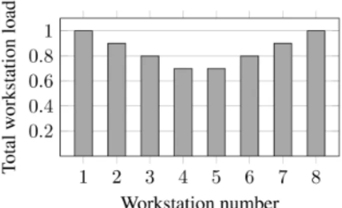
workstation along the line has the shape of a bowl, with times increasing from central station(s). Figure 1 shows an example of such configuration in a line with eight workstations.
Figure 1– Example of a bowl profile. Stations in the center are less loaded than the peripheral ones.
Results presented by Hillier & Boling (1966) considered lines with at most four stations with buffer capacity from one to four units. However, using the exponential distribution does not allow one to tell if the enhancement in the line’s throughput is due to unbalancing the mean or the variability of the task times, since both parameters are the same for that distribution. The investigation of this gap, also considering exponential distribution and assuming some deter-ministic variables, showed the optimum strategy to be a combination of both unbalances (Rao, 1976). The use ofErlangdistribution also produces a bowl load profile as optimum solution and Hillier & Boling (1979) concluded that the effect of the bowl configuration became larger as the number of stations increased. By this time, the first experiments supporting the bowl phenomenon as proposed by Hillier & Boling (1966) were performed.
At one moment, conflicting results related to the production rate and the idle time of the worksta-tions were presented. Some of them argued that an increasing workload profile would be better than a bowl shaped workload. In this sense, (Kottas & Lau, 1981) proposed an approach for studying and monitoring the transient behavior of an assembly line and showed that the conflict-ing results were, in fact, underestimated transient properties read as steady-state behavior.
Another controversy happened when Smunt & Perkins (1985), using some results from (Dudley, 1963), argued that the assembly lines considered in previous researches, with few stations and high variability, were not of practical interest. They then presented results for more realistic sce-narios that supported a degradation of the line’s throughput if a bowl workload profile was used. Nevertheless, (Karwan & Philipoom, 1989) and (So, 1989), independently argued that (Smunt & Perkins, 1985) had some flaws in their experimental design. All the group of researchers agreed that more realistic scenarios should be explored.
Hillier & Hillier (2006) optimized workload and buffers capacity simultaneously and the results showed that, if the buffers are small, their optimum allocation is balanced and the workload should follow a bowl pattern. Considering one wants to minimize total time, idle time or mean time of a product in the system, (Das, Garcia-Diaz, MacDonald & Ghoshal, 2010) and (Das, Sanchez-Rivas, Garcia-Diaz & MacDonald, 2010), using simulation, explored bowl, inverted bowl and crescent workload profiles. Also, in (Das et al., 2012) there is a comparison between crescent and decrescent load profile. Furthermore, optimizing buffer capacity between stations and work allocation using exact and heuristic methods was studied by Hillier (2013).
It is important to state that none of the articles cited above considered the indivisibility of the tasks, even though this is a strong requirement in most practical situations. In other words, all authors have assumed that a task with a specific size is always available to fulfill the required workload of a station. This flaw has been already pointed out by Tempelmeier (2003) but, to the best of our knowledge, no investigation was conducted to settle this question. This is one of the main research gaps explored in the remainder of this article.
In general, the innovation presented in this paper is twofold. First, we use a simulation model to try to conclude on the existence of the bowl effect in larger lines and with more diversified configurations. For this, we use the set of instances recently proposed by Otto et al. (2013) while considering the integrality of the tasks. We also propose a simple MIP methodology to generate bowl format configurations for lines with homogeneous and heterogeneous workforce, either by introducing load unbalances or by analysing the effect of unbalances in deviation. These two cases are described in the following.
2.1.1 Load unbalance
Constraints (3) and (11) are appropriate for the deterministic scenario because they induce a uniform load distribution among all workstations, hence minimizing the cycle timeC. In order to obtain bowl-like solutions, these constraints are modified in the corresponding models. For SALBP the new constraints are:
i∈N
ti·xis ≤αsC, ∀s∈S, (15)
and for ALWABP, the cycle time constraints are replaced by:
i∈N
w∈W
pwi·xswi ≤αsC, ∀s∈S, (16)
in both cases, as are parameters whose values respect the following equations:
α1>0, (17)
αs =α|S|−s+1, s=1. . .⌊|S|/2⌋. (18)
Constraints (17) guarantee positive loads for workstations while constraints (18) induce sym-metry in the load configuration. Finally, constraints (19) define the bowl slope level which is controlled by parameterβ, 0< β≤1. Note that ifβ =1 the proposed models are equivalent to the original ones.
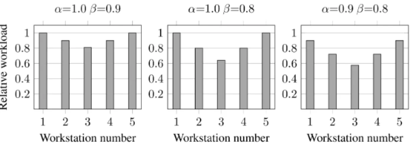
Figure 2 shows examples of resulting profiles for some values ofαandβ.
Figure 2– Load configurations for different values of parametersαandβ.
2.1.2 Deviation unbalance
Other characteristic that may induce a bowl effect is related to task times deviations. Letcs = µσss
indicate the level of variability in a given station execution’s time s ∈ S. A bowl profile is obtained by maintaining the station loads fixed and reducing the task deviation times in central stations. The deviation was computed considering solutions without restrictions (15) or (16) and by artificially adjusting task deviation times from the base case.
The base case considers σµ = 0.1, s = 1, . . . ,S, while bowl profiles are obtained withcs =
θcs−1,s = 1, . . . ,⌊|S|/2⌋andcs =c|S|−s+1,s =2, . . . ,⌊|S|/2⌋ −1, where 0 < θ ≤ 1 is a
parameter related to the depth of the bowl. Note that these equations are similar to the equations to generate bowl solutions for the mean case. Hence, the bowl profiles for mean and deviation have the same shapes.
3 SIMULATION MODEL
Simulation is a technique for performance and reaction analysis of a system. It can be useful in planning stages or when the system is already in operation if careful validation on practical contexts is desired (Leal et al., 2011). Most benefits of simulation appear in contexts in which the system under study has many features that can not be modelled properly with the use of other analytical techniques due, for example, to its complexity.
distributions, each one representing a process in the model. Then, a statistical sampling is used to summarize the result for each input. In other words, simulation models can be used to analyze processes having a degree of uncertainty (randomness) in their variables (Kroese, 2008).
In this work, the simulation model built in order to evaluate assembly lines has the number of products which left the line as a state-variable, it is of continuous time, discrete state, stochastic, linear, dynamic, open and unstable (Ross 2006). Also, it is a next-event analysis model whose events are triggered when a station finishes its work.
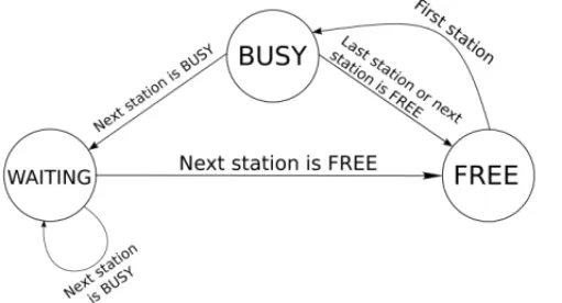
Actually, besides the starting event, there is just one more type of event that happens during a simulation: when all the work in a station has been done, a previously scheduled event is triggered and the product is delivered to the next station or the current station gets blocked, following the diagram in Figure 3. There are three possible workstation states. Any transition can only happen when the referred event is triggered. Namely, whenever the event happens, if the current station is in BUSY state it checks the following station, if it is in FREE state, the finished piece of product is delivered to it and the state of the current station changes to FREE, which means it can receive another piece to work on, if it is the first station it returns to BUSY state (there is always work available for the first station); otherwise, if the next station is in BUSY state when the current finishes its work, the current station changes its state to WAITING, blocking itself until the next station is FREE. If the current BUSY station is the last station of the line it changes its state to FREE, since there is no need to check for the next station’s state. There is also one action, not shown in Figure 3, that takes place when the transition from BUSY to FREE happens: the current station changes the state of the next station to BUSY, translating the fact that a new piece of product arrived in the following station. Hence, the event triggered when a workstation finishes its work controls the flow of products in the line.
Figure 3 – Simplified machine state for the workstations. When a workstation is in BUSY state it is performing some work, in WAITING state it is blocked and in FREE it is starved.
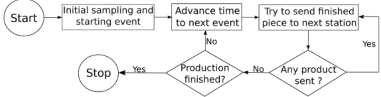
time. The handling of scheduled events is performed according to the diagram shown in Figure 4 which has been adapted from (Robinson 2004).
Figure 4– Flowchart of a simulation. The simulation advances its time to the next scheduled event and process the corresponding events. If none of them can be processed it advances time again until at least one station is not blocked. Simulation stops when a specified number of completed products is reached.
When a simulation starts, every station state is set to FREE, but the first one whose state is set to BUSY, hence an event corresponding to finishing the first job in the first station is scheduled. Then, time is advanced to the next event which is processed according to diagram in Figure 3. If no station can pass the product to the next station and the desired number of products is not yet reached, the simulation advances to the next scheduled event until a workstation becomes able to deliver its work to the following one. The simulation stops when the specified production is reached.
The allocation of tasks to workstations and, in ALWABP case, workers to workstations is given by the respective deterministic mathematical model whose objective is to minimize the assembly line’s cycle time. Since, in the simulation model of this work, every task is supposed to be performed in a time following a normal distribution, two parameters are needed in order to fully specify the task times to the simulation model: meanµ and standard deviationσ. The mean is assumed to be the deterministic time of the task and the standard deviation isσ = 10µ for load unbalance simulations and is given according to subsection 2.1.2 for deviation unbalance simulations.
In summary, we propose a stochastic simulation model using next-event analysis and determinis-tic mathemadeterminis-tical programming models to study the bowl phenomenon considering integer tasks and instances proposed by (Otto et al., 2013) and (Chaves et al., 2009), respectively for SALBP and ALWABP. The results obtained in the experiments are detailed in the next section.
4 COMPUTATIONAL RESULTS
2004). All the task times were assumed to follow a Normal distribution,N(µ, σ2), and separated experiments were performed to evaluate the mean and standard deviation unbalances on total workstation load. In order to analyze mean unbalances, experiments withα1 = 1 and β ∈
B = {1.00, 0.99, 0.98, 0.97, 0.96, 0.95, 0.94}were performed (as defined in constraints (17) and (19)); for deviation unbalances the experiments consideredθ∈ {θi =βi|∀βi ∈ B}.
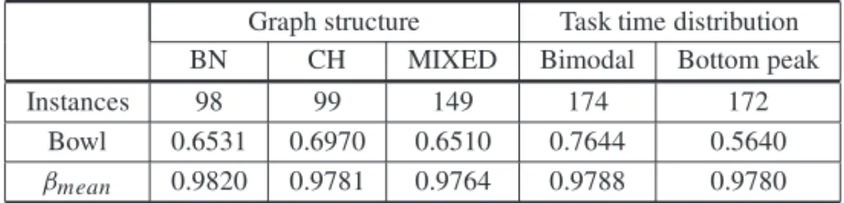
Both SALBP and ALWABP cases were considered independently. The benchmark problems for the SALBP simulations are a subset of the dataset proposed by (Otto et al., 2013). We use the instances for which the known upper bound on the number of stations is seven or less. The benchmark for the ALWABP simulations are the instances of type Heskia and Roszieg from (Chaves et al., 2009). Both, SALBP and ALWABP instances, were solved to optimality. The results’ analysis, performed in the following, focus on the SALBP problems since their instances are more representative than their ALWABP counterparts. Tables 1 through 6 summarize results for the SALBP simulations. Each table presents the total number of instances in the correspond-ing categories, the number of instances in which the bowl phenomenon could be observed (i.e., the number of instances in which the bowl configuration was statistically superior to their bal-anced counterparts) and their meanβ (orθ) for mean (or standard deviation) unbalances. The categories are related to different precedence graph structures and how the task times are dis-tributed: graphs may havebottlenecktasks and chaintasks and, according to the relevance of one or other type of tasks, Otto et al. (2013) classified the graph structure asBN(forbottleneck), CH(forchain) orMIXED when there is no prominent characteristic. Task time’s distributions may be bimodal or with peak at small tasks (bottom peak) in the considered instances. Also a statisticalt-test with 0.05 threshold in the p-value was used to ensure statistical difference from the best bowl solution to the balanced one.
Tables 1, 2 and 3 contain results related to the mean unbalance simulations. Table 1 presents the results grouped by number of stations. Most of the instances (163) considered have three work-stations in the optimal solution and in 53.99% the best bowl solution was statistically different from the balanced solution leading toβmean =0.9781. The deepest mean bowl was also found in
instances with four workstations which was, as well, the case that present greater relative number of observable bowl phenomenons (84.21%).
Table 1– Mean unbalance results for SALBP instances grouped by number of workstations.
Workstations
3 4 5 6 7
Instances 163 38 89 50 6
Bowl 0.5399 0.8421 0.7416 0.7800 0.8333 βmean 0.9781 0.9781 0.9788 0.9777 0.9900
Table 2– Mean unbalance results for SALBP instances grouped by graph structure and task time distribution.
Graph structure Task time distribution BN CH MIXED Bimodal Bottom peak
Instances 98 99 149 174 172
Bowl 0.6531 0.6970 0.6510 0.7644 0.5640 βmean 0.9820 0.9781 0.9764 0.9788 0.9780
The bottom peak task time distribution presented the deepest bowl and bimodal instances shown a greater number of solutions for which the bowl configuration was more productive. Also, it can be seen thatCHgraphs and bimodal task distribution seem to favor the occurrence of the bowl phenomenon.
Table 3 presents the results considering both number of stations and graph structure and number of stations and task time distribution. In some of these scenarios there was no available instance: three workstations with bimodal task time distribution and five workstations with bottom peak time distribution, for example. Therefore, there are table cells marked with “–” where the corre-sponding result is not applicable. Again, for three and four workstation, it is possible to seeCH graphs favouring the bowl phenomenon, nevertheless, this is not true for five workstations. It is hard to draw conclusions for instances with seven workstations since there are fewer instances in this scenario. Likewise, for task time distribution case the instances are not well suited for comparing bimodal and bottom peak distributions.
Table 3– Mean unbalance results for SALBP instances combining number of workstation with graph structure or task time distribution.
Workstations Graph structure Task time distribution BN CH MIXED Bimodal Bottom peak
Instances 47 46 70 0 163
3 Bowl 0.5319 0.5435 0.5429 – 0.5399
βmean 0.9832 0.9772 0.9753 – 0.9781
Instances 11 12 15 29 9
4 Bowl 0.6364 1.0000 0.8667 0.7931 1.0000
βmean 0.9800 0.9792 0.9762 0.9783 0.9778
Instances 28 24 37 89 0
5 Bowl 0.7857 0.7083 0.7297 0.7416 –
βmean 0.9818 0.9770 0.9774 0.9788 –
Instances 10 15 25 50 0
6 Bowl 0.8000 0.8667 0.7200 0.7800 –
βmean 0.9788 0.9785 0.9767 0.9777 –
Instances 2 2 2 6 0
7 Bowl 1.0000 1.0000 0.5000 0.8333 –
Tables 4, 5 and 6 present results regarding bowl profiles in cs = µσss. Table 4 shows results
grouped by number of workstations. Instances with five, six and seven workstations achieved 100% ofbowl phenomenon occurrence(i.e., in all cases the lines with the obtained bowl con-figurations were more productive than their balanced counterparts). Also, the mean depth of the bowl for seven workstation reached the maximum value among all the experiments conducted.
Table 4 – Deviation unbalance results for SALBP instances grouped by number of workstations.
Workstations
3 4 5 6 7
Instances 163 38 89 50 6
Bowl 0.5337 0.9737 1.0000 1.0000 1.0000 θmean 0.9480 0.9462 0.9402 0.9410 0.9400
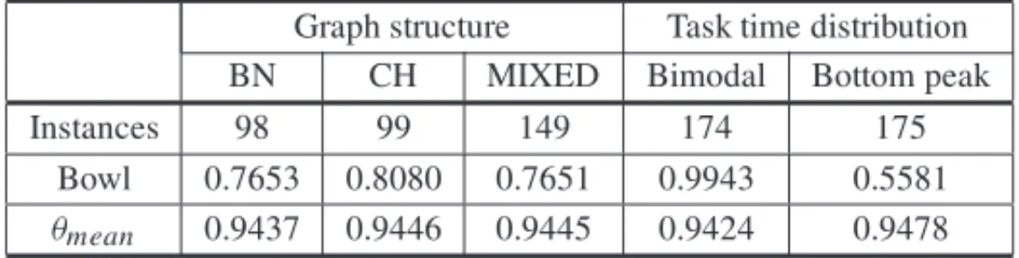
Table 5 presents results grouped by graph structures and task time distributions. In the graph structure group, the deepest mean bowl was found in thebottleneck class and the class that presented the greater relative number of bowl-shaped solution performing better than balanced solutions was thechainone. The bimodal task time distribution presented deepest and greater number of better bowl solutions. Four out of five classes presented more than 75% of occurrence of the bowl phenomenon, reaching 99.43% in the bimodal class.
Table 5– Deviation unbalance results for SALBP instances grouped by graph structure and task time distribution.
Graph structure Task time distribution BN CH MIXED Bimodal Bottom peak
Instances 98 99 149 174 175
Bowl 0.7653 0.8080 0.7651 0.9943 0.5581 θmean 0.9437 0.9446 0.9445 0.9424 0.9478
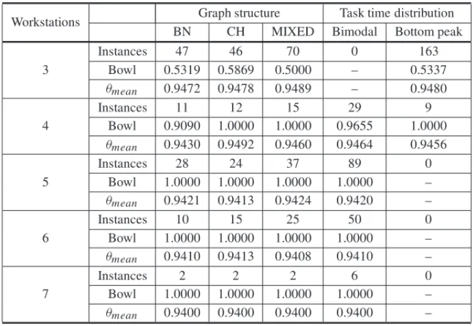
Table 6 summarizes results combining number of workstations and graph structure and number of workstations and task time distribution for deviation analysis. For instances with three work-stations the graph structurechainseems to favor the effect. For instances with more than three stations the phenomenon could be observed in most of the problems and the maximum bowl depth considered in the experiments was reached in a number of scenarios.
Regarding the ALWABP, the results were analyzed in a much simpler way since the available instances are not as representative as those for the SALBP. Table 7 shows the results. They are grouped by variance among workers: low variance means that task execution time varies less among workers than in the high variance scenario (Chaves et al. 2009). The table presents the fraction of instances where the bowl phenomenon could be observed and βmean for mean
unbalance or θmean for deviation unbalance. For each class (low and high) 80 instances were
Table 6– Deviation unbalance results for SALBP instances combining number of work-station with graph structure or task time distribution.
Workstations Graph structure Task time distribution BN CH MIXED Bimodal Bottom peak
Instances 47 46 70 0 163
3 Bowl 0.5319 0.5869 0.5000 – 0.5337
θmean 0.9472 0.9478 0.9489 – 0.9480
Instances 11 12 15 29 9
4 Bowl 0.9090 1.0000 1.0000 0.9655 1.0000 θmean 0.9430 0.9492 0.9460 0.9464 0.9456
Instances 28 24 37 89 0
5 Bowl 1.0000 1.0000 1.0000 1.0000 –
θmean 0.9421 0.9413 0.9424 0.9420 –
Instances 10 15 25 50 0
6 Bowl 1.0000 1.0000 1.0000 1.0000 –
θmean 0.9410 0.9413 0.9408 0.9410 –
Instances 2 2 2 6 0
7 Bowl 1.0000 1.0000 1.0000 1.0000 –
θmean 0.9400 0.9400 0.9400 0.9400 –
Table 7– Mean and deviation unbalances for ALWABP instances.
Low High
mean deviation mean deviation Bowl 0.6125 0.8625 0.7500 0.8000 βmeanorθmean 0.9684 0.9423 0.9670 0.9430
Furthermore, in the deviation case the bowl phenomenon was observed in fewer instances if compared to SALBP. Nevertheless, the bowl phenomenon could be observed in more than 50% of the cases for every class (and case) considered.
As a final note, we remark that the SALBP and ALWABP results show that the bowl phenomenon regarding variability occurred in more instances than the effect regarding mean. This may have happened because there is no integrality constraint in the standard deviation whereas, for the mean case, the proposed MIP formulation considers the integrality of the tasks.
5 CONCLUSIONS
pre-vious bowl phenomenon studies, favoring the generalization of the conclusions obtained. These conclusions indicate that assembly lines can indeed benefit from bowl shaped configurations even if the more realistic scenario with indivisible tasks is considered.
ACKNOWLEDGMENTS
This work was developed with financial support fromCNPq,CAPES/DGU(258-12) andFAPESP.
REFERENCES
[1] ARAUJO´ FFB, COSTA AM & MIRALLESC. 2012. Two extensions for the assembly line worker assignment and balancing problem: parallel stations and collaborative approach.International Jour-nal of Production Economics,140: 483–495.
[2] ARAUJO´ FFB, COSTAAM & MIRALLESC. 2014. Balancing parallel assembly lines with disabled workers.European Journal of Industrial Engineering, (in press).
[3] BARTENK. 1962. A queuing simulator for determining optimum invetory levels in a sequential pro-cess.Journal of Industrial Engineering,14: 703–710.
[4] BATTA¨IA O & DOLGUI A. 2012. A taxonomy of line balancing problems and their solution approaches.International Journal of Production Economics.
[5] BAYBARSI. 1986. A Survey of Exact Algorithms for the Simple Assembly Line Balancing Problem.
Management Science,32: 909–932.
[6] BLUMC & MIRALLESC. 2011. On solving the assembly line worker assignment and balancing problem via beam search.Computers & Operations Research,38: 328–339.
[7] BORBAL & RITTM. 2014. A heuristic and a branch-and-bound algorithm for the Assembly Line Worker Assignment and Balancing Problem.Computers & Operations Research,45: 87–96.
[8] BOYSENN & FLIEDNER M. 2008. A versatile algorithm for assembly line balancing.European Journal of Operational Research,184: 39–56.
[9] BOYSENN, FLIEDNERM & SCHOLLA. 2007. A classification of assembly line balancing problems.
European Journal of Operational Research,183: 674–693.
[10] BOYSENN, FLIEDNER M & SCHOLLA. 2008. Assembly line balancing: Which model to use when?.International Journal of Production Economics,111: 509–528.
[11] CHAVESAA, LORENALAN & MIRALLES C. 2009. Hybrid metaheuristic for the assembly line worker assignment and balancing problem.Lecture Notes on Computer Science,5818: 1–14.
[12] COSTA AM & MIRALLES C. 2009. Job rotation in assembly lines employing disabled workers.
International Journal of Production Economics,120: 625–632.
[13] DAS B, GARCIA-DIAZA, MACDONALDCA & GHOSHALKK. 2010. A computer simulation approach to evaluating bowlversusinverted bowl assembly line arrangement with variable opera-tion times.The International Journal of Advanced Manufacturing Technology, pp. 15–24.
[15] DASB, SANCHEZ-RIVASJM, GARCIA-DIAZA & MACDONALDCA. 2010. A computer sim-ulation approach to evaluating assembly line balancing with variable operation times. Journal of Manufacturing Technology Management,21: 872–887.
[16] DUDLEYN. 1963. Work-time distributions.International Journal of Production Research,2: 137– 144.
[17] GHOSHS & GAGNONRJ. 1989. A comprehensive literature review and analysis of the design, balancing and scheduling of assembly systems.International Journal of Production Research,27: 637–670.
[18] HILLIERFS & BOLINGRW. 1966. The effects of some design factors on the efficiency of production lines with variable operation times.Journal of Industrial Engineering,17: 651–658.
[19] HILLIERFS & BOLINGRW. 1979. On the Optimal Allocation ofWork in Symmetrically Unbalanced Production Line Systems with Variable Operation Times.Management Science,25: 721–728.
[20] HILLIER FS & SO KC. 1996. On the robustness of the bowl phenomenon.European Journal of Operational Research,2217: 496–515.
[21] HILLIERM. 2013. Designing unpaced production lines to optimize throughput and work-in-process inventory.IIE Transactions,45: 516–527.
[22] HILLIERMS & HILLIERFS. 2006. Simultaneous optimization of work and buffer space in unpaced production lines with random processing times.IIE Transactions,38: 39–51.
[23] KARWANK & PHILIPOOMP. 1989. A note on “Stochastic unpaced line design: Review and further experimental results”.Journal of Operations Management,8: 48–54.
[24] KOTTASJF & LAUH-S. 1981. Some problems with transient phenomena when simulating unpaced lines.Journal of Operations Management,1: 155–164.
[25] KROESERYRDP. 2008.Simulation and The Monte Carlo Method, 2nd ed., John Wiley & Sons, Inc.
[26] LEALF, COSTARFDS, MONTEVECHIJAB,DEALMEIDADA & MARINSFAS. 2011. A practical guide for operational validation of discrete simulation models.Pesquisa Operacional,31: 57–77.
[27] MAHAJANPS & INGALLSRG. 2004. Evaluation of methods used to detect warm-up period in steady state simulation.Proceedings of the 2004 Winter Simulation Conference, pp. 663–671.
[28] MIRALLES C, GARCIA-SABATERJP, ANDRES´ C & CARDOSM. 2007. Advantages of assembly lines in Sheltered Work Centres for Disabled. A case study.International Journal of Production Economics,110: 187–197.
[29] MOREIRAMCO & COSTA AM. 2013. Hybrid Heuristics for planning job rotation in Assembly Lines with disabled workers.International Journal of Production Economics,141: 552–560.
[30] MOREIRAMCO, RITTM, COSTAAM & CHAVESAA. 2012. Simple heuristics for the assembly line worker assignment and balancing problem.Journal of heuristics,18: 505–524.
[31] MUTLUO, POLATO & SUPCILLERAA. 2013. An iterative genetic algorithm for the assembly line worker assignment and balancing problem of type-II.Computers & Operations Research,40: 418–426.
[33] PATTERSONR. 1964. Markov processes occurring in the theory of traffic flow through an N-Stage stochastic service system.Journal of Industrial Engineering,15: 188–193.
[34] RAONP. 1976. A generalization of the ’bowl phenomenon’ in series production systems. Interna-tional Journal of Production Research,14: 437–443.
[35] ROBINSONS. 2004.Simulation – the practice of model development and use. John Wiley & Sons.
[36] ROSSSM. 2006.Simulation. Elsevier.
[37] SALVESONME. 1955. The assembly line balancing problem.Journal of Industrial Engineering,6: 18–25.
[38] SCHOLLA. 1999.Balancing and sequencing of assembly lines. Physica-Verlag.
[39] SCHOLLA & BECKERC. 2006. State-of-the-art exact and heuristic solution procedures for simple assembly line balancing.European Journal of Operational Research,168: 666–693.
[40] SCHOLLA, FLIEDNERM & BOYSENN. 2010. Absalom: Balancing assembly lines with assignment restrictions.European Journal of Operational Research,200: 688–701.
[41] SMUNTTL & PERKINSWC. 1985. Stochastic unpaced line design: Review and further experimental results.Journal of Operations Management,5: 351–373.
[42] SOKC. 1989. On the efficiency of unbalancing production lines.International Journal of Production Research,27: 717–729.
[43] TEMPELMEIERH. 2003. Practical considerations in the optimization of flow production systems.
International Journal of Production Research,41: 149–170.
[44] TONGEFM. 1961.A heuristic program for assembly line balancing. Prentice-Hall, Englewood Cliffs, NJ.