Uma classe mais flexível de modelos semiparamétricos para dados de sobrevivência

Fábio Nogueira Demarqui

Uma classe mais flexível de modelos

semiparamétricos para dados de sobrevivência

Belo Horizonte - MG

Fábio Nogueira Demarqui

Uma classe mais flexível de modelos

semiparamétricos para dados de sobrevivência

Tese de doutorado apresentada ao Departa-mento de Estatística do Instituto de Ciên-cias Exatas da Universidade Federal de Mi-nas Gerais, como requisito parcial à obtenção do título de Doutor em Estatística.

Orientadora:

Rosangela H. Loschi

Co-orientadores:

Enrico A. Colosimo & Dipak K. Dey

Doutorado em Estatística Departamento Estatística Centro de Ciências Exatas Universidade Federal Minas Gerais

Belo Horizonte - MG

i

Ao meu irmão,

ii

Agradecimentos

A minha família, pelo exemplo e apoio incondicional. Vocês são a razão da minha força e inspiração para seguir sempre em frente.

À Graici, por simplesmente fazer parte da minha vida.

A Rosangela e o Enrico, pela orientação, confiança e, sobre tudo, pela amizade que se formou no decorrer desses quase 6 anos de trabalho em conjunto. Fico com a certeza de que ainda temos muito trabalho pela frente.

Ao professor Dipak Dey, pela excelente acolhida, e, principalmente, pela grande opor-tunidade que me proporcionou ao aceitar-me em seu departamento. Tenho aprendido muito com o Sr., Dr. Dey. Gostaria de agradecer também aos funcionários e colegas do departamento de Estatística da UCONN por toda hospitalidade e ajuda.

Aos professores do Departamento de Estatística da UFMG, em especial a Denise, Frederico, Gregório, Luiz, Marcelo, Mercedes e Renato. Gostaria também de agradecer a todos os funcionários do Departamento de Estatística, em particular a Cristina, Marcinha, Rogéria e Rose.

À Maristela, amiga de todas as horas, meu agradecimento especial, pelo companhei-rismo, por ter me ajudado em tudo um pouco, e pelas nossas infindáveis discussões. Se estas, na maioria das vezes não nos levou a lugar algum, pelo menos nos divertimos a valer.

Ao Marcos, Rafael (Waldo) e Nathalie, por toda a ajuda durante o período em que visitei os EUA, e, principalmente, pela amizade que se formou entre nós. Guardo vocês no coração.

Ao Max, Rodrigo e Juan, pelas inumeras discussões sobre o trabalho da tese, ou simplesmente por me ouvirem nos meus momentos de devaneios.

iii

iv

"A razão cardeal de toda a superioridade humana é sem dúvida a vontade. O poder

nasce do querer. Sempre que o homem aplicar a veemência e a perseverante energia de

sua alma a um fim, ele vencerá os obstáculos e, se não atingir o alvo, pelo menos fará

coisas admiráveis."

v

Resumo

vi

Abstract

vii

Introdução

O avanço computacional observado principalmente nas duas últimas décadas, aliado à disponibilidade de algoritmos computacionais mais eficientes, tem possibilitado sobre-maneira o desenvolvimento de métodos estatísticos para a análise de dados com estru-turas cada vez mais complexas. Em análise de sobrevivência, este recente desenvolvi-mento tecnológico tem impulsionado o desenvolvidesenvolvi-mento de modelos semiparamétricos e não-paramétricos como alternativas mais flexíveis e robustas aos modelos paramétricos. Em particular, abordagens Bayesianas para a modelagem de dados de sobrevivência tem recebido lugar de destaque na literatura recente. Seguindo essas tendências, e adotando o enfoque Bayesiano, nesta tese de doutorado são propostas algumas extensões, com enfoque Bayesiano, do Modelo Exponencial por Partes (MEP), incluindo a modelagem direta da função risco, modelos de regressão semi-parametricos e modelos com fração de cura.

viii

O MEP é caracterizado pela aproximação da função risco por segmentos de retas cujos comprimentos são determinados por uma grade de pontos que divide o eixo do tempo em um número finito, digamos b, de intervalos. Para construirmos este modelo, precisamos especificar uma grade de pontos, digamos τ ={s0, s1, ..., sb}, tal que 0 =s0 < s1 <· · ·< sb < ∞. Esta grade τ induz uma partição do eixo do tempo em intervalos contíguos da forma Ij = (sj−1, sj], dentro dos quais assumimos uma taxa de falha constante, λj, j = 1,· · · , b. Logo, a função risco, avaliada num tempo t >0, é aproximada por:

h(t) =λj, t∈Ij = (sj−1, sj], j = 1,· · · , b.

Existem vários trabalhos que discutem propriedades e extensões do MEP. Friedman (1982) faz uso do MEP para modelar a função de risco de base do modelo de Cox, e apresenta condições para a existência e distribuição assintótica dos estimadores de má-xima verossimilhanca (EMV) para as taxas de falha e coeficientes da regressão. Kim e Proschan (1991) discutem algumas vantagens do MEP sobre o estimador de Kaplan-Meyer para a função de sobrevivência para dados sem covariáveis. Barbosa et al. (1996) aplicam métodos usados em modelos lineares generalizados para ajustar dados de tempos de vida acelerados utilizando o MEP. O método da máxima verossimilhanca também é empregado por Chen e Ibrahim (2001) para ajustar modelos com fração de cura utilizando o MEP na presença de dados faltantes. A literatura Bayesiana relacionada ao MEP tam-bém é bastante extensiva. Gamerman (1991) estende o modelo de Cox propondo uma abordagem dinâmica para modelar dados de sobrevivência em que os efeitos de variáveis explicativas variam ao longo do tempo. Sahuet al.(1997) usa o MEP para modelar dados de sobrevivência multivariados. Em tal trabalho, fragilidades (i.e., efeitos aleatórios) são consideradas para acomodar a correlação inerente aos tempos de sobrevivência de ele-mentos pertencentes a um mesmo grupo, e um processo correlacionado é assumido para modelar a incerteza sobre as taxas de falha do MEP. Uma breve revisão sobre algumas abordagens com enfoque Bayesiano para o MEP pode ser encontrada em Ibrahim et al. (2001b).

ix

modelo, a grade τ = {s0, s1, ..., sb} tem sido escolhida de maneira arbitrária na maioria dos trabalhos disponíveis, entre os quais os citados anteriormente. Kalbfleisch e Prentice (1973) sugerem que a escolha da grade deveria ser feita independentemente dos dados, mas não apresentam um procedimento para tanto. Breslow (1974) propõe que se tome os pontos finais sj dos intervalos Ij = (sj−1, sj] como sendo iguais aos tempos de falha observados. Outras discussões heurísticas com respeito a possíveis escolhas para a grade τ ={s0, s1, ..., sb}podem ser encontradas em Gamerman (1991), Sahuet al.(1997) e Qiou et al.(1999), entre outros.

Na prática, o problema de especificarmos uma grade apropriada para o ajuste do MEP pode ser resolvido assumindo-se que τ = {s0, s1, ..., sb} é uma quantidade aleatória. O primeiro esforço efetivo nesta direção é devido a Arjas e Gasbarra (1994). Estes autores assumen que os pontos finais dos intervalosIj = (sj−1, sj]são definidos de acordo com um processo de saltos que seguem uma estrutura de martingal, a qual é incluída no modelo através das distribuiçõesa priori. Extensões desta abordagem podem ser encontradas em McKeague e Tighiouart (2000) and Kimet al. (2006).

Apesar do uso de um processo de Poisson homogêneo (PPH) fornecer uma solução para a questão da modelagem do MEP com grade aleatória, esta estratégia apresenta alguns inconvenientes. Primeiro, tal abordagem não possibilita a modelagem direta da grade que define o MEP, não sendo possível, desta forma, que a mesma seja estimada. Além disso, na ausência de qualquer informaçãoa priorisobreλj, para queλj seja estimável é necessário que cada intervalo Ij = (sj−1, sj] contenha pelo menos um tempo de falha. Embora esta condição possa ser relaxada assumindo-se um processo correlacionado para a função risco (veja, por exemplo, Gamerman (1991, 1994) e Ibrahimet al.(2001b)), intervalos contendo pelo menos um tempo de falha são preferíveis no processo de estimação. Ademais, a disposição dos tempos de falha sob o eixo do tempo não é diretamente considerada nesta abordagem. Finalmente, assumindo de um PPH para gerarmos o número de intervalos e seus respectivos pontos finais, o número total de parâmetros do modelo passa a ser aleatório, tornando necessário o uso de um algoritmo MCMC com saltos reversíveis.

x

tal abordagem, a modelagem da grade é feita levando-se em conta a disposição dos tem-pos de falha sob o eixo do tempo, e a existência de pelo menos um tempo de falha em cada intervalo induzido pela grade aleatória do MEP é garantida. Além disto, apesar de o número de parâmetros a serem estimados poder variar, esta forma de modelagem mantem fixado o número máximo de parâmetros do modelo. Além disso, a abordagem proposta por Demarqui et al. (2008) pode ser estendida em diversas direções, como por exemplo no ajuste de modelos com covariáveis dependentes do tempo e/ou efeitos das covariáveis mudando ao longo do tempo, modelos com fração de cura, modelos de fragilidade para dados de sobrevivência multivariados e/ou espacialmente correlacionados, entre outros, abrindo, desta forma, um novo leque de pesquisa envolvendo o MEP.

Esta tese é composta por quatro artigos. Em todos esses trabalhos, extensões da abordagem proposta por Demarqui et al. (2008) para a modelagem da grade do MEP são consideradas. A metodologia proposta neste trabalho é bastante geral, podendo ser aplicada para dados do tipo tempo até a ocorrência de um evento de interesse oriundos de qualquer área do conhecimento. Entretando, é dado enfoque nesta tese à aplicações ori-undas da área médica, especificamente, de dados de sobrevivência referentes a indívíduos diagnosticados com câncer. A suposição básica para a aplicabilidade dos modelos aqui propostos é que os tempos de sobrevivência sejam censurados à direita, ou seja, os tempos até a ocorrência do evento de interesse são maiores ou iguais aos tempos observados, e que o mecanismo gerador das censuras seja não informativo. A abordagem proposta também é apropriada para dados de sobrevivência com a presença de empates. A contribuição de cada artigo é resumida a seguir.

xi

quiet al. (2008), o modelo apresentado no primeiro artigo, e as abordagens introduzidas por Gamerman (1994) e Ibrahimet al. (2001a). A análise dos tempos de sobrevivência de indivíduos diagnosticados com câncer no cérebro no condado americano de Windham-CT, EUA, é novamente apresentada como ilustração dos modelos propostos. As comparações entre os modelos ajustados considerando-se grades fixas e aleatórias, bem como diferentes distribuições a priori para a taxa de falha, são realizadas utilizando-se como medida de comparação a média do logaritmo da pseudo-verossimilhança marginal (veja Ibrahim et al.(2001b) e referências).

O terceiro artigo trata-se de modelos de regressão semiparamétricos com variáveis explicativas com efeito agindo multiplicativamente na função risco. O modelo proposto neste artigo pode ser visto como uma extensão do modelo de riscos proporcionais pro-posto por Cox (1971), em que é permitido que covariáveis e ou seus correspondentes efeitos variem ao longo do tempo, e incluí como caso especial o modelo dinâmico in-troduzido por Gamerman (1991). A análise dos tempos de sobrevivência de indivíduos diagnosticados com câncer no cérebro no condado americano de Windham-CT é nova-mente apresentada como ilustração, considerando-se o sexo dos pacientes como variável explicativa. Para avaliar-se o desempenho do modelo segundo diferentes especificações a priori, considerando-se grades fixas e aleatórias para o MEP, são utilizados o fator de Bayes e as probabilidades a posteriori de cada modelo (veja Kass e Raftery (1995) e Ibrahimet al. (2001b), entre outros).

diagnostica-xii

Modeling survival data using the piecewise exponential

model with random time grid

Fabio N. Demarqui

_{, Dipak K. Dey}

_,

Rosangela H. Loschi

_{and Enrico A. Colosimo}

1

_{Universidade Federal de Minas Gerais, Brazil,}

email:{fndemarqui, loschi, enricoc}@est.ufmg.br

2

_{University of Connecticut, USA,}

emai: dey@stat.uconn.edu

Abstract

In this paper we present a fully Bayesian approach to model survival data using the piecewise exponential model with random time grid. We assume a joint noninformative improper prior distribution for the time grid and the failure rates of the PEM, and show how the clustering structure of the product partition model can be adapted to accommodate improper prior distributions in the framework of the PEM. Properties of the model are discussed and the use of the proposed methodology is exemplified through the analysis of a real data set. For comparison purposes, the results obtained are compared with those provided by other methods existing in the literature.

Keywords: Bayesian inference, Gibbs sampler, piecewise exponential model, product partition model, survival analysis.

1

Introduction

the PEM can be thought as a nonparametric model as far as it does not have a closed form for the hazard function. This nice characteristic of the PEM allows us to use this model to approximate satisfactorily hazard functions of several shapes. For this reason, the PEM has been widely used to model time to event data in different contexts, such as clinical situations including kidney infection Sahu et al. (1997), heart transplant data Aitkin et al. (1983), hospital mortality data Clark and Ryan (2002), and cancer studies including leukemia Breslow (1974), gastric cancer Gamerman (1991), breast cancer Ibrahim et al. (2001) (see also Sinha et al. (1999) for an application to interval-censored data), melanoma Kim et al. (2006) and nasopharynx cancer McKeague and Tighiouart (2000), among others. The PEM has also been used in reliability engineering (Kim and Proschan, Kim and Proschan (1991), Gamerman, Gamerman (1994)), and economics problems Gamerman (1991), Bastos and Gamerman (2006).

In order to construct the PEM, we need to specify a time grid which divides the time axis into a finite number of intervals. Then, for each interval induced by that time grid, we assume a constant failure rate. Thus, we have a discrete version, in the form of a step function, of the true and unknown hazard function.

The time gridτ ={s0, s1, ..., sJ}plays a central role in the goodness of fit of the PEM. It is well know that a time grid having a too large number of intervals might provide unstable estimates for the failure rates, whereas a time grid based on just few intervals might produce a poor approximation for the true survival function. In practice, we desire a time grid which provides a balance between good approximations for both the hazard and survival functions. This issue has been one of the greatest challenges of working with the PEM. Although there exist a vast literature related to the PEM, the time grid τ = {s0, s1, ..., sJ} has been arbitrarily chosen in most of those works. Kalbfleisch and Prentice (1973) suggest that the selection of the time gridτ ={s0, s1, ..., sJ}should be made independent of the data, but they do not provide any procedure to do such. Breslow (1974) proposes defining the endpoints sj of the intervals Ij = (sj−1, sj] as the observed failure times. We shall refer the PEM constructed based on such time grid to as nonparametric PEM. Other heuristic discussions regarding adequate choices for the time grid of the PEM can be found in Gamerman (1991), Sahu et al. (1997) and Qiou et al. (1999), to cite few.

assuming independent gamma prior distributions for the failure rates, they prove that the prior distribution for the time grid has a product form, and use the structure of the Product Partition Model (PPM) proposed by Barry and Hartigan (1992) to handle the problem. By considering such approach, the use of the reversible jump algorithm to sample from the posteriors is avoided althought the dimension of the parametric space is not fixed.

In this paper we extend the approach proposed by Demarqui et al. (2008) by deriving a noninformative joint prior distribution for ( λ_{, τ). Specifically, we assume a discrete} uni-form prior distribution for the random time grids of the PEM and then, conditionally on those random time grids, we build the joint Jeffreys’s prior for the failure rates. Conditions regarding the properties of the joint posterior distribution of (λ, τ) are discussed. Finally, we illustrate the usefulness of the proposed methodology by analyzing the survival time of patients diagnosed with brain cancer in Windham-CT, USA, obtained from the SEER (Surveillance, Epidemiology and End Results) database. For comparison purposes, the re-sults are compared with those provided by other methods existing in the literature.

This paper is organized as follows: the proposed model is introduced in Section 2. The new methodology is illustrated with the analysis of a real data set in Section 3. Finally, in Section 4 some conclusion about the proposed model are draw.

2

Model construction

In this section we introduce a piecewise exponential model(PEM) which time grid is a random variable. We start our model presentation reviewing the piecewise exponential distribution.

2.1

Piecewise exponential distribution and the likelihood

Let T be a non-negative random variable. Assume, for instance, that T denotes the time to the event of interest. In order to obtain the probability density function of the PEM we need first to specify a time grid τ ={s0, s1, ..., sJ}, such that 0 = s0 < s1 < s2 < ... < sJ = ∞, which induces a partition of the time axis into J intervals I1 , ..., IJ , where Ij = (sj−1, sj], for j = 1, ..., J. Then, we assume a constant rate for each interval induced byτ, that is:

h(t) =      

    

λ1,if t∈I1; λ2,if t∈I2; ...

λJ,if t∈IJ.

(1)

func-tions as well, we define:

tj =   

 

sj−1, if t < sj−1, t, if t∈Ij, sj, if t > sj,

(2)

where Ij = (sj−1, sj], j = 1, ..., J.

The cumulative hazard function of the PEM is computed from (1) and (2), yielding:

H(t| λ_{, τ) =} J ∑

j=1

λj(tj−sj−1). (3)

Consequently, it follows from the identity S(t) = exp{−H(t)} that the survival function of the PEM is given by:

S(t| λ_{, τ) = exp} {

− J ∑

j=1

λj(tj−sj−1) }

. (4)

The density function of T is obtained by taking minus the derivative of (4). Thus, we say that the random variable T follows a piecewise exponential model with time gridτ and vector parameter λ _{= (λ1, ..., λJ)}′_{, denoted by T ∼ P ED(τ, λ), if its probability density} function is given by:

f(t| λ_{, τ) =λjexp} {

− J ∑

j=1

λj(tj −sj−1) }

, (5)

for t∈Ij = (sj−1, sj] and λj >0, j = 1, ..., J.

Let us assume that n individuals were observed independently. Let Xi be the survival time under study for the i-th element, i = 1., ..., n. Also, assume that there is a right-censoring scheme working independently of the failure process. Denote by Ci the censored time for the the i-th element, and assume that Ci ∼ G, for some continuous distribution G defined on the semi-positive real line. Then, the complete information associated to the process is (Ti, δi), where Ti = min{Xi, Ci} and δi = I(Xi ≤ Ci) are, respectively, the observable survival time, and the failure indicator function for the i-th element. Suppose that (Ti|τ, λ)∼P EM(τ, λ), with τ and λas defined before.

In order to properly construct the likelihood function over the J intervals induced by τ = {s0, s1, ..., sJ}, assume tij as defined in (2). Further, define δij = δiνj(i), where ν

(i) j is the indicator function assuming value 1 if the survival time of the i-th element falls in the j-th interval, and 0 otherwise. It follows that the contribution of the survival time ti ∈Ij = (sj−1, sj] for the likelihood function of the PEM isλ

δij

j exp{− ∑J

given by:

L(D|λ, τ) = n ∏

i=1 ( _J

∏

j=1

λδij_j exp{−λj(tij −sj−1)} )

= J ∏

j=1

λνj_j exp{−λjξj}, (6)

where the number of failures, νj =∑n_l=1δij, and the total time under test observed at each interval Ij, ξj =∑n_i=1(tij −sj−1), are sufficient statistics for λj,j = 1, ..., J.

It is noticeable that, given τ, the likelihood function given in (6) naturally factors into a product of kernels of gamma distributions. As we shall see in the following, along with mild conditions on the joint distribution of the time grid and failure rates, it allow us to use the structure of the PPM proposed by Barry and Hartigan (1992) to model the randomness of the time grid of the PEM.

2.2

Priors and the clustering structure

Following Demarqui et al. (2008), we start our model formulation by imposing some con-strains on the set of possible time grids for the PEM. Specifically, we assume the time grid associated to the nonparametric approach as the finest possible time grid for the PEM. We further assume that only time grids whose endpoints are equal to distinct observed failure times are possible. These assumptions guarantee that at least one failure time falls at each interval induced by the random time grid of the PEM.

The randomness of the time grid of the PEM is modeled through the clustering structure of the PPM as follows. Let F _{= {0, y1, ..., ym} be the set formed by the origin and the} m distinct ordered observed failure times from a sample of size n. Then, F _{defines a} partition of time into disjoint intervals Ij, j = 1, . . . , m, as defined previously. Further, denote by I ={1, ..., m} the set of indexes related to such intervals. Let ρ={i0, i1, ..., ib}, 0 =i0 < i1 < ... < ib =m, be a random partition of I, which divides them initial intervals into B =b new disjoint intervals. The random variable B denotes the number of clustered intervals related to the random partition ρ. Finally, let τ = τ(ρ) = {s0, s1, ..., sb} be the time grid induced by the random partition ρ, where

sj = {

0, if j = 0,

yij, if j = 1, . . . , b,

(7)

for b = 1, ..., m. Then, it follows that the clustered intervals induced by ρ = {i0, i1, ..., ib} are given by:

Iρ(j) =∪ ij

Conditionally on ρ={i0, i1, ..., ib}, we assume that:

h(t) = λr ≡λ(ρj), (9)

where λ(ρj) denotes the common failure rate related to the clustered interval Iρ(j), for ij−1 <

r ≤ij, r= 1, ..., mand j = 1, ..., b.

In order to complete the model specification, we need to specify the joint prior distribution for( λ_{ρ, ρ). This is done hierarchically by first specifying a prior distribution for the random} partition ρ, and then eliciting prior distributions for λ_{ρ, conditioning on ρ.}

Under the assumption that there is no prior information available regarding the time grid, we elicit the Bayes-Laplace prior for ρ={i₀, i₁, ..., ib}, that is,

π(ρ={i₀, i₁, ..., ib}) =

1

2m−1. (10)

This prior distribution puts equal mass onto the2m−1 _{possible partitions associated with the} time grids formed by time-points belonging to F_{, reflecting our lack of information about} the time grid. Observe that, if we setP(ρ={i0, i1, ..., ib}) = 1 for a particular partition, we return to the usual model that assumes a fixed time grid for the PEM.

Remember that we are defining a random time grid for the PEM in terms of a random partition of the intervals Ij. Furthermore, we are considering that only contiguous intervals are possible, and that the endpoint ij of each clustered interval I

(j)

ρ depends only upon the previous endpoint ij−1. Thus, it follows that the prior distribution (10) can be written as the product prior distribution proposed by Barry and Hartigan (1992):

π(ρ={i₀, i₁, ..., ib}) = 1

K

b ∏

i=1

c_I(j)

ρ , (11)

with prior cohesions c_I(j)

ρ = 1, ∀ (ij−1, ij) ∈ I and K = ∑

C ∏b

j=1cIρ(j) = 2

m−1_{, where C} denotes the set of all possible partitions of the set I into b disjoint clustered intervals with endpoints i₁, ..., ib, satisfying the condition 0 = i₀ < i₁ < ... < ib =m, for all b ∈ I.

Conditionally onρ, we assume the Jeffreys’s prior distribution as a joint noninformative prior distribution for λ_{ρ. Let I(}λ_{ρ) denote the Fisher information matrix for} λ_{ρ. Then,} the joint prior distribution for λ_{ρ is defined as:}

π( λ_{ρ|ρ) ∝ |I(} λ_ρ)|12

∝ b ∏

j=1 (

λ(_ρj))−1. (12)

is invariant under one-to-one transformations of those parameter, i.e., the Jeffreys’s prior is invariant to parameterizations. In particular, the product form of (12) also induces indepen-dence among the failure rates into different intervals.

It follows from (11) and (12) that the (improper) joint prior distribution for (λ_{ρ, ρ) is}

given by:

π( λ_{ρ, ρ) ∝ π(} λ_ρ|ρ)π(ρ)

∝ b ∏

j=1 (

λ(j)_ρ )−1. (13)

Hence, conditionally onρ={i0, i1, ..., ib}, from the product form of (6) and (13) we have

that the joint distribution of the observations has also a product form, given by:

f(D|ρ) = b ∏

j=1 ∫

(

λ(j)_ρ )ηj−1exp{

−ξjλ(j)ρ }

dλ(j)_ρ

= b ∏

j=1 Γ(ηj)

ξηj j

, (14)

where Γ(·)denotes the gamma function.

Thus, the joint distribution of the observations given in (14) satisfies the product con-dition required for applying the clustering structure of the PPM to model the randomness of the time grid of the PEM. Bayes inference under noninformative priors for the baseline hazard distribution was also conisered by Sinha et al. (2003), but from different modeling perspective.

2.3

Posterior distributions and related inference

The joint posterior distribution of (λ_ρ, ρ)is given by:

π( λ_ρ, ρ|D) = L(D| λ_ρ, ρ)π(λ_ρ|ρ)π(ρ)

∝ b ∏

j=1 (

λ(j)_ρ )νj−1exp{

−λ(j)_ρ ξj }

. (15)

It is easy to see that (15) is always a proper joint posterior distribution. This is an immediate result of the model formulation we are proposing. Notice that (15) corresponds to a product of kernels of gamma distributions, since that νj >0and ξj >0, ∀j, can always

be verified, regardless of the random time grid of the PEM.

respect to λ_{ρ, that is:}

π(ρ|D) = ∫

λ_ρL(D|

λ_{ρ, ρ)π(} λ_{ρ|ρ)π(ρ)d} λ_ρ

= 1

K∗ b ∏

i=1 c∗

Iρ(j), (16)

where c∗ Iρ(j)

= (Γ(ηj)/ξηj

j ) denotes the posterior cohesion associated with the j-th clustered interval Iρ(j), and K∗ =∑C

∏b j=1c∗_I(j)

ρ .

Following the structure of the PPM, we have that the posterior distribution for λk, k = 1, ..., m, is given by the mixture of distributions:

π(λk|D) = ∑ ij₋1<k≤ij

π(λ(j)ρ |D)R(Iρ(j)|D), (17)

where R(Iρ(j)|D) is named as posterior relevance, and which denotes the probability of each clustered interval Iρ(j) to belong to the random partitionρ, andπ(λ(j)ρ |D) denotes the poste-rior distribution of the common parameter λ(j)ρ , j = 1, ..., b.

Assuming the squared-error loss function, we have that the product estimate for the failure rate (PEFR) λk is given by:

ˆ

λk = ∑

ij₋1<k≤ij

E(λ(j)ρ |D)R(Iρ(j)|D), (18)

for j = 1, ..., band k= 1, ..., m.

Finally, the posterior survival function for a new element, assumed to be independent of the observed data set, is obtained by averaging the conditional survival function S(y|D, ρ) over all random partitions ρ={i0, i1, ..., ib}, that is:

S(y|D) = ∑ ρ

S(y|D, ρ)π(ρ|D), (19)

where

S(y|D, ρ) = ∫

S(y|λ(j)_ρ , ρ)π(λ(j)_ρ |D)dλ(j)_ρ

= (

1 + y−sj−1 γj

)−αjj−1 ∏

r=1 (

1 + sr−sr−1 γr

)−αr

, (20)

3

Numerical Illustration

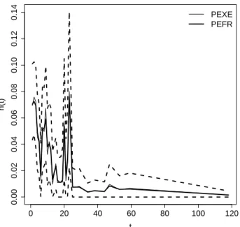
In this section we use the proposed model to analyze the survival times (in months) of 231 individuals diagnosed with brain cancer in Windham-CT, USA, during 1995 to 2004. This data set was obtained from SEER database. Our interest relies on investigate the perfor-mance of our model in estimating both the hazard and survival function. The computational procedures needed to fit the proposed model can be found in Demarqui et al. (2008).

From the 231 patients diagnosed with brain cancer, we observed 134 failures and 97 censored times, resulting in a percentage of failures of the order of 58%. It is also noteworthy that, as the survival times were measured in months, only 32 of the 134 observed failure times correspond to distinct failure times. Thus, under the setup we are proposing, these 32 distinct failure times compose the finest possible time grid for the PEM.

We first examined the performance of the proposed model in estimating the hazard function by comparing the PEFR with the estimates provided by the competing piecewise exponential estimators (PEXE) for the failure rates (Kim and Proschan (1991)), namely, the estimates associated with the nonparametric PEM, obtained via maximum likelihood approach.

0 20 40 60 80 100 120

0.00

0.02

0.04

0.06

0.08

0.10

0.12

0.14

t

h(t)

PEXE PEFR

Figure 1: Estimated hazard function (solid lines) for patients with brain cancer and the 95% HPD interval (dashed lines) provided by the PEM with random time grid.

When there are no ties among the observed survival times, the PEXE for the failure rates are not consistent, once we have only one failure time at each interval, regardless of the sample size n. On the other hand, in the presence of ties, asymptotic results could

intervals for the failure rates should not be computed in these cases. Furthermore, in the finite sample size scenario, little is known theorically about the PEXE (Kim and Proschan (1991)). These drawbacks of the maximum likelihood approach are easily overcome in the setting we are proposing, since HPD intervals do not rely on the sample size n, and can be

obtained straightforwardly.

In Figure 1 we present the PEFR and the PEXE for the failure rates along with the 95% HPD intervals provided by the proposed model. Notice that PEFR and the PEXE for the failure rates are quite similar, and yield essentially the same estimated hazard function for the current data set. From the clinical point of view, the estimated failure rates displayed in Figure 1 indicate a decreasing hazard function, suggesting that the risk of death by brain cancer decreases through time.

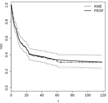
The well known Kaplan-Meyer product limiting estimator (KME) arises as a standard estimator for the survival function. In practice, the PEXE yields a smoothing version of the KME for the survival function. Moreover, as shown in Kitchin et al. (1980), the KME and PEXE for the survival function are asymptotically equivalent. Thus, for the sake of simplicity, we compare the PESF with the KME.

Figure 2 displays the estimated survival functions provided by the PESF and the KME, along with their corresponding 95% confidence and HPD intervals. The similar performance of the two competing estimators in both point and interval estimation for the survival func-tion is also evident.

0 20 40 60 80 100 120

0.0

0.2

0.4

0.6

0.8

1.0

t

S(t)

KME PESF

Figure 2: Estimated survival function (solid lines) for patients with brain cancer and their corresponding 95% confidence and HPD intervals (dashed lines) provided by the PEM with random time grid.

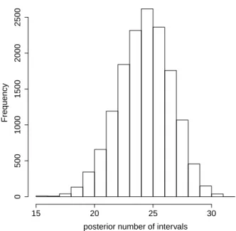
making inferences about the time grid and the number of intervals used to fit the PEM. For instance, the posterior most probable number of intervals is B = 25, with probability 0.174. The estimated 95% HPD intervals for B is [21,29]. Other characteristics of the posterior sample of the number of intervals of the PEM are given in Table 1 and Figure 3.

Table 1: Summary of sample of the posterior distribution of the number of intervals.

mean sd min max

24.779 2.292 15 32

P2

.50 P25.0 P50.0 P75.0 P97.50

20 23 25 26 29

posterior number of intervals

Frequency

15 20 25 30

0

500

1000

1500

2000

2500

4

Conclusions

In this paper we presented a fully Bayesian approach to model time to event data using the piecewise exponential model with random time grid. Extending the previous work due to Demarqui et al. (2008), we elicited noninformative priors for both the time grid and the failure rates. Fixed the time grid, the Jeffreys’ prior for the failure rates is a product distribution favoring the use of the structure of the PPM. It also induces independence among the failure rates in different intervals. Finally, we conducted the analysis of a real data set to illustrate the performance of the proposed model.

The results obtained from the analysis of the brain cancer data set suggest that the estimates provided by the proposed model are comparable with the those yielded by other estimators established in the literature such as the PEXE and the KME. However, interval estimation is straightforward under the framework we are proposing, and it does not rely on asymptotic approximations such as the PEXE and the KME do. Other advantage of the proposed model is that it enriches the analysis by enabling inferences for the time grid of the PEM. Furthermore, the assumption of a joint noninformative prior distribution for the failure rates and the time grids is quite attractive in situations where there is no prior information available.

Acknowledgments

The authors would like to express their gratitude to the editor and the referees for

the careful refereeing of the paper. Fabio N. Demarqui’s research was sponsored by

CAPES(Coordenação de Aperfeiçoamento de Pessoal de Ensino Superior) of the Ministry for

Science and Technology of Brazil. Dipak K. Dey ... Rosangela H. Loschi’s research has been

partially funded by CNPq (Conselho Nacional de Desenvolvimento Científico e Tecnológico)

of the Ministry for Science and Technology of Brazil, grants 306085/2009-7, 304505/2006-4. Enrico A. Colosimo’s research has been partially funded by the CNPq, grants 150472/2008-0 and 306652/2008-0.

References

Aitkin, M., Laird, N., and Francis, B. (1983). A reanalysis of the stanford heart transplant

data (with discussion). J Am Stat Assoc78, 264–292.

Arjas, E. and Gasbarra, D. (1994). Nonparametric bayesian inference from right censored survival data. Stat Sinica 4, 505–524.

Barry, D. and Hartigan, J. A. (1992). Product partition models for change point problems.

Bastos, L. S. and Gamerman, D. (2006). Dynamic survival models with spatial frailty. Lifetime Data Anal 12,441–460.

Breslow, N. E. (1974). Covariance analysis of censored survival data. Biometrics 30,89–99.

Clark, D. E. and Ryan, L. M. (2002). Concurrent prediction of hospital mortality and length of stay from risk factors on admission. Health Services Res 37,631–645.

Demarqui, F. N., Loschi, R. H., and Colosimo, E. A. (2008). Estimating the grid of time-points for the piecewise exponential model. Lifetime Data Anal 14,333–356.

Gamerman, D. (1991). Dynamic bayesian models for survival data. Appl Stat 40, 63–79.

Gamerman, D. (1994). Bayes estimation of the piece-wise exponential distribution. IEEE Trans Reliab 43,128–131.

Ibrahim, J. G., Chen, M. H., and Sinha, D. (2001). Bayesian survival analysis. Springer-Verlag, New York.

Kalbfleisch, J. D. and Prentice, R. L. (1973). Marginal likelihoods based on cox’s regression and life models. Biometrika60, 267–278.

Kim, J. S. and Proschan, F. (1991). Piecewise exponential estimator of the survival function. IEEE Trans Reliab40, 134–139.

Kim, S., Chen, M. H., Dey, D. K., and Gamerman, D. (2006). Bayesian dynamic models for survival data with a cure fraction. Lifetime Data Anal13, 17–35.

Kitchin, J., Langberg, N. A., and Proschan, F. (1980). A new method for estimating life distributions from incomplete data. Technical report, Department of Statistics, Florida State University.

McKeague, I. W. and Tighiouart, M. (2000). Bayesian estimators for conditional hazard functions. Biometrics 56, 1007–1015.

Qiou, Z., Ravishanker, N., and Dey, D. K. (1999). Multivariate survival analysis with positive stable frailties. Biometrics 55, 637–644.

Sahu, S. K., Dey, D. K., Aslanidu, H., and Sinha, D. (1997). A weibull regression model with gamma frailties for multivariate survival data. Lifetime Data Anal 3,123–137.

Sinha,D., Chen, M.H. and Ghosh,S.K.(1999). Bayesian Analysis and Model Selection for Interval-Censored Survival Data. Biometrics55, 585–590.

Flexible Piecewise Exponential Model in Survival

Analysis and Beyond

Fabio N. Demarqui

, Rosangela H. Loschi

,

Enrico A. Colosimo

, Dipak K. Dey

1

_{Universidade Federal de Minas Gerais, Brazil}

2

_{University of Connecticut, USA}

Abstract

In this paper we present semiparametric Bayesian approaches for modeling survival data using the piecewise exponential model (PEM). We assume that the time grid needed to fit the PEM is a random quantity and propose a flexible class of prior dis-tributions for modeling jointly the time grid and its corresponding failure rates. The mechanism used to model the randomness of the time grid of the PEM has several advantages over other approaches that have been proposed in the literature. The resul-tant approach includes other models established in the literature as special cases and provides a flexible framework for survival data modeling. Properties of the model are discussed in the paper. The use of the proposed methodology is exemplified through the analysis of the survival times of patients diagnosed with brain cancer in Windham-CT, USA, obtained from the SEER (Surveillance, Epidemiology and End Results) database. Keywords: Bayesian inference, Gibbs sampler, product partition model, survival anal-ysis.

1

Introduction

also Sinha et al. (1999) for an application to interval-censored data), melanoma, Kim et al. (2006), and nasopharynx cancer, McKeague and Tighiouart (2000), among others. The PEM has also been used in reliability engineering (Kim and Proschan (1991), Gamerman (1994), and Barbosa et al. (1996)), and economics problems, Gamerman (1991), and Bastos and Gamerman (2006).

Let T be a non-negative random variable representing a survival time of interest. In order to construct the PEM, we first need to specify a time grid τ = {s0, s1, ..., sb}, such that 0 = s0 < s1 < s2 < ... < sb < ∞, which induces a partition of the time axis into b

intervals Ij = (sj−1, sj], for j = 1, ..., b. Then, we assume a constant failure rate for each

interval induced by τ, that is:

h(t) = λj, t∈Ij, j = 1,· · · , b.

In order to express the cumulative hazard, the survival and the density functions, we define:

tj =

    

sj−1, if t < sj−1,

t, if t∈Ij,

sj, if t > sj,

(1)

for j = 1, ..., b.

The cumulative hazard function of the PEM is computed from (1), yielding:

H(t|λ_{, τ) =} b

∑

j=1

λj(tj−sj−1). (2)

It follows from the well-knwon identity S(t) = exp{−H(t)}that the survival function of the PEM is given by:

S(t|λ, τ) = exp

{

− b

∑

j=1

λj(tj−sj−1)

}

. (3)

The density function associated withT is obtained by taking minus the derivative of (3). Thus, we say that the random variable T follows a PEM with time grid τ and vector of parameter λ_{= (λ1, ..., λb)}′_{, denoted byT ∼P ED(τ,λ), if its probability density function is}

given by:

f(t|λ, τ) =λjexp

{

− b

∑

j=1

λj(tj −sj−1)

}

, (4)

for t∈Ij and λj >0, j = 1, ..., b.

The time grid τ ={s0, s1, ..., sJ} plays a central role in the goodness of fit of the PEM.

rates, whereas a time grid based on just a few intervals might produce a poor approximation for the true survival function. In practice, we desire a time grid which provides a balance between good approximations for both the hazard and survival functions. This issue has been one of the greatest challenges of working with the PEM. Although the PEM has been widely used in the literature, the time grid τ ={s0, s1, ..., sb}has been arbitrarily chosen in

most of those works. Kalbfleisch and Prentice (1973) suggested that the selection of the time grid τ = {s0, s1, ..., s_b} should be made independent of the data, but they did not provide any procedure to do such. Breslow (1974) proposed defining the endpointssj of the intervals

Ij as all the observed failure times. We shall refer the PEM constructed based on such time

grid to as nonparametric PEM. Other heuristic discussions regarding adequate choices for the time grid of the PEM can be found in Gamerman (1991), Sahu et al. (1997) and Qiou et al. (1999), to cite few.

In practice, the problem of specifying a suitable time grid to fit the PEM can be overcome by assuming that τ = {s0, s1, ..., sb} is itself a random quantity to be estimated using the

data information. The first effective effort in this direction is due to Arjas and Gasbarra (1994). In that work it is assumed that the endpoints of the intervalsIj are defined according

to a jump process following a martingale structure which is included into the model through the prior distributions. Similar approaches for modeling the time grid of the PEM were considered by McKeague and Tighiouart (2000) in the context of regression models and Kim et al. (2006) to fit cure rate models. Independently from those works, Demarqui et al. (2008) also proposed an approach which considers a random grid for the PEM. Based on the usual assumptions for the time grid and assuming independent Gamma prior distributions for the failure rates, they proved that the prior distribution for the time grid has a product form, and have used the structure of the Product Partition Model (PPM) proposed by Barry and Hartigan (1992) to handle the problem. By considering such approach, the the reversible jump algorithm can be used to sample from the posterior distributions of interest.

In this paper we introduce a general framework for modeling survival data using the PEM via PPM. The proposed methodology offers more flexibility in fitting the PEM by allowing a broad class of prior distributions for(λ_{, τ). The resultant model includes as special cases the}

models proposed by Demarqui et al. (2008), Gamerman (1994) and Ibrahim et al. (2001a), and any other model whose prior process satisfies the (conditional) independence condition for the failure rates and yields a closed form expression for the marginal distribution of the data. Finally, we illustrate the usefulness of the proposed methodology by analyzing the survival times of patients diagnosed with brain cancer in Windham-CT, USA, obtained from the SEER (Surveillance, Epidemiology and End Results) database. The results obtained by using our approach are compared with those provided by other methods existing in the literature.

Section 4 some conclusions are drawn about the proposed model.

2

A general class for the PEM via PPM

In the following sequence, we formally introduce the general framework for fitting the PEM via PPM. The notation, as well as the conditions under which our new methodology relies on, are addressed in Section 2.1. Particular cases arising from objective and subjective prior specifications for the failure rates of the PEM are properly discussed in Sections 2.2 and 2.3, respectively.

2.1

Model formulation

We start our model formulation by assuming that only time grids whose endpoints are equal to distinct observed failure times are possible. This mild constrain on the set of possible time grids can be justified by the plausible argument that the observed failure times are themselves good candidates for the endpoints of the intervals needed to fit the PEM. In addition, such constrain also guarantees the existence of at least one failure time at each interval induced by the random time grid of the PEM.

Formally speaking, let F _{= {0, y1, ..., ym} be the set formed by the origin and the m}

distinct ordered observed failure times from a sample of size n. Consider the time grid

τ′ _{= {0, y}′

1, ..., ym′ ′} satisfying τ′ ⊆ F, where m′, 1 ≤ m′ ≤ m, denotes the maximum

number of intervals admitted a priori. Then, the time grid τ′ _{= {0, y}′

1, ..., ym′ ′} induces the

following set of disjoint intervals:

Ij = {

(0, y′

1], if j = 1, (y′

j−1, yj′], 1< j ≤m′.

(5)

Further, denote by I ={1, ..., m′_{} the set of indexes related to the intervals defined in (5).}

Let ρ = {i0, i1, ..., ib}, 0 = i0 < i1 < ... < ib = m′, be a random partition of I dividing the

m′ _{initial intervals given in (5) intoB =b new disjoint intervals, where the random variable}

B denotes the number of clustered intervals related to the random partition ρ. Finally, let

τ =τ(ρ) = {s₀, s₁, ..., sb} be the time grid induced by the random partitionρ, where

sj = {

0, if j = 0, y′

ij, if j = 1, . . . , b,

(6)

for b = 1, ..., m′_{. Hence, it follows from (5) and (6) that the clustered intervals induced by} ρ={i0, i1, ..., ib}are given by:

I_ρ(j) =∪ij

Then, givenρ={i0, i1, ..., ib}, we assume that:

h(t) = λr ≡λ(ρj), (8)

whereλ(ρj) denotes the common failure rate associated with the clustered intervalIρ(j),ij₋1 <

r ≤ij, r= 1, ..., m′ _{and j = 1, ..., b.}

In order to properly construct the likelihood function over the b intervals induced by

τ(ρ) ={s0, s1, ..., sb}, we redefine (1) in order to accommodate accordingly the information

of the n elements belonging to the observed sample as:

tij =   

 

sj₋1, if ti < sj−1,

ti, if ti ∈Iρ(j), sj, if ti > sj,

(9)

for j = 1, ..., b and i= 1, ..., n. Further, we also defineδij =δiν_j(i), where ν_j(i) is the indicator function assuming value 1 if the survival time of the i-th element falls in the j-th interval, and 0 otherwise.

Due to the one-to-one relationship betweenτ andρ, it is possible to express the likelihood function in terms of the random partitionρ. Then, under the assumption that there is a right-censoring scheme working independently of the failure process it follows that the contribution of a survival time (either failure or censored) ti ∈Iρ(j) for the likelihood function of the PEM

reduces to ∏b j=1(λ

(j)

ρ )δijexp{−λ(ρj)(tij −sj₋1)}. Thus, the entire likelihood function can be

written as:

L(λ_{ρ, ρ|D) =} n ∏

i=1

( _b ∏

j=1

(λ(ρj))

δij_exp{_−λ(j)

ρ (tij −sj−1)

} )

= b ∏

j=1

(λ(j)

ρ )

ηj_exp{ −λ(j)

ρ ξj }

, (10)

where the number of failures, ηj =∑n

l=1δij, and the total time under test observed at each

interval Iρ(j), ξj =∑_in₌₁(tij −sj₋1), are sufficient statistics for λ(

j)

ρ ,j = 1, ..., b.

The joint prior distribution for (λ_{ρ, ρ) is specified hierarchically by first eliciting a prior}

distribution for the random partition ρ, and then specifying a prior distribution for λ_ρ,

conditionally on ρ, that is,

π(λ_{ρ, ρ) =π(}λ_{ρ|ρ)π(ρ). (11)}

can be written as the product form:

π(ρ={i₀, i₁, ..., ib})∝ b

∏

i=1 c

Iρ(j), (12)

for 0 = i0 < i1 < ... < ib = m′ and b ∈ I. Here, c_I(j)

ρ , called prior cohesion, is a positive

quantity representing the degree of similarity among the intervals being clustered. Moreover, accordingly normalized, the prior cohesionsc_I(j)

ρ can be interpreted as the one-step transition

probability of the Markov Chain defined by the endpoints of the clustered intervals Iρ(j),

j = 1, ..., b.

We further assume that, conditionally on ρ, the joint prior distribution for λ_{ρ can be}

expressed by the following product form:

π(λ_{ρ|ρ) =}

b

∏

j=1 π(λj

ρ). (13)

This assumption is equivalent to assume that, for a given ρ, the common failure rates are independent a priori. Hence, conditionally onρ, it follows from (10) and (13) that the joint (marginal) distribution of the observations reduces to the product form:

f(D|ρ) =

b

∏

j=1 ∫

(

λ(_ρj))ηjexp{

−ξjλ(ρj)

} π(λ(j)

ρ )dλ(ρj). (14)

According to Barry and Hartigan (1992), any joint distribution of the observations and partitions that satisfies the product condition for the partitions and the independence tion for observations, given the partition, follows a PPM. Consequently, the product condi-tion follows for the joint distribucondi-tion of the observacondi-tions given in (14), provided the integrals are well defined (where we mean by well defined finite intervals), and the clustering structure of the PPM can be extended for modeling the randomness of the time grid of the PEM.

The joint posterior distribution of(λ_{ρ, ρ) is:}

π(λ_{ρ, ρ|D) ∝ L(}λ_{ρ, ρ|D)π(}λ_ρ|ρ)π(ρ)

≡ π(λ_{ρ|ρ,D)π(ρ|D). (15)}

Then, it follows from (12) and (13) that the posterior distribution of the random partition

ρ is given by:

π(ρ|D) ∝ f(D|ρ)π(ρ)

∝ b

∏

i=1 c∗

Iρ(j)

where c∗

Iρ(j)

= (∫ λ(ρj)(λ

(j)

ρ )νjexp {

−λ(ρj)ξj }

π(λ(ρj))dλ(ρj) )

c

Iρ(j) denotes the posterior cohesion

associated with j-th clustering interval Iρ(j).

Following the structure of the PPM, we have that the posterior distribution ofλkis given by the following mixture of distributions:

π(λk|D) = ∑

ij−1<k≤ij

π(λ(_ρj)|D, ρ)R(I_ρ(j)|D), (17)

fork = 1, ..., m′_{, whereR}

(Iρ(j)|D)is named as posterior relevance, and denotes the probability of each clustered interval Iρ(j) to belong to the random partition ρ, and π(λ(ρj)|D, ρ)denotes the full conditional posterior distribution of the common parameter λ(ρj), j = 1, ..., b.

Then, assuming the squared-error loss function, it follows that the product estimate for the failure rate (PEFR) λk is given by:

ˆ

λk= ∑

ij−1<k≤ij

E(λ(_ρj)|D, ρ)R(I_ρ(j)|D), (18)

for j = 1, ..., band k= 1, ..., m′_.

Under this structure, the posterior survival function for a new element, assumed to be independent of the observed data set, is obtained by averaging the conditional survival function S(y|D, ρ) over all random partitionsρ={i0, i1, ..., ib}, that is:

S(y|_D) = ∑ ρ

S(y|_D, ρ)π(ρ|_D), (19)

where

S(y|_D, ρ) = ∫

S(y|λ_{ρ, ρ)π(}λ_{ρ|D, ρ)d}λ_ρ,

(20)

forλ_{ρ = (λ}(1)_{ρ , ..., λ}(_ρb)₎′_{. Throughout this paper we shall refer to (20) as product estimate for}

the survival function (PESF).

2.2

Objective prior elicitation

A full objective analysis can be performed by assuming the Bayes-Laplace prior distribution for ρ, and, the Jeffreys prior distribution for λ_{ρ, givenρ.}

The Bayes-Laplace prior distribution for ρ corresponds to the special case of the prior distribution (12) in which c_I(j)

ρ = 1, ∀ j such that (ij−1, ij) ∈ I. Now, given ρ, let I( λ_ρ)

λ_{ρ is defined as:}

π(λ_{ρ|ρ) ∝ |I(}λ_ρ)|12

∝ b

∏

j=1

(

λ(_ρj))−1

. (21)

An attractive characteristic of the Jeffreys prior is that it is invariant under param-eterizations, a desired feature of objective prior distributions. Moreover, it also induces independence among the λ(ρj)’s. Thus, the product condition required to use the structure of the PPM to model the PEM with random time grid is satisfyied.

It follows from (12) and (21) that the joint prior distribution for (λ_{ρ, ρ)is given by:}

π(λ_{ρ, ρ) ∝}

b

∏

j=1

(

λ(_ρj))−1, (22)

which is an improper prior distribution.

Replacing (22) in (15), the joint posterior distribution of (λ_{ρ, ρ) becomes:}

π(λ_{ρ, ρ|D)∝}

b

∏

j=1

(

λ(_ρj))νj−1

exp{

−ξjλ(ρj)

}

, (23)

which is a proper posterior distribution. This is a direct consequence of our model formu-lation, which ensures that both νj >0 and ξj >0, ∀ j = 1, ..., b, regardless ofρ. Moreover, after a simple algebra, the posterior distribution of ρ in (16) becomes:

π(ρ|D)∝ b

∏

j= Γ(νj)

ξηj j

,

where Γ(·)denotes the gamma function.

2.3

Subjective prior elicitation

The gamma family of distributions has been widely used as prior distributions for the fail-ure rates of the PEM. This family of distributions corresponds to the conjugate family of prior distributions for the exponential sample family, and facilitates the inference processs regarding the PEM. In addition, structures of dependence between successive intervals can be easily introduced through its hyper-parameters (Arjas and Gasbarra (1994), Gamerman (1994) and Ibrahim et al. (2001a), among others).

2.3.1 Independent priors

Assume that the components of λ_{ρare conditionally independent, with each λ}(_ρj) _{following a} gamma distribution with shape and scale parameters αj andγj, respectively, forj = 1, ..., b.

Then, considering (12), the joint prior distribution for (λ_{ρ, ρ) becomes:}

π(λ_{ρ, ρ) ∝}

b

∏

j=1

( λ(j)

ρ

)αj−1 exp{

−γjλ(ρj)

} c_I(j)

ρ . (24)

In the case that information regarding the mean of the failure rates and their variances is available, informative prior distributions for the λ(ρj)’s can be obtained by solving the system

of equations formed by E(λ(ρj)) = αj/γj and V(λ

(j)

ρ ) = αj/γj2. Furthermore, by replacing

(24) in (15), the posterior distribution of (λ_{ρ, ρ) becomes:}

π(λ_{ρ, ρ|D)∝}

b

∏

j=1

γαj

j

Γ(αj)

( λ(j)

ρ

)αj+ηj−1 exp{

−[γj+ξj]λ(ρj)

} c_I(j)

ρ . (25)

It is straightforward to show that the posterior distribution for the random partition ρ given in (16) reduces to:

π(ρ|D)∝

b

∏

j=

γαj

j

Γ(αj)

Γ(αj +ηj)

(γj+ξj)αj+ηj

c_I(j) ρ ,

and, not surprisingly, (λ(ρj)|D, ρ)∼Ga(αj+ηj, γj +ξj), for all j = 1, ..., b.

Although the gamma family of distributions allows for subjective elicitation of the prior distribution of each common failure rate λ(ρj), due to the randomness of ρ, it is not possible,

in practice, to set a "realistic" informative prior distribution for each component of λ_{ρ by} a direct specification of the hyper-parameters αj and γj. In this fashion, in the original

formulation of the PEM via PPM, Demarqui et al. (2008) assumed that the common fail-ure rates were i.i.d. with λ(ρj) ∼ Ga(α0, γ0), ∀ j = 1, ..., b. Nevertheless, considering this

specification, the prior means indicate a constant hazard function through time (equals to α0/γ0), which may not be in accordance with a gamma of hazard functions associated with

many applications. Therefore, this drawback turns necessary the search for more compre-hensive mechanism for the prior elicitation of λρ. In the next two subsections we discuss two

approaches which overcome this drawback.

2.3.2 Dynamic priors

a special case when we set P(ρ={i0, i1, ..., ib}) = 1 for a particular partition.

LetD(0)ρ be the subjective information that we have before the data has been observed.

Denote by Dρ(j) the set of all information gathered up to the j-th clustered interval Iρ(j),

j = 1, ..., b. We perform the following sequential analysis: i) Setj = 1, and specify (λ(ρj)|Dρ(j−1), ρ)∼Ga(αj;γj);

ii) Update the prior available information contained in (λ(ρj)|Dρ(j−1), ρ) with the data

in-formation provided by Iρ(j), yielding(λ(ρj)|Dρ(j), ρ)∼Ga(αj +ηj;γj+ξj);

iii) Perform the parametric evolution (through time) by setting(λ(ρj+1)|Dρ(j), ρ)∼Ga(αj+1;γj+1),

where αj+1 = (αj +ηj)φ and γj+1 = (γj+ξj)φ, with 0< φ≤1;

iv) Increment j, return to step (ii), and repeat the cicle until all data information has been processed.

In the literature of dynamic models, the complete conditional posterior distribution

(λ(ρj)|Dρ(j), ρ) is often referred to as online distribution. The quantity φ, called discount

factor, controls the passage of information through successive intervals. As closer to one is

φ, as much information is allowed to pass from one interval to another. On the other hand, as φ →0, no information passes to the next interval, providing b independent estimations. Moreover, by setting (λ(ρj)|Dρ(j−1), ρ) ∼ Ga([αj−1 +ηj−1]φ; [γj−1 +ξj−1]φ), we have a prior

distribution forλ(ρj) which has the same mean of(λρ(j−1)|Dρ(j−1), ρ), but with a variance larger

than V(λ(j−1),ρ

ρ |D(ρj−1), ρ).

The dependence between λ(ρj)’s associated with adjacent clustered intervals is specified

through the hyper-parameters of their corresponding prior distributions. In this fashion, the components of λ_{ρ are conditionally independent, and, consequently, the joint prior}

distribu-tion for (λ_{ρ, ρ) can be written in the product form given in (24). Therefore, the conditions}

stated earlier in this text to model the randomness of the time grid of the PEM still hold in the present case.

The sequential analysis described above is equivalent to assume that the common failure rates λ(ρj)’s are related via the following evolution equation:

log(λ(j)

ρ ) = log(λ

(j−1)

ρ ) +εj, (26)

where εj is a stochastic error with mean zero and variance given by:

σ2_j =

(

1

φ −1

)

V[log(λ(j−1) ρ )|D

(j−1)

ρ , ρ].

From equation (26) it is possible to obtain the complete conditional posterior distributions of each common failure rateλ(ρj)given all the available information contained inDρ(b), denoted

more informative than the online distributions (λ(ρj)|D(ρj))’s, which are based only upon the information available up to the current intervalIρ(j), and therefore, should be preferred when making inferences for the components of λ_{ρ. The recursive (smoothing) algorithm used to} obtain the smoothed distributions (λ(ρj)|Dρ(b), ρ)’s can be found in Gamerman (1991).

2.3.3 Structural priors

In this section we consider the structural (hierarchical) framework, first introduced by Ibrahim et al. (2001a) in the context of cure rate models, to set a prior distribution for λρ. We refer such approach to as structural because the prior distribution for the λ(ρj)’s are built under the assumption that both their means and variances are functions of a cumu-lative hazard function associated with a parametric distribution. Such structural modeling approach is particularly suitable for situations in which the estimation of the right tail sur-vival curve is affected by the lack of data information.

Assume that the components of λ_{ρ are independent a priori so that each λ}(_ρj) _{has a} Gamma prior distribution with mean and variance, respectively, given by:

µj =E(λ(ρj)|λ0, κ) =

H0(sj)−H0(sj−1)

sj −sj−1

(27)

and

σ2_j =V(λ(j)

ρ |λ0, κ) = µjκj, (28)

whereH0(·|λ0)is a cumulative hazard function of a parametric survival distributionF0(·|λ0).

The choice ofF0(·|λ0)is arbitrary and must reflect someone’s opinion about the right tail

of the survival curve. Note that, by taking κ→ 0, the prior process approaches h0(t|λ0) =

d

dyH0(t|λ0), once σ

2

j → 0 and we have that h0(t|λ0)≈

H0(sj)−H0(sj−1)

sj−sj−1

, for t ∈Ij = (sj−1, sj],

j = 1, ..., b. Therefore, κ controls the degree of parametricity along the time axis. In particular, when j → ∞, the right tail of the survival curve converges to the parametric model F₀(·|λ₀), regardless of the value assumed for κ (Ibrahim et al. (2001a)).

Considering the third parameter λ₀ (possible vector valued), the posterior distribution given in (15) becomes:

π(λ_ρ, λ₀, ρ|D) ∝ L(λ_ρ, ρ|D)π(λ_ρ|λ₀, ρ)π(ρ)π(λ₀)

≡ π(λ_{ρ|λ0, ρ,D)π(λ0, ρ|D),}

use the following complete conditional posteriors distributions:

π(ρ|λ0,D)∝ b

∏

j=1

(

(1/κj₎µjκ−j

Γ(µjκ−j)

Γ(µjκ−j +ηj)

(κ−j_+ξ j)µjκ

−j_+ηj

)

c(j)ρ (29)

and

π(λ0|ρ,D)∝

( _b ∏

j=1

(1/κj₎µjκ−j

Γ(µjκ−j)

Γ(µjκ−j+ηj)

(κ−j _+ξ j)µjκ−

j_+ηj

)

π(λ0). (30)

The similarity between the complete conditional posterior distributions given in (26) and (29) is evident, since the second one depends on λ0 only through the µj’s. Therefore, the

Gibbs sampling algorithm proposed by Barry and Hartigan (1993) can still be used to sample from (29).

We emphasize here that, although that structural modeling approach has been considered before by Ibrahim et al. (2001a), an approach considering simultaneously that hierarchical structure along with a random time grid for the PEM have not been considered in the literature yet.

3

Analysis of real data set

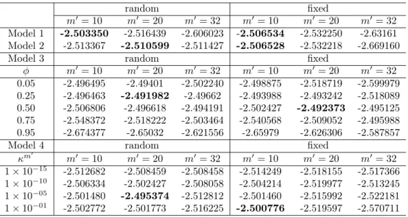
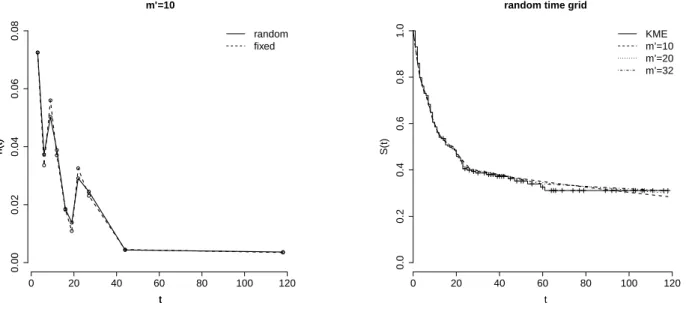
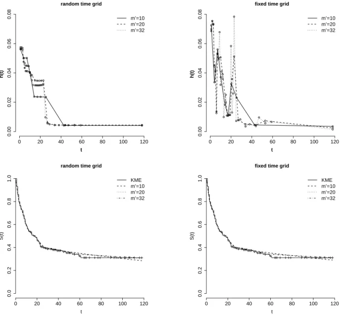
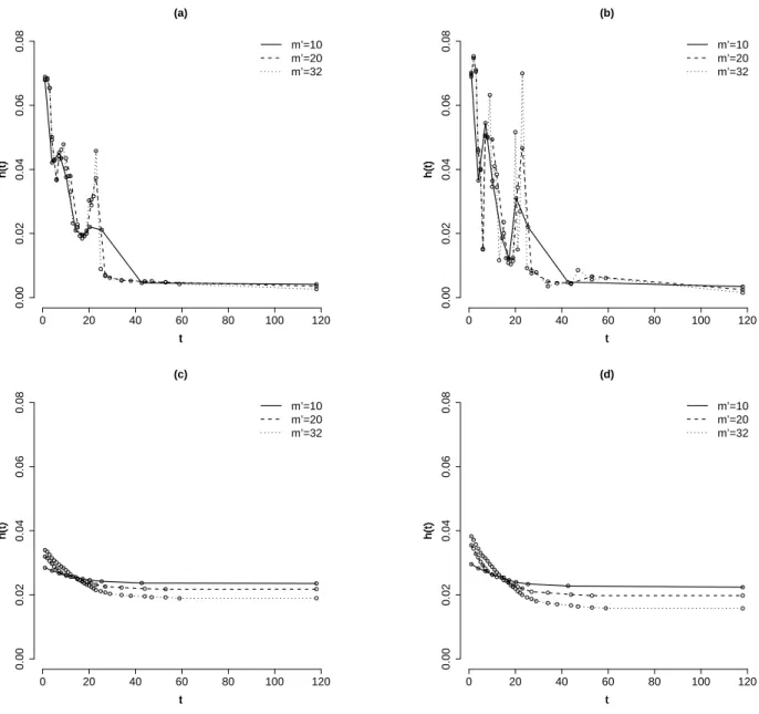
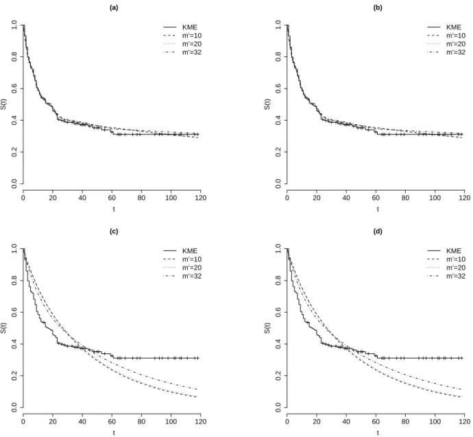
We use the proposed methodology in this section to analyze the survival times (in months) of 231 individuals diagnosed with brain cancer in Windham-CT, USA, during 1995 to 2004. This data set was obtained from SEER database. Our interest here relies on investigate the performance of the models discussed in the previous sections in estimating both the hazard and survival function. We further carry out a sensitivity analysis taking into account different specifications for m′_{, φ and κ as well.}

From the 231 patients diagnosed with brain cancer in this period, it was observed 134 deaths and 97 censored times, resulting in a percentage of failures of the order of 58%. It is also noteworthy that, since the survival times were measured in months, only 32 of the 134 observed failure times were distinct failure times. In order to set the finest time grid for the PEM we proceed as follows. Given m′_{, we obtain k and r such that m =km}′_{+r. The}

elements of τ′ _{are then chosen so that the first m}′_{−r intervals havek failure times and the}

remainingr intervals havek+ 1failure times. We note that this procedure for specifying the finest time grid assumed for the PEM is appealing in the sense that it allows more failure times to be placed in the last intervals, where less data information is available.

In the following analysis, we will restrict our attention to discrete uniform prior distri-butions for the random partition ρ. Such prior distributions can be obtained by setting

c_I(j)

ρ = 1 for all j = 1, ..., b, b∈ I. Other prior specifications for the random partition ρ, can

Jeffreys prior distribution for λρ introduced in Section 2.2. The model originally proposed

by Demarqui et al. (2008), briefly discussed in Section 2.3, is referred to as Model 2. For that specific model, it is assumed that λ(ρj) ∼Ga(0.001; 0.001) for all j = 1, ..., b, and b ∈ I,

so that the λ(ρj)’s have a flat prior distribution with mean 1 and variance equals to 1000.

The dynamic model described in Section 2.3.2 is referred to as Model 3. For that case, we assume that (λ(1)ρ |D(0)ρ )∼Ga(0.001; 0.001). Finally, Model 4 is referred to as the structural

model discussed in Section 2.3.3. For that model the Weibull distribution with cumulative hazard function H(t|λ0) = exp(β)tζ, where λ0 = (ζ, β)′ was considered. Consequently, it

follows that µj = exp(β)(sζj −s ζ

j−1)/(sj −sj−1) and σ2j = κjexp(β)(s ζ j −s

ζ

j−1)/(sj −sj−1).

In this case, we assumed that ζ and β are independent a priori, with ζ ∼Ga(0.001; 0.001)

and β ∼N(0; 1000), respectively.

Samples from the quantities of interest were obtained by using MCMC techniques. Specif-ically, the Gibbs sampler algorithm proposed by Barry and Hartigan (1993) was considered to sample from the posterior distribution of the random partition ρ, and the adaptive rejec-tion Metropolis sampling (ARMS) algorithm introduced by Gilks et al. (1995) was used to sample from the posterior distribution of λ0 = (ζ, β)′, whereas samples from the posterior

distribution of λρwere obtained straightforwardly. For all scenarios considered in our

analy-sis, it was considered single chains of size 100,000. Samples of size 1,000 were obtained after considering a burn-in period of 50,000 iterations and a lag of 50 to eliminate correlations. All computational procedures were implemented in the Object-oriented Matrix Program-ming Language Ox version 5.1 (Doornik; 2007), and are available from the first author upon request.

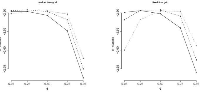
In order to evaluate the performance of the models under investigation, we considered the average of the logarithm of the pseudo-marginal likelihood as a measure to assess the goodness of fit of each model. Such measure, which we shall refer to as B-statistic, is based on the conditional predictive ordinate (CPO) statistic (see Ibrahim et al. (2001b) and references therein), and is defined as

B = 1

n

n

∑

i=1

log(CP Oi). (31)

Here, the quantityCP Oi corresponds to the posterior predictive density ofti ifti is a failure

time, and the posterior predictive probability of the event (T > ti) if ti is a censored time.

In both cases, it can be shown that the CP Oi can be well approximated by

[

CP Oi =M

{ _M

∑

l=1

[L(ti|λlρl, ρl)]−1 }−1

, (32)

where (λl

ρl, ρl) corresponds to the l-th draw of the the posterior distribution π(λ_ρ, ρ|D),