Abstract—In this paper a detailed description and analysis of the time domain Frequency-Dependent Bergeron’s method is presented. In order to include the frequency dependence into a time domain based model, the frequency effect in the longitudinal parameters is performed through the approximation of the Z(ω)by a rational function using vector fitting. This function is modeled by discrete elements of electrical circuits obtained through the poles and zeros of the adjusted Z(ω) curve. Thus, the frequency effect can be included in the Bergeron’s model directly in the time domain. The model can be used to simulate electromagnetic transients with a response similar to the prestigious Universal Line Model and similar to the frequency-dependent cascade of π circuits.
Index Terms—Transmission line matrix methods. Frequency estimation. Electromagnetical transients. Time-domain analysis.
I. INTRODUCTION
N general terms, power transmission systems can be modeled as a set of dynamic systems bounded to initial conditions and boundary conditions. Thus, the continuous improvement and creation of new computational tools to simulate more efficiently those dynamic systems is not outdated [1].
Initially, a brief review of the state of art on Transmission Line Modeling – TLM is described emphasizing the advantages and the main problems in the area.
Several Transmission line models are available in the literature. Most of them may be classified in two categories: by distributed parameters and by lumped parameters.
The line modeling by distributed parameters is developed directly from the frequency-dependent parameters of the transmission line, where the differential equations are proposed and solved by means of inverse transforms and convolutions to obtain a time domain representation of the variables of interest [1]. One of the main limitations of the frequency domain models solved in the frequency domain is that the representation of nonlinear elements isn’t always possible nor simple.
In the second category, a line is represented by an interaction of lumped elements, i.e., the line is represented by an equivalent interaction of its traditional circuit elements: resistance, inductance and capacitance lumped into one or more specific points along the section. Most of
This research was supported by Fundação de Amparo à Pesquisa do Estado de São Paulo-FAPESP
these models are directly developed in the time domain. The representation of nonlinear elements is one of the main advantages of using time domain techniques to represent transmission lines [2]. The frequency effect on the longitudinal parameters can be included in the line modeling using fitting methods [3].
The Bergeron method, also known as method of the characteristics, was applied to solve electrical problems, more specifically, electromagnetic wave propagation along a lossless line [4], leaving only longitudinal inductance L and the shunt capacitance C. Thereafter Dommel, in order to approximate line loses, combined the Bergeron method with lumped frequency-fixed resistances. This model was the first practical mathematical model addressing computational modeling of transmission lines.
Subsequently, Dommel proposed a nodal solution combining the method of characteristics for transmission lines and the trapezoidal rule of integration for the lumped parameters. From this development, the electromagnetic transient program – EMTP was created and a new line model for lossless transmission lines was proposed [5].
In reference [6], an extension of the Bergeron’s method
of characteristic was developed including line’s loses and the
frequency effect on the longitudinal parameters by means of inverse transforms. The main contribution of Snelson, in reference [6] is the inclusion of the line losses in the Bergeron model using lumped resistances at both line terminals, concentrating the line losses at the sending and receiving ends of the line section.
New frequency-dependent models by lumped parameters have been recently published in the technical literature on power system modeling. These models are developed directly in the time domain, representing the line as a
cascade of π-circuits, where frequency dependent longitudinal impedance is modeled as an arrangement of resistances Rfit and inductances Lfit. These parameters are based on the longitudinal impedance of the line, Z(ω), calculated taking into account the earth-return impedance (soil effect) and the skin effect on the cables along a wide frequency range. The resulting system is solved as a linear system through one of the many integration methods available. The model described in [7] shows to be robust and accurate for the most of transient conditions on a conventional power transmission system. However, the
Using the Frequency-Dependent Bergeron Line
Model to Simulate Transients
Pablo Torrez Caballero, Eduardo C. Marques Costa and Sergio Kurokawa
model shows to be costly in computational terms as the size of the problem to be solved increases with the quantity of line equivalent segments, the total simulation time and the number of arrangements of resistances and inductances.
Based on the contributions firstly proposed by Dommel and after by Snelson, the current research proposes the use of a new line model that takes into account the frequency dependence of the longitudinal parameters into the Bergeron line model, maintaining its characteristic robustness and simplified modeling. Taking advantage of this model, the main contribution of this research is the implementation of the frequency-dependent Bergeron Line Model.
The combination of the Bergeron line model and the inclusion of the frequency dependence results in an accurate line model capable to simulate electromagnetic transients composed of a wide range of frequencies, emphasizing that most of line models in the time domain have restrictions for simulations including a wide range of frequencies [1].
This paper is structured into three parts. The first part is an introduction of the classical Bergeron model for lossless lines and for lossy lines using constant parameters. The second part describes the inclusion of the frequency effect on the Bergeron line model using vector fitting. The third part shows the implementation of the model and compares its output with two well-established line models: a frequency-domain model using numerical Laplace transform [1] and a frequency-dependent cascade of π circuits [3] [7].
II. THEBERGERONLINEMODEL
The Bergeron line model was first applied to transmission lossless lines, where resistance R and conductance G were neglected. The remaining parameters: inductance L and capacitance C were fixed in the frequency and solved using the method of characteristics. Considering a single-phase line with length l, the current and voltage at a point x along the line are related by the following differential equations:
𝜕 𝑖(𝑥, 𝑡)
𝜕𝑥 = −𝐶′
𝜕 𝑉(𝑥, 𝑡)
𝜕𝑡 (1)
𝜕 𝑉(𝑥, 𝑡)
𝜕𝑥 = −𝐿′
𝜕 𝑖(𝑥, 𝑡) 𝜕𝑡
(2)
Where the right portion of (1) and (2) represents the voltage and current variations along 𝑥, the other portion represent variations through the time 𝑡.
The general solution of (1) and (2) is expressed [5]: 𝑖(𝑥, 𝑡) = 𝑓1(𝑥 − 𝑣𝑡) + 𝑓2(𝑥 + 𝑣𝑡) (3)
𝑉(𝑥, 𝑡) = 𝑍𝑓1(𝑥 − 𝑣𝑡) − 𝑍𝑓2(𝑥 + 𝑣𝑡) (4)
Where 𝑓1 and 𝑓2 are arbitrary functions of (𝑥 ± 𝑣𝑡), they can be seen as wave propagation functions. 𝑓1 represents the forward traveling wave and 𝑓2 represents the backward traveling wave. Both waves travel with velocity 𝑣 (known as propagation velocity). Terms 𝑍 and 𝑣 are expressed as follow:
𝑍 = √𝐶′𝐿′ (5)
𝑣 = 1
√𝐿𝐶 (6)
Multiplying (3) by the characteristic impedance 𝑍, adding and subtracting it from (4) we obtain (7) and (8) [4]:
𝑉(𝑥, 𝑡) + 𝑍 𝑖(𝑥, 𝑡) = 2𝑍𝑓1(𝑥 − 𝑣𝑡) (7)
𝑉(𝑥, 𝑡) − 𝑍 𝑖(𝑥, 𝑡) = −2𝑍𝑓2(𝑥 + 𝑣𝑡) (8)
Analyzing (7) and (8), 𝑉 + 𝑍𝑖 is constant when (𝑥 − 𝑣𝑡) is constant. Similarly, 𝑉 − 𝑍𝑖 is constant when (𝑥 + 𝑣𝑡) is constant.
Since the velocity 𝑣 is constant and the sending and receiving terminal of the line are fixed points in the space, the propagation time of the wave is defined as follows:
𝜏 =𝑑
𝑣 = 𝑑√𝐿𝐶 (9)
The forward wave is constant from one terminal to the other terminal of the line at instant 𝑡 − 𝜏. From this analysis, the following expression is given:
𝑉𝑚(𝑡 − 𝜏) + 𝑍 𝑖𝑚,𝑘(𝑡 − 𝜏)
= 𝑉𝑘(𝑡) + 𝑍 (− 𝑖𝑘,𝑚(𝑡)) (10)
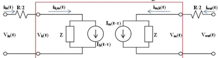
From (10), the equivalent circuit for a lossless line is described in Fig. 1.
Fig. 1. Equivalent impedance circuit of the Bergeron Line Model
By association from (10) and the two-port system showed in Fig. 1, the historical current 𝐼𝑘 and 𝐼𝑚 are [5]:
𝐼𝑘(𝑡 − 𝜏) = −1𝑍 𝑉𝑚(𝑡 − 𝜏) − 𝑖𝑚,𝑘(𝑡 − 𝜏) (11)
𝐼𝑚(𝑡 − 𝜏) = −1𝑍 𝑉𝑘(𝑡 − 𝜏) − 𝑖𝑘,𝑚(𝑡 − 𝜏) (12)
Analyzing the electrical circuits in Fig. 1, the currents 𝑖𝑘,𝑚 and 𝑖𝑚,𝑘 are calculated as follow:
𝑖𝑘,𝑚(𝑡) =1𝑍 𝑉𝑘(𝑡) + 𝐼𝑘(𝑡 − 𝜏) (13)
𝑖𝑚,𝑘(𝑡) =1𝑍 𝑉𝑚(𝑡) + 𝐼𝑚(𝑡 − 𝜏) (14)
Equations (11)-(14) are the time-domain formulation for a lossless line represented by the equivalent impedance circuit described in Fig. 1.
Dommel approximated the losses concentrating the losses at both terminals of the line as shown in Fig. 2.
Fig. 2. Equivalent impedance circuit considering the line losses
𝑖𝑖𝑛(𝑡) =𝑍 1
𝑚𝑜𝑑𝑖𝑓𝑖𝑒𝑑𝑉𝑘(𝑡) + 𝐼𝑘(𝑡 − 𝜏) (15)
𝑖𝑜𝑢𝑡(𝑡) =𝑍 1
𝑚𝑜𝑑𝑖𝑓𝑖𝑒𝑑𝑉𝑚(𝑡) + 𝐼𝑚(𝑡 − 𝜏) (16)
Where 𝑍𝑚𝑜𝑑𝑖𝑓𝑖𝑒𝑑 is the input impedance seen in the sending terminal of the system and the currents 𝐼𝑘 and 𝐼𝑚 are function of the historical combination of voltages and currents in another points in the circuit.
If 𝑛 = 1 as shown in Fig. 2, the following impedance and currents are used in (15) and (16):
𝑍𝑚𝑜𝑑𝑖𝑓𝑖𝑒𝑑 = 𝑍 +𝑅2 (17)
𝐼𝑘(𝑡 − 𝜏) = −𝑍 1
𝑚𝑜𝑑𝑖𝑓𝑖𝑒𝑑[𝑉𝑚(𝑡 − 𝜏)
+ (𝑍 −𝑅2) 𝑖𝑚,𝑘(𝑡 − 𝜏)]
(18)
𝐼𝑚(𝑡 − 𝜏) = −𝑍 1
𝑚𝑜𝑑𝑖𝑓𝑖𝑒𝑑[𝑉𝑘(𝑡 − 𝜏)
+ (𝑍 −𝑅2) 𝑖𝑘,𝑚(𝑡 − 𝜏)]
(19)
Although this approach has been used in most EMTP versions, the concentrated resistance 𝑅 is constant and fixed for only one frequency. In consequence, Bergeron model has restrictions in simulations that include fast transients.
From this statement, the proposal of the frequency-dependent Bergeron model is to include the frequency effect in the Bergeron line model without inverse transforms, directly in the time domain.
III. INCLUDINGTHEFREQUENCYEFFECTINTHE
BERGERONMODEL
As prior described in this paper, it is known that the longitudinal impedance of a transmission line is strongly dependent of the frequency effect. The longitudinal impedance of a transmission line is basically the sum of the external impedance, the earth-return impedance and the skin effect.
In this section, the frequency-dependent Bergeron model is described in details. Firstly, a brief description of vector fitting is presented and its equivalent circuit.
A. Fitting the longitudinal impedance
The fitting procedure is basically adjusting any curve in the 𝑠 domain with a rational function with the form:
𝑓(𝑠) ≈ ∑𝑠 − 𝑎𝑐𝑛
𝑛 𝑁
𝑛=1
+ 𝑑 + 𝑠𝑒 (20)
The vector fitting method can be used to produce a rational function that represents the longitudinal impedance as an equivalent impedance circuit that can be solved in the time domain with computational methods. The rational function used to represent the frequency effect has the following form:
𝑍′(𝜔) = 𝑅′0+ 𝑗𝜔𝐿′0+ ∑ 𝑗𝜔𝑅′𝑖
𝑗𝜔 + 𝑅′𝑖
𝐿′𝑖 𝑚
𝑖=1
(21)
The equivalent impedance circuit that represents (21) is
shown in Fig. 3.
Term 𝜔 is the angular velocity, since the frequency-dependent circuit is calculated as tabulated data. The p.u.l. resistance 𝑅′0 and p.u.l. inductance 𝐿′0 are values for 𝜔 = 0. The frequency range that the rational function (21) can represent depends on the number of the 𝑚 resistance-inductance parallel blocks showed in the electrical equivalent circuit in Fig. 3.
Fig. 3. Equivalent circuit used to represent the frequency-dependent longitudinal impedance of a transmission line
The calculated p.u.l. resistance 𝑅′(𝜔) and fitted p.u.l. resistance 𝑅′𝑓𝑖𝑡(𝜔) are shown in Fig. 4. Similarly, the calculated p.u.l. inductance 𝐿′(𝜔) and fitted p.u.l. inductance 𝐿′𝑓𝑖𝑡(𝜔) is shown in Fig. 5..
Fig. 4. Line p.u.l. resistance 𝑅′(𝜔) (curve 1) and fitted p.u.l. resistance 𝑅′𝑓𝑖𝑡(𝜔) (curve 2)
Fig. 5. Line p.u.l. resistance 𝐿′(𝜔) (curve 1) and fitted p.u.l. resistance 𝐿′𝑓𝑖𝑡(𝜔) (curve 2)
B. Frequency-dependent Bergeron Line model
The basic principle of the frequency-dependent Bergeron Model consists in replacing the resistances introduced by Dommel in Fig. 2 by the electrical circuit described in Fig. 3 to obtain the circuit shown in Fig. 6.
The number of parallel arrangements define the size of the matrices that will be solved. For low frequencies input signals, e.g. a switching operation, no more than three or four RL circuits are necessary.
The electrical passive elements in Fig. 6 are defined as follow:
𝑅𝑖=𝑅𝑖 ′𝑑
2 𝑓𝑜𝑟 𝑖 = 0,1,2 … 𝑚 (24)
𝐿𝑖=𝐿𝑖 ′𝑑
2 𝑓𝑜𝑟 𝑖 = 1,2,3 … 𝑚 (25)
𝜏 = 𝑑√𝐿′0𝐶′ (26)
𝑍 = √𝐿𝐶′′0 (27)
𝐼𝑘(𝑡 − 𝜏) = −1𝑍 𝑉𝑚(𝑡 − 𝜏) − 𝑖𝑚,𝑘(𝑡 − 𝜏) (28)
𝐼𝑚(𝑡 − 𝜏) = −1𝑍 𝑉𝑘(𝑡 − 𝜏) − 𝑖𝑘,𝑚(𝑡 − 𝜏) (29)
The voltage relationships of each RL parallel arrangement in the fitting electrical circuit is written as follows:
𝐿𝑥𝑑 𝑖𝑑𝑡 = 𝑅𝑢𝑥 𝑥(𝑖𝑢0− 𝑖𝑢𝑥) 𝑓𝑜𝑟 𝑥 = 1,2 … 𝑚 (30)
In (30), currents 𝑖𝑢𝑥 are the currents flowing through the inductor in each RL arrangement and current 𝑖𝑢0 is the current entering the arrangement, i.e., the sum of the current flowing through the resistor and through the inductor.
Following the Kirchhoff’s voltage law, the voltage drop
in the left mesh can be written as (31).
𝑉𝑖𝑛(𝑡) − 𝑅0𝑖𝑢0− 𝑅1(𝑖𝑢0− 𝑖𝑢1) − ⋯
− 𝑅𝑚(𝑖𝑢0− 𝑖𝑢𝑚)
− 𝑍(𝑖𝑢0− 𝐼𝑘) = 0
(31)
The first order system based on equations (30) and (31) for the right mesh of the Fig. 6 is written with the form [9]:
[𝑖𝑘̇ ] = [𝐴𝑘][𝑖𝑘] + [𝐵𝑘][𝑆𝑘] (32)
The state matrix [𝐴𝑘] is shown in (22). Vector [𝑖𝑘] is composed for each of the currents flowing through the inductors in the RL arrangements:
[𝑖𝑘] = [𝑖𝑘1 𝑖𝑘2 … 𝑖𝑘𝑚]𝑇 (33)
Matrix[𝐵𝑘] and [𝑆] are defined as follow:
[𝐵𝑘] =
[ 𝑅1
𝐿1(
1
𝑍 + ∑𝑚𝑗=0𝑅𝑗) …
𝑅𝑚
𝐿𝑚(
1 𝑍 + ∑𝑚𝑗=0𝑅𝑗)
𝑅1
𝐿1(
𝑍
𝑍 + ∑𝑚𝑗=0𝑅𝑗) …
𝑅𝑚
𝐿𝑚(
𝑍 𝑍 + ∑𝑚𝑗=0𝑅𝑗)]
𝑇
(34)
[𝑆𝑘] = [ 𝑉𝐼 𝑖𝑛(𝑡)
𝑘(𝑡 − 𝜏)] (35)
Similarly, the left mesh of the Fig. 6 is written as state equations with the form [9]:
[𝑖𝑚̇ ] = [𝐴𝑚][𝑖𝑚] + [𝐵𝑚][𝑆𝑚] (36)
Matrix [𝐴𝑚] is expressed in (23). Vector [𝑖𝑚] contains the currents flowing through each of the inductors in the RL arrangements:
[𝑖𝑚] = [𝑖𝑚1 𝑖𝑚2 … 𝑖𝑚𝑚]𝑇 (37)
Due to the load 𝑅𝐿 located in the receiving terminal of the line, the only source on the left mesh is the historical current source 𝐼𝑚. Thus, the elements [𝐵𝑚] and [𝑆𝑚] are described as follow:
[𝐵𝑘] =
[
𝑅1
𝐿1(
𝑍
𝑍 + 𝑅𝐿+∑𝑚𝑗=0𝑅𝑗)
⋮
𝑅𝑚
𝐿𝑚(
𝑍
𝑍 + 𝑅𝐿+∑𝑚𝑗=0𝑅𝑗)]
(38)
[𝑆𝑘] = [𝐼𝑚(𝑡 − 𝜏)] (39)
[𝐴𝑘] =
[ 𝑅1
𝐿1(−1 +
𝑅1
𝑍 + ∑𝑚𝑗=0𝑅𝑗)
𝑅1
𝐿1(
𝑅2
𝑍 + ∑𝑚𝑗=0𝑅𝑗) …
𝑅1
𝐿1(
𝑅𝑚
𝑍 + ∑𝑚𝑗=0𝑅𝑗)
𝑅2
𝐿2(
𝑅1
𝑍 + ∑𝑚𝑗=0𝑅𝑗)
𝑅2
𝐿2(−1 +
𝑅2
𝑍 + ∑𝑚𝑗=0𝑅𝑗) …
𝑅2
𝐿2(
𝑅𝑚
𝑍 + ∑𝑚𝑗=0𝑅𝑗)
⋮ ⋮ ⋱ ⋮
𝑅𝑚
𝐿𝑚(
𝑅1
𝑍 + ∑𝑚𝑗=0𝑅𝑗)
𝑅𝑚
𝐿𝑚(
𝑅2
𝑍 + ∑𝑚𝑗=0𝑅𝑗) …
𝑅𝑚
𝐿𝑚(−1 +
𝑅𝑚
𝑍 + ∑𝑚𝑗=0𝑅𝑗)]
(22)
[𝐴𝑚]
[ 𝑅1
𝐿1(−1 +
𝑅1
𝑍 + 𝑅𝐿+ ∑𝑚𝑗=0𝑅𝑗)
𝑅1
𝐿1(
𝑅2
𝑍 + 𝑅𝐿+ ∑𝑚𝑗=0𝑅𝑗) …
𝑅1
𝐿1(
𝑅𝑚
𝑍 + 𝑅𝐿+ ∑𝑚𝑗=0𝑅𝑗)
𝑅2
𝐿2(
𝑅1
𝑍 + 𝑅𝐿+ ∑𝑚𝑗=0𝑅𝑗)
𝑅2
𝐿2(−1 +
𝑅2
𝑍 + 𝑅𝐿+ ∑𝑚𝑗=0𝑅𝑗) …
𝑅2
𝐿2(
𝑅𝑚
𝑍 + 𝑅𝐿+ ∑𝑚𝑗=0𝑅𝑗)
⋮ ⋮ ⋱ ⋮
𝑅𝑚
𝐿𝑚(
𝑅1
𝑍 + 𝑅𝐿+ ∑𝑚𝑗=0𝑅𝑗)
𝑅𝑚
𝐿𝑚(
𝑅2
𝑍 + 𝑅𝐿+ ∑𝑚𝑗=0𝑅𝑗) …
𝑅𝑚
𝐿𝑚(−1 +
𝑅𝑚
𝑍 + 𝑅𝐿+ ∑𝑚𝑗=0𝑅𝑗)]
IV. IMPLEMENTATIONOFTHE
FREQUENCY-DEPENDENTBERGERONMODEL
In order to solve the new electrical system, the sets of ordinary differential equations (32) and (36) can be solved through numerical methods [7].
A. Implementation
With an acceptable small step-size, explicit methods can get as good results as the any other implicit method with reduced computational cost [10]. Among some of the explicit methods, for a fixed time step, Runga Kutta is faster.
However, Heun’s method is more robust and less dependent
on the time step. (32) and (36) can be considered as a generic first order system represented by (40).
[𝑋̇] = [𝐴][𝑋] + [𝐵][𝑢]
(40)Applying Heun’s formula to (40) results in (41). [𝑋]𝑘+1= ([𝐼] −∆𝑡2 [𝐴])
−1
(([𝐼] +∆𝑡2 [𝐴]) [𝑋]𝑘
+∆𝑡2 [𝐵]([𝑢]𝑘+ [𝑢]𝑘+1))
(41)
Associating each term with those found in (32) and (36), a computational algorithm can be written to solve currents and voltages for the circuit shown in Fig. 6. As an example, a program can be written with the following flowchart:
Establish line and simulation parameters
Compute longitudinal impedance (external, skin
and ground impedance)
Apply vector fitting techniques to the longitudinal impedance
Solve the ordinary differential equations
systems
Fig. 7. Flowchart for a simple simulation algorithm
B. Results
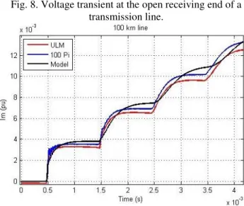
In this section, the frequency-dependent Bergeron line model output is compared with the well-established Universal Line Model – ULM and a frequency dependent
cascade of π circuits with 100 sections for a 100km length transmission line.
Initially, two extreme cases are simulated to highlight voltage and current transients in transmission lines. The first case consists of a switching operation at the sending terminal of the line with the receiving terminal in open-circuit. The second case is the same transmission line under the same conditions with the receiving end in short-circuit (approximately 3.7 Ω) [7].
Results obtained for both cases are shown in Fig. 8 and Fig. 9.
Fig. 8. Voltage transient at the open receiving end of a transmission line.
Fig. 9. Current transient at the receiving end of a transmission line under short-circuit conditions.
Although both models, cascade of π circuits and frequency-dependent Bergeron model, are time-domain based models and produce a similar output, it can be noted that frequency-dependent Bergeron model is significantly
faster than the cascade of π circuits. Processing times for both models are shown in Table 1.
TABLE I. PROCESSING TIMES OF TIME-DOMAIN BASED MODELS
cascade of π
circuits
frequency-dependent Bergeron model Open circuit
simulation
19.64 [s] 3.28 [s]
Short circuit simulation
19.75 [s] 3.26 [s]
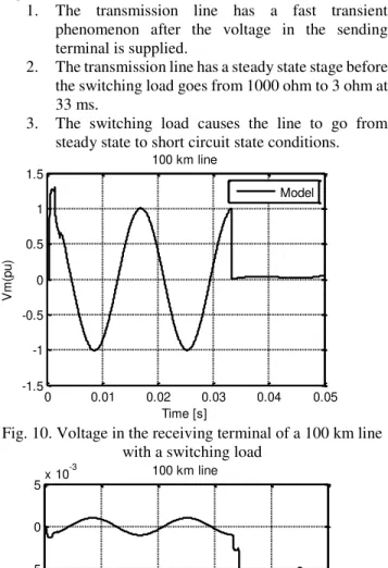
ohm at 33 ms, when the 1000 ohm load is already in steady state conditions. Voltage and current obtained on the receiving terminal of the line are shown in Fig. 10 and Fig. 11 respectively.
It can be noted that the transmission line goes through 3 stages:
1. The transmission line has a fast transient phenomenon after the voltage in the sending terminal is supplied.
2. The transmission line has a steady state stage before the switching load goes from 1000 ohm to 3 ohm at 33 ms.
3. The switching load causes the line to go from steady state to short circuit state conditions.
Fig. 10. Voltage in the receiving terminal of a 100 km line with a switching load
Fig. 11. Current on the receiving terminal of a 100 km line with a switching load
V. CONCLUSIONS
The inclusion of the frequency effect in the Bergeron line model using fitting techniques can be used to simulate low to medium frequency phenomena. The model was compared with the the well established Universal Line Model – ULM, giving satisfactory results. In addition, the model was compared to other time domain model that includes the frequency effect among its parameters. The main attributes of the frequency-dependent Bergeron model can be resumed as follow:
Less computational effort
Solution found directly in the time domain, so power electronics and nonlinear devices can be used in simulations
Less oscillations due to time discretization compared to other time-domain models
Similar results with other well-established models In short, the model shows good accuracy, and good computational performance while simulating low to medium frequency phenomena. In addition, it can be used with non linear elements directly represented in the time domain.
VI. BIBLIOGRAPHY
[1] F. U. P. GOMES, "The numerical Laplace transform: an accurate technique for analyzing electromagentic transients on power system devices," Int. Journal of Elect. Power & Energy Systems, vol. 31, no. 2-3, pp. 116-123, 2009.
[2] M. S. MAMIS and M. MERAL, "State-space modeling and analysis of fault arcs," Electr. Power Syst., pp. 46-51, 2005.
[3] A. Ametani, N. Nagaoka, T. Noda and T. Matsuura, "A simple and efficient method for including frequency-dependent effects in transmission line transient analysis," Int. Journal of Elect. Power & Energy Systems, vol. 19, no. 4, pp. 225-261, 1997. [4] F. J. Branin, "Computer methods of network
analysis," Proceedings of the IEEE, vol. 55, no. 11, pp. 1787-1801, 1967.
[5] H. W. Dommel, Electromagnetic Transient Program Reference Manual (EMTP theory book), Vancouver: Dept. Electrical Engineering, 1989.
[6] J. Snelson, "Propagation of travelling waves on transmission lines: frequency dependent parameters," Power Apparatus and Systems, IEEE Transactions on, Vols. PAS-91, no. 1, pp. 85 - 91, 1972. [7] E. Costa, S. Kurokawa, J. Pissolato and A. Prado,
"Efficient procedure to evaluate electromagnetic transients on three-phase transmission lines," IET Generation Transmission & Distribution, vol. 4, no. 9, pp. 1069-1081, 2010.
[8] B. Gustavsen and A. Semlyen, "Combined phase and modal domain calculation of transmission line transients based on vector fitting," Power Delivery, IEEE, vol. 13, no. 2, pp. 596-604, 1998.
[9] P. Caballero, E. Costa and S. Kurokawa, "Fitting the frequency-dependent parameters in the the Bergeron line model," ELSEVIER, vol. 117, pp. 14-20, 2014. [10] C. F. Gerald and P. O. Wheatley, Applied Numerical
Analysis, Addison-Wesley, 1994.
0 0.01 0.02 0.03 0.04 0.05
-1.5 -1 -0.5 0 0.5 1 1.5
100 km line
Time [s]
V
m
(p
u
)
Model
0 0.01 0.02 0.03 0.04 0.05
-20 -15 -10 -5 0 5x 10
-3 100 km line
Time [s]
Im
(p
u
)