River inflow and retention time affecting spatial heterogeneity of chlorophyll and water–air CO<sub>2</sub> fluxes in a tropical hydropower reservoir

(1)

BGD

11, 8531–8568, 2014

Spatial heterogeneity of Chl and CO2 fluxes

F. S. Pacheco et al.

Title Page

Abstract Introduction

Conclusions References

Tables Figures

◭ ◮

Back Close

Full Screen / Esc

Printer-friendly Version

Interactive Discussion

Discussion

P

a

per

|

Discus

sion

P

a

per

|

Discussion

P

a

per

|

Discussion

P

a

per

|

Biogeosciences Discuss., 11, 8531–8568, 2014 www.biogeosciences-discuss.net/11/8531/2014/ doi:10.5194/bgd-11-8531-2014

This discussion paper is/has been under review for the journal Biogeosciences (BG). Please refer to the corresponding final paper in BG if available.

River inflow and retention time a

_ff

ecting

spatial heterogeneity of chlorophyll and

water–air CO

₂

fluxes in a tropical

hydropower reservoir

F. S. Pacheco1, M. C. S. Soares2, A. T. Assireu3, M. P. Curtarelli4, F. Roland2, G. Abril5, J. L. Stech4, P. C. Alvalá1, and J. P. Ometto1

1

Earth System Science Center, National Institute for Space Research, São José dos Campos, 12227-010, São Paulo, Brazil

2

Laboratory of Aquatic Ecology, Federal University of Juiz de Fora, Juiz de Fora, 36036-900, Minas Gerais, Brazil

3

Institute of Natural Resources, Federal University of Itajubá, Itajubá, 37500-903, Minas Gerais, Brazil

4

Remote Sense Division, National Institute for Space Research, São José dos Campos, 12227-010, São Paulo, Brazil

5

(2)

BGD

11, 8531–8568, 2014

Title Page

Tables Figures

◭ ◮

Back Close

Full Screen / Esc

Discussion

P

a

per

|

Discus

sion

P

a

per

|

Discussion

P

a

per

|

Discussion

P

a

per

|

Received: 15 April 2014 – Accepted: 6 May 2014 – Published: 11 June 2014

Correspondence to: F. S. Pacheco (felipe.pacheco@inpe.br)

(3)

BGD

11, 8531–8568, 2014

Title Page

Tables Figures

◭ ◮

Back Close

Full Screen / Esc

Discussion

P

a

per

|

Discus

sion

P

a

per

|

Discussion

P

a

per

|

Discussion

P

a

per

|

Abstract

Much research has been devoted to understanding the complexity of biogeochemical and physical processes responsible for the greenhouse gas (GHG) emissions from hy-dropower reservoirs. Spatial complexity and heterogeneity of GHG emission may be observed in these systems because it is dependent on flooded biomass, river inflow, 5

primary production and dam operation. In this study, we investigate the relationships

between water–air CO₂fluxes and phytoplanktonic biomass in Funil Reservoir, an old

and stratified tropical reservoir, where intense phytoplankton blooms and low partial

pressure of CO2 (pCO2) are observed. Our results showed that Funil Reservoir

sea-sonal and spatial variability of chlorophyll concentration (Chl) and pCO₂ is more

re-10

lated to changes in river inflow over the year than environmental factor such as air temperature and solar radiation. Field data and hydrodynamic simulations reveal that the river inflow contributes to increased heterogeneity in dry season due to the vari-ation of reservoir retention time and river temperature. Contradictory conclusion can be drawn if temporal data collected only near the dam is considered instead of spatial 15

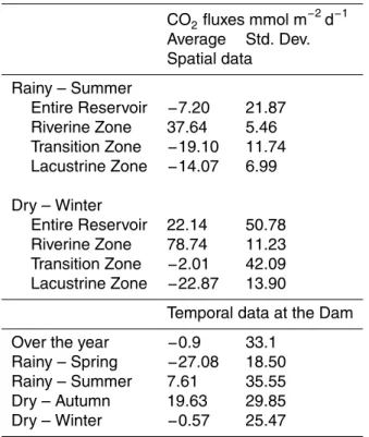
data to represent CO₂fluxes in whole reservoir. The average CO₂fluxes was−17.6 and

22.1 mmol m−2

d−2

considering data collected near the dam and spatial data, respec-tively, in periods of low retention time. In this case, the lack of spatial information can change completely the role of Funil Reservoir regarding GHG emissions. Our results support the idea that Funil Reservoir is a dynamic system where the hydrodynamics 20

represented by changes in river inflow and retention time is potentially more important

force driving both Chl andpCO2spatial variability than in-system ecological factors.

1 Introduction

Over the last two decades, hydropower reservoirs have been identified as potentially important sources of greenhouse gas (GHG) emissions (St Louis et al., 2000; Rosa 25

(4)

flood-BGD

11, 8531–8568, 2014

Title Page

Tables Figures

◭ ◮

Back Close

Full Screen / Esc

Discussion

P

a

per

|

Discus

sion

P

a

per

|

Discussion

P

a

per

|

Discussion

P

a

per

|

ing of large amounts of biomass, including primary forest, result to intense GHG emis-sion (Abril et al., 2005; Fearnside and Pueyo, 2012). However, emisemis-sions are larger in tropical Amazonian (Abril et al., 2013) than in tropical Cerrado reservoirs (Ometto et al., 2011) and in younger than in older reservoirs (Barros et al., 2011). Large hydroelectric reservoirs, especially those created by impounding rivers, are morphometrically com-5

plex and spatially heterogeneous (Roland et al., 2010; Teodoru et al., 2011; Zhao et al.,

2013). Diff_{erent regions in terms of CO}

2 may be observed in these systems because

it is dependent on flooded biomass, river input of organic matter, primary production and dam operation regime. Furthermore, both heterotrophic and autotrophic activity

influences CO₂concentration along reservoirs and the role of these activities has been

10

reported in subtropical (Di Siervi et al., 1995), tropical (Roland et al., 2010; Kemenes et al., 2011) and temperate areas (Richardot et al., 2000; Lauster et al., 2006; Finlay et al., 2009; Halbedel and Koschorreck, 2013).

As the sedimentation and light availability increase along the reservoir, biomass of primary producers may increase. The phytoplankton is distributed in patches along 15

the reservoir due to diff_{erences in habitat conditions linked to nutrient distribution, light}

availability and stratification (Serra et al., 2007). Also, hydrodynamics factors as re-tention time and river inflow showed to influence the phytoplankton communities and growth (Vidal et al., 2012; Soares et al., 2008). Intense phytoplankton primary pro-duction has been identified as the main regulator of carbon (C) budget in temperate 20

eutrophic lakes (Finlay et al., 2010; Pacheco et al., 2014), however the impact on trop-ical hydropower reservoir is still unclear.

River inflows may aff_{ect biogeochemical patterns in river valley reservoirs (Kennedy,}

1999). Diff_{erence on density of the incoming stream and lake water, stream and lake}

hydraulics, strength of stratification and mixing are features that control how the river 25

water will flow when it reaches the reservoir (Fischer and Smith, 1983; Fischer et al.,

1979). As result of density diff_{erences between river and lake water, the river enters in}

(5)

BGD

11, 8531–8568, 2014

Title Page

Tables Figures

◭ ◮

Back Close

Full Screen / Esc

Discussion

P

a

per

|

Discus

sion

P

a

per

|

Discussion

P

a

per

|

Discussion

P

a

per

|

and the dynamic of river inflow can determine the spatial heterogeneity in

phytoplank-ton distribution (Vidal et al., 2012). Consequently, river inflow may aff_{ect primary}

pro-duction along river/dam axis in hydropower reservoirs strongly influenced by river. In this study, we investigate the relationships between phytoplanktonic biomass and

water–air CO2fluxes in an old and stratified tropical reservoir (Funil, state of RJ, Brazil),

5

where intense phytoplankton blooms and low pCO2 are observed in the water. We

combine fieldwork and modeling to analyze the respective impact of meteorological and hydrological factors on the spatial and temporal dynamics of phytoplankton and

the intensity of CO2 fluxes. We show the effect of the river inflow in the heterogeneity

ofpCO₂and Chl in Funil reservoir. We also compare temporal data ofpCO₂collected

10

near the dam with a high dense spatial data. Our hypothesis were that (1) seasonal and

spatial variability ofpCO2and Chl in Funil Reservoir is more related to river inflow and

retention time than external environmental factor such as air temperature and solar

radiation and, (2) very diff_{erent conclusion can be drawn regarding carbon cycle in}

reservoir if spatial heterogeneity is not adequately considered. 15

2 Materials and methods

2.1 Study site

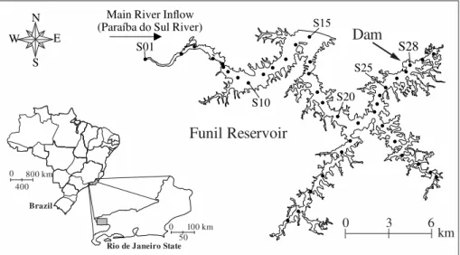
Funil Reservoir is an old impoundment constructed at the end of the 1960s and is located on Paraíba do Sul River, in a southern city (Resende) of the Rio de Janeiro

State, Brazil (22◦30′S, 44◦45′W, Fig. 1). It is 440 m a.s.l., with wet-warm summers and

20

dry-cold winters (Cwa, Köppen system). The main purpose of Funil Reservoir is energy production, but the reservoir is also used for irrigation and recreation. It has a surface

area of 40 km2, mean and maximum depth of 22 and 74 m, respectively, and total

volume of 890×106m3. The maximum and minimum reservoir water level occurs in the

(6)

BGD

11, 8531–8568, 2014

Title Page

Tables Figures

◭ ◮

Back Close

Full Screen / Esc

Discussion

P

a

per

|

Discus

sion

P

a

per

|

Discussion

P

a

per

|

Discussion

P

a

per

|

to September 2012, the diff_{erence between minimum and maximum water level was}

15.6 m.

Funil Reservoir has a catchment area of 12 800 km2 that has a high demographic

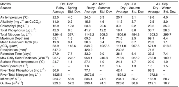
density. The river inflow is not restrictedly linked to the rainfall in the watershed because it also depends on the water supply-demand and operation of dams constructed up-5

stream. There are around 2 million people living inside the catchment area and 39 cities depending on the Paraíba do Sul River for water supply. These cities comprises 2 % of Brazil’s gross domestic product (GDP) (IBGE, 2010). In this area, 46 % of sewage is untreated (AGEVAP, 2011) and the Paraiba do Sul River receives a large portion of the sewage from one of the main Brazilian industrial areas crossing part of the São 10

Paulo State. Consequently, the river has a large influence on reservoir’s water qual-ity that has experienced tragic eutrophication in recent decades, resulting in frequent and intense cyanobacterial blooms (Klapper, 1998; Branco et al., 2002; Rocha et al., 2002). In general, Funil Reservoir is a turbid, eutrophic system, with high phytoplankton (cyanobacteria) biomass (Soares et al., 2012; Rangel et al., 2012).

15

2.2 Field sampling

Spatial data– the water samples for Chl and pCO₂ were taken between 09:00 LT and 12:00 LT on 1 March 2012 (end of rainy season, high water lever) and 20 Septem-ber 2012 (end of dry season, low water level). Samples were taken at the surface (0.3 m) at 42 stations in Funil Reservoir (28 located along the main body of the reser-20

voir, Fig. 1) in the same day to limit the eff_{ect of diurnal variation on the results.}

We measured the Chl using a compact version of PHYTO-PAM (Heinz Walz GmbH,

PHYTO-ED, Eff_{elrich, Germany). Functionally the PHYTO-ED displays the same}

fea-tures as the standard but has distinct advantages for fieldwork. In the PHYTO-PAM Phytoplankton Analyzer µsec measuring light pulses are generated by an array of light-25

emitting diodes (LED) featuring 4 diff_{erent colors: blue (470 nm), green (520 nm), light}

red (645 nm) and dark red (665 nm). The diff_{erently colored measuring light pulses are}

(7)

BGD

11, 8531–8568, 2014

Title Page

Tables Figures

◭ ◮

Back Close

Full Screen / Esc

Discussion

P

a

per

|

Discus

sion

P

a

per

|

Discussion

P

a

per

|

Discussion

P

a

per

|

Chl fluorescence excited at the 4 diff_{erent wavelengths is obtained. Following proper}

calibration, this feature allows to diff_{erentiate between the contributions of the main}

types of phytoplankton (green, blue, brown algae) with diff_{erent pigment systems. In}

addition, Chl content of the various types can be estimated.

The pCO2 data were determine using water–air equilibration method. In a

marble-5

type equilibrator (Abril et al., 2014, 2006), water pumped directly from the lake flows from the top to the bottom (0.8 liters per min), while a constant volume of air (0.4 liters per min) flows from the bottom to the top. The large gas exchange surface area

pro-moted by the contact with the marbles accelerates the pCO2 water–air equilibrium.

The air pump conduct the air from the top of the equilibrator through a drying tube con-10

taining a desiccant (Drierite), then to an infrared gas analyzer (IRGA, LI-840, LICOR, Lincoln, Nebraska, USA), and then back to the bottom of the equilibrator (closed air cir-cuit, Abril et al., 2006). For each station, the lake water and air were pumped through

this system for two minutes before thepCO₂ from the IRGA stabilized to a constant

value. 15

Color maps were created to represent spatial distribution of Chl andpCO2(Fig. 2).

We used variogram analysis to describe spatial correlation among samples and to spatially interpolate using Kriging methods (Bailey and Gatrell, 1995). The empirical

variograms were fitted to diff_{erent mathematical models using Akaike’s information}

cri-terion (AIC, Akaike, 1974) to evaluate the best fit. The best model variogram were 20

used for interpolation by ordinary kriging. The root mean-square error (RMSE),

calcu-lated comparing observed and calcucalcu-lated values, was 90 µatm and 15 µg L−1forpCO2

and Chl, respectively. We used the software Spring (Câmara et al., 1996) version 5.1.8

to conduct the spatial analysis and to produce the in situpCO2and Chl maps.

Time series data– wind speed and direction, solar radiation, pH, dissolved oxygen 25

(8)

BGD

11, 8531–8568, 2014

Title Page

Tables Figures

◭ ◮

Back Close

Full Screen / Esc

Discussion

P

a

per

|

Discus

sion

P

a

per

|

Discussion

P

a

per

|

Discussion

P

a

per

|

monitoring of hydrological systems (Alcantara et al., 2013; Stevenson et al., 1993). The SIMA consists of an independent system formed by an anchored buoy containing data storage systems, sensors (air temperature, wind direction and intensity, pressure, incoming and reflected radiation and a thermistor chain), a solar panel, a battery and a transmission antenna. A sonde (YSI model 6600, Yellow Spring, Ohio, USA) was 5

attached to the SIMA buoy to collect hourly surface data on temperature, conductiv-ity, pH, and oxygen. This sonde was calibrated every 15 days according to the YSI Environmental Operations Manual (http://www.ysi.com/ysi/support).

We calculated thepCO2in the surface water over one year near the dam from

mea-sured pH and alkalinity. The calculations include dependence on temperature for disso-10

ciation constants of carbonic acid (Millero et al., 2002) and solubility of CO₂. We used

pH and temperature collected by SIMA between 25 October 2011 and 25 October 2012 and monthly data of alkalinity determined by the titration method (APHA, 2005) at sta-tion S28 (Fig. 1). Samples for total phosphorous (TP) and nitrogen (TN) were taken monthly. For TP, the samples was oxidized by persulfate and then analyzed as soluble 15

reactive phosphorus. TN was determined as the sum of organic fraction measured by Kjedahl method and the dissolved inorganic nutrients. Laboratory analysis for TP and NP was performed according to standard spectrophotometric techniques (Wetzel and Likens, 2010).

2.3 CO2flux calculation

20

The air-water flux of CO₂(mmol m−2

d−1

) was calculated according to Eq. (1).

F(CO₂)=_kα∆_p_CO

2 (1)

Wherek is the gas transfer velocity of CO2(in cm h−

1

),α is the solubility coeffi_{cient of}

CO2(in mol kg−

1

atm−1) as a function of water temperature (Weiss, 1974), and∆_p_CO₂

25

is the air-water gradient ofpCO₂ (in µatm). The atmospheric pCO₂ measured in the

(9)

BGD

11, 8531–8568, 2014

Title Page

Tables Figures

◭ ◮

Back Close

Full Screen / Esc

Discussion

P

a

per

|

Discus

sion

P

a

per

|

Discussion

P

a

per

|

Discussion

P

a

per

|

calculation. The gas transfer velocity k was calculated from the gas transfer velocity

normalized to a Schmidt number of 600 that corresponds to CO2at 20◦C (Eq. 2) (Jahne

et al., 1987). Positive values of CO2 fluxes denotes net gas flux from the lake to the

atmosphere.

k=k₆₀₀

600 Sc

−0,5

(2) 5

Wherek₆₀₀is the normalized gas transfer velocity calculated according to the following

equation (Cole and Caraco, 1998),Scis the Schmidt number of a given gas at a given

temperature (Wanninkhof, 1992).

k₆₀₀=_2.07+_0.21_U1.7

10 (3)

10

WhereU₁₀is wind speed at 10 m height. The wind speed was obtained from the SIMA

da at 3 m height and was calculated for 10 m height (Smith, 1985).

In riverine zone, we considered thek₆₀₀as a function of wind and water current. The

contribution of the water current to the gas transfer velocity was estimated using the 15

water current (cm s−1), depth (m) and the equations in Borges et al. (2004).

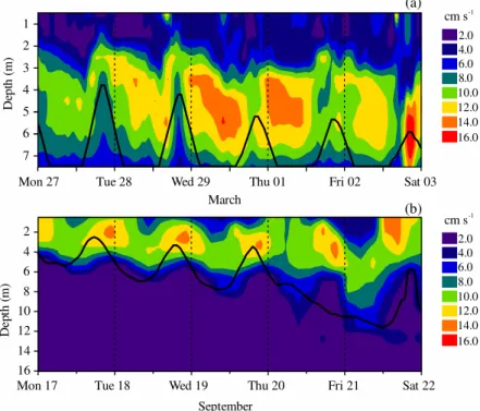
2.4 Temperature profile

Temperature profiles were collected using thermistor chain deployed at station S09 in rainy season and station S14 in dry season to determine the thermal structure at transi-tion zone. Eleven thermistors (Hobo, U22 Water Temp Pro v2, Bourne, Massachusetts, 20

USA) were placed every 0.5 m up to 4 m and every 1 m from 5 to 7 m. We also deployed a thermistor chain at riverine zone at station S05 with thermistors placed every 2 m. The thermistors were programed to record temperature every 10 min. In the rainy season, the thermistor chain was deployed on 29 February 2012 at 18:30 LT and recovered af-ter 40 h. In the dry season, the thermistor chain was deployed on 20 September 2012 25

(10)

BGD

11, 8531–8568, 2014

Title Page

Tables Figures

◭ ◮

Back Close

Full Screen / Esc

Discussion

P

a

per

|

Discus

sion

P

a

per

|

Discussion

P

a

per

|

Discussion

P

a

per

|

In our analysis, temperature is considered as the factor controlling water density. The use of temperature is justified by the low conductivity and turbidity in the river. The values of turbidity measured in the field of 29 and 11 NTU in rainy and dry seasons,

respectively, would have eff_{ected density}_<_{5 % relative to that of temperature (Gippel,}

1989). 5

2.5 Numerical Model description and setup

Numerical simulations of lake hydrodynamics were conducted with the Estuary and Lake Computer Model (ELCOM, Hodges et al., 2000), which solves the 3-D hydro-static, Boussinesq, Reynolds-averaged Navier–Stokes and scalar transport equations, separating mixing of scalars and momentum from advection. The hydrodynamic al-10

gorithms that are implemented in ELCOM use an Euler–Lagrange approach for the advection of momentum adapted from the work of Casulli and Cheng, 1992, whereas the advection of scalars (i.e., tracers, conductivity and temperature) is based on the UL-TIMATE QUICKEST method proposed by Leonard, 1991). The thermodynamics model considers the penetrative (i.e., shortwave radiation) and non-penetrative components 15

(i.e., longwave radiation, sensible and latent heat fluxes) (Hodges et al., 2000). The vertical mixing model uses the transport equations of turbulent kinetic energy (TKE) to compute the energy available from wind stirring and shear production for the mix-ing process (Spigel and Imberger, 1980). A complete description of the formulae and numerical methods used in ELCOM was given by Hodges et al. (2000).

20

Simulations of hydrodynamics of Funil reservoir were conducted with realistic forcing condition (e.g. inflow, outflow, atmospheric temperature, radiation). These simulations were aimed in order to test the hypothesis regarding the river inflows at transition zone in rainy and dry seasons in Funil reservoir. Simulations started 4 days before the date of the considered data. This is necessary to let the model equilibrate beyond the initial 25

physical conditions. The numerical domain was discretized in a uniform horizontal grid

containing 100 m×100 m cells based on a depth sample. The depth data were

(11)

BGD

11, 8531–8568, 2014

Title Page

Tables Figures

◭ ◮

Back Close

Full Screen / Esc

Discussion

P

a

per

|

Discus

sion

P

a

per

|

Discussion

P

a

per

|

Discussion

P

a

per

|

1 m thickness, resulting in 72 vertical layers. The water albedo was set to 0.03 (Slater,

1980), and the bottom drag coeffi_{cient was set to 0.001 (Wüest and Lorke, 2003). The}

attenuation coeffi_{cient for PAR was set to 0.6 m}−1_{based on Secchi disc measurements.}

A value of 5.25 m2s−1, based on a previous study conducted in another tropical

reser-voir (Pacheco et al., 2011), was chosen for the horizontal diff_{usivity for temperature and}

5

for the horizontal momentum.

Because of the presence of persistent unstable atmospheric conditions over tropi-cal reservoirs (Verburg and Antenucci, 2010), the atmospheric stability sub-model was activated during the simulation; this procedure is appropriate in the cases in which the meteorological sensors are located within the internal atmospheric boundary layer 10

(ABL) over the surface of the lake and data are collected at sub-daily intervals

(Im-berger and Patterson, 1990). In this manner, the heat and momentum transfer coeffi

-cients were adjusted at each model time step based on the stability of the ABL. The Coriolis sub-model was also activated during the simulation.

We defined two sets of boundary cells to force the inflow (Paraíba do Sul River) 15

and outflow: (the water intake at the dam). The meteorological driving forces over the free surface of the reservoir were considered uniform. The model was forced using hourly meteorological data acquired by SIMA, the daily inflow and outflow provided by Eletrobrás-Furnas and the cloud cover and river temperatures extracted from thermis-tor chain data and complemented with MODIS data. Two periods were simulated: one 20

to represent rainy season (25 February 2012 to 4 March 2012) and one to represent dry season (15 to 23 September 2012).

3 Results

3.1 Spatial variability

Based on spatial data of Chl and pCO₂, a typical zonation pattern usually found in

25

(12)

BGD

11, 8531–8568, 2014

Title Page

Tables Figures

◭ ◮

Back Close

Full Screen / Esc

Discussion

P

a

per

|

Discus

sion

P

a

per

|

Discussion

P

a

per

|

Discussion

P

a

per

|

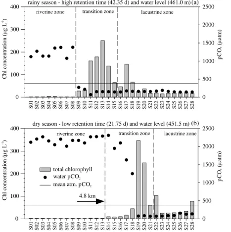
(Fig. 2). Although the boundaries are influenced by many factors and are not easily determined, these regions have distinct physical, chemical and biological features. The riverine zone (RZ) has a high input of nutrients coming from terrestrial systems and hu-man activities, but the primary production is limited by high turbidity and turbulence. As the sedimentation and light availability increase along the reservoir, biomass of primary 5

producers increases in the transition zone (TZ). The lacustrine zone (LZ) is character-ized by nutrient limitation and reduced phytoplankton biomass (Thornton, 1990). In this study, we considered the Chl to separate the reservoir in three zones. Riverine zone

is characterized by low Chl (<5 µg L−1). Transition zone begins where the Chl starts

to increase and ends when Chl decrease to levels closely to Chl in Lacustrine zone. 10

Finally, Lacustrine zone is characterized by intermediate Chl.

Funil reservoir showed to be spatially heterogeneous with seasonal diff_{erences in}

Chl andpCO2(Fig. 2). The spatial data showed high spatial variation only in the main

body of the reservoir, while the southern part was undersaturated in CO₂in rainy and

dry seasons (Fig. 2a and b). Spatially average ofpCO2for rainy and dry season were

15

259±221 and 881±900 µatm, respectively. ThepCO2 varied from 140 to 1376 µatm

in rainy season and from 43 to 2290 µatm in dry season. Higher values ofpCO₂in the

riverine zone of the reservoir and a drastically decrease in the transition zone were ob-served in both sample periods (Fig. 3a and b). In the lacustrine zone, undersaturation

on CO₂was prevalent at all sample sites in rainy and dry season. Considering all

sam-20

ple sites, there was significant diff_{erences between rainy and dry seasons (}_t=_1.99,

p <0.05) and higher values ofpCO2 during dry season in Funil reservoir were

previ-ously reported (Roland et al., 2010). Chl was higher in the transition zone compared

with others compartments (t=_2.01, _{p <}_{0.05, Fig. 3a and b). Further, average}

con-centration in transition zone was 2.5 times higher than the reservoir average (129.2 25

and 52.0 µg L−1_{, respectively). Unlike}_p_CO

2, Chl data showed no significant difference

between rainy and dry season considering all spatial data (t=_1.99,_{p >}_0.05).

The calculated CO2fluxes from spatial data varied from−35.8 to 44.2 mmol m−

2

d−1

(13)

BGD

11, 8531–8568, 2014

Title Page

Tables Figures

◭ ◮

Back Close

Full Screen / Esc

Discussion

P

a

per

|

Discus

sion

P

a

per

|

Discussion

P

a

per

|

Discussion

P

a

per

|

dry seasons, the maximum emission was observed in riverine zone and the minimum

in the transition zone. The spatial average was−7.2 and 22.1 mmol m−2d−1in the rainy

and dry season, respectively (Table 1).

3.2 Temporal variability

ThepCO2 calculated by multi-parameter sonde data (temperature and pH) and

alka-5

linity showed a large seasonal variability over the year at the station near the dam

(Table 2). ThepCO2 varied from 35 to 4058 µatm with average of 624±829 µatm and

median of 165 µatm. ThepCO2supersaturation was prevalent between April and June,

while pCO₂ undersaturation was prevalent in all other periods (Fig. 4a). Lowest

me-dian ofpCO2 was observed between October and December (43 µatm). Considering

10

all temporal data over the year, 59.8 % of the data were below atmospheric equilibrium and 1.1 % were within 5 % of atmospheric equilibrium.

In Funil Reservoir, the seasonalpCO₂variation over the year at the station near the

dam agreed with variation of retention time (Fig. 4). The yearly average of the reservoir retention time was 32.6 days over the considered year. Lower retention time occurs 15

between October and December when the water level is low and the reservoir is ready to stock water coming from the watershed and rain during the rainy season (October to March).

The CO₂ flux over the year at the station near the dam varied from −119.8 to

234.5 mmol m−2d−1. The average of flux was−0.9±33.1 mmol m−2d−1and median of

20

−6.2 mmol m−2d−1. We observed substantial uptake of CO2between October and

De-cember (rainy-spring) (Table 1). Uptake of CO₂from the atmosphere was also prevalent

between July and September (dry-winter). From January to July, the lake lost

substan-tial CO2via degassing (Table 1). Summary of all other data collected over the studied

(14)

BGD

11, 8531–8568, 2014

Title Page

Tables Figures

◭ ◮

Back Close

Full Screen / Esc

Discussion

P

a

per

|

Discus

sion

P

a

per

|

Discussion

P

a

per

|

Discussion

P

a

per

|

3.3 Thermal structure of transition zone and river

During the rainy season, thermal stratification occurred in the transition zone only

dur-ing the daytime around 16:30 LT, when a maximum of 33.1◦C was observed at the

sur-face for a minimum of 27.8◦_{C at the bottom (Fig. 5a); to the contrary, temperature was}

vertically homogeneous at nighttime. The daily range of temperature oscillation during 5

rainy season at surface was up to 5◦C. In the dry season, water temperature were

lower compared to the rainy season at transition zone. Stratification occurred around

14:00 LT in dry season, when we observed a maximum of 25.7◦C and a minimum of

23.1◦C at the bottom. The daily range of temperature oscillation was up to 3◦C at

sur-face and stratus layers with diff_{erent temperatures were observed every 2.5 m (Fig. 5b).}

10

The river temperature varied from 27.7 to 28.7◦C and 23.6 to 24.1◦C in rainy and dry

season, respectively (Table 3). The average temperature diff_{erence between river and}

reservoir surface water was 2.1 and 0.3◦_{C in rainy and dry season, respectively.}

3.4 Simulations

We first compared the simulated and real temperature at station S09 and S14 for rainy 15

and dry season, respectively. The RMSE, calculated by comparing data every 20 min

were 1.4◦_{C for rainy season and 1.1}◦_{C for dry season. These results obtained for both}

seasons are comparable with previous modelling exercises found in literature (Jin et al., 2000; Vidal et al., 2012). We also analyzed the ability of the model to reproduce the in-flow using data from drifters released in the river and transition zone of the reservoir on 20

1 March and 20 September (data not shown). Although the vertical thermal structures observed in dry season (Fig. 5b) were not well represented, the model reproduced the behavior of the inflow as underflow in rainy season (Fig. 6a) and interflow and overflow in dry season (Fig. 6b) as anticipated by the schematic representation (Fig. 5c and d). The river flowed mainly at 6 m depth near the bottom of Funil reservoir after the river 25

(15)

BGD

11, 8531–8568, 2014

Title Page

Tables Figures

◭ ◮

Back Close

Full Screen / Esc

Discussion

P

a

per

|

Discus

sion

P

a

per

|

Discussion

P

a

per

|

Discussion

P

a

per

|

The daily oscillation of the neutral buoyance observed occurs because of the variation of reservoir surface and river temperatures (Vidal et al., 2012; Curtarelli et al., 2013). The level of neutral buoyancy, where the densities of the flowing current and the ambient fluid are equal, represents the depth where the river water spreads laterally in the reservoir. In rainy season, the river flowed as underflow (Fig. 6a), how-5

ever, when the river reached its maximum temperature around 21:00 LT (Table 3) the

temperature diff_{erence between river and surface water decreased, the level of river}

neutral buoyance moved upward and the maximum flow was observed between 4 and 6 m (Fig. 6a). In the dry season, the river flowed as overflow, but it plunged down to 4 to 6 m depth when the high surface temperature during the day coincided with the period 10

of lowest river temperature (Table 3) and neutral buoyance moved downward (Fig. 6b). The change in patterns observed in the river flow between 20 and 21 September oc-curred due to a decrease of the river temperature during a rainfall that ococ-curred around 16:00 LT on 20 September 2012 (Fig. 6b).

4 Discussion

15

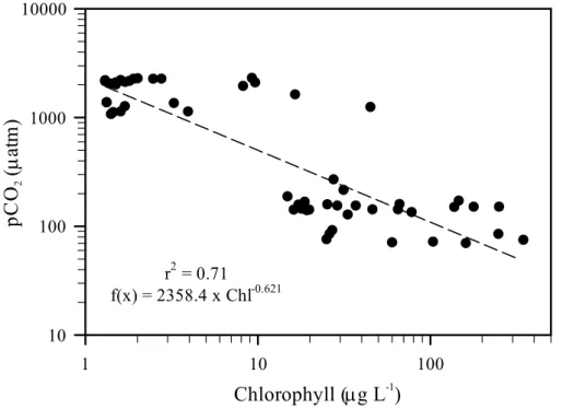
4.1 pCO₂driven by Phytoplankton

Primary production associated to the high Chl showed to be the main regulator of

CO₂concentration at the surface of the Funil Reservoir (Fig. 7). Spatially, pCO₂were

negatively correlated to the Chl (r2=_{0.71). In old hydropower reservoir where C source}

from the flooded soil after impounding has become negligible, primary production may 20

become a significant term in the C budget. Intense primary production fuelled by high

levels of nutrients reduces CO₂concentrations to levels below atmospheric equilibrium

in transition zone and lacustrine zone (Fig. 3). To the contrary, high values of pCO2

in riverine zone may be associated with suspended solids and turbulence and vertical mixing that inhibit primary production.

(16)

BGD

11, 8531–8568, 2014

Title Page

Tables Figures

◭ ◮

Back Close

Full Screen / Esc

Discussion

P

a

per

|

Discus

sion

P

a

per

|

Discussion

P

a

per

|

Discussion

P

a

per

|

LowpCO₂ levels observed at the station near the dam over the year is associated

with (1) high primary production due to higher temperature and solar radiation that pro-mote water column stability and stratification, and (2) constant high nutrient availability. Since nutrient availability in Funil Reservoir is high during the entire year (Table 2), nutrients are never limited in the lacustrine zone and other factors that controls stability 5

and stratification, such as temperature, wind and changes in mixing depth related to the seasonal variation are the main inhibitors of algal growth near the dam especially between April and June.

Due to phytoplankton productivity, we found net uptake of CO2over the year at the

station near the dam, especially between October and December (Table 1). The fate 10

of carbon fixed by the phytoplankton in Funil Reservoir is still unclear. The higher flux

of methane (CH4) from sediment to water found in Funil Reservoir compared to other

tropical reservoir (Ometto et al., 2013) suggests that a substantial fraction of the fixed

carbon reaches the sediment and is further mineralized in CH₄. However, in lacustrine

zone, the higher depth and high temperature may promote mineralization of part of 15

carbon fixed by phytoplankton in the water column before it reaches the sediment. Outflow export the same amount of carbon that comes from the watershed (Ometto et al., 2013), so the water that flows through the turbine is not responsible to export the excess of carbon invaded from the atmosphere. Although there is no data to support this statement, as reported in natural eutrophic lakes (Downing et al., 2008), burial 20

of organic carbon composed by phytoplankton and methanogenesis seems to be two important carbon pathways for the carbon fixed by the phytoplankton in Funil Reservoir.

4.2 Physical feature and spatial distribution

The retention time of Funil reservoir is strongly driven by the operation of the dam. The volume of water that flows through the turbine depends on the energy demands and 25

(17)

BGD

11, 8531–8568, 2014

Title Page

Tables Figures

◭ ◮

Back Close

Full Screen / Esc

Discussion

P

a

per

|

Discus

sion

P

a

per

|

Discussion

P

a

per

|

Discussion

P

a

per

|

is full to ensure enough water to produce energy during entire dry season. Therefore, many ecological processes in natural lakes that are related with external factor (e.g. solar radiation, precipitation and temperature) may be regulated by dam operation in hydropower reservoir.

The position of transition zone of the reservoir moves as result of the seasonally 5

(Fig. 3). In the end of the rainy season, the retention time and water level was high, and the influence of the river in the surface water of the reservoir was restrict to a small

area (Fig. 2a and c). Diff_{erently, when the water level and retention time was low, the}

transition zone moved toward the dam and the river inflow influenced the surface Chl

andpCO₂in more than 40 % of the total reservoir surface area (Fig. 2b and d). A

reser-10

voir can become a fluvial-dominated system when retention time is short or lacustrine

when retention time is long (Straš_{kraba, 1990).}

Size of the river-influenced area in the reservoir surface water also depends on

wa-ter density. Diff_{erences on river and reservoir temperature, total dissolved solids, and}

suspended solids can cause density gradient in the water column. Depending on the 15

water density diff_{erences between the inflow and reservoir, the river can flow into the}

downstream area as overflow, underflow, or interflow (Martin and McCutcheon, 1998).

During the rainy season in Funil reservoir, due to the high diff_{erence between river and}

reservoir surface temperature (∼4◦C), the river water progressively sinks down

(un-derflow), and contributes to the thermal stability of the water column (Fig. 5a, Assireu 20

et al., 2011). The denser river water flows under a lighter reservoir water and waves and billows develops along the interface due to shear velocity. This behavior is indica-tive of the Kelvin–Helmholtz instability, in which waves made up of fluid from the current (river) promote mixing with the reservoir water (Thorpe and Jiang, 1998; Corcos and Sherman, 2005) (Fig. 5c). This mixing and the high nutrient concentration coming from 25

Paraíba do Sul River (Table 2) may explain the high levels of Chlorophyllaobserved in

the transition zone (Fig. 3).

(18)

BGD

11, 8531–8568, 2014

Title Page

Tables Figures

◭ ◮

Back Close

Full Screen / Esc

Discussion

P

a

per

|

Discus

sion

P

a

per

|

Discussion

P

a

per

|

Discussion

P

a

per

|

temperature (Table 2) and consequent decrease in density diff_{erence between river and}

reservoir surface leads to river inflow characterized by inter-overflow (Fig. 5b and d).

In an inter-overflow, the riverine characteristic of high turbulence,pCO2and low Chl is

observed in the reservoir surface 5 km toward the dam (Fig. 3a and b). Although there is high nutrient concentrations in the transition zone (Table 1) between S19 and the 5

river, the surface water is dominated by river flow with low Chl concentrations (Fig. 3). Phytoplankton will not bloom until they get a certain distance down-reservoir and the inflow mixes with the reservoir and loses velocity (Vidal et al., 2012).

The ELCOM simulations using real data represented the river inflow during the rainy and dry season (Fig. 6). The results converge to the conclusion of a lower influence of 10

the river on surface waters during the rainy season since a higher dense (colder and more turbid) river plunges when reach a warmer reservoir water. Although the model

does not represented the intrusions of river water on diff_{erent depths (every 2.5 m)}

suggested by temperature profile at transition zone in dry season (Fig. 5b), the model represented the overflow, especially at night (Fig. 6). The daily scale variation of the 15

river inflow (Fig. 6) occur as response of the lagged change of temperature of the river and reservoir over the day. In rainy season, this oscillation facilitate the injection of nutrient in euphotic zone when the reservoir surface temperature decreases and river temperature reaches its maximum in the end of the day (Table 3). During the day, when the river temperature drops, the large peak of Chl in transition zone (Fig. 3a) could be 20

result of diurnal stratification developing (Fig. 5). In dry season, the peak of Chl occurs five kilometers further downstream (Fig. 3b), since inflow never plunges due to lower

temperature diff_{erences between river and reservoir surface.}

4.3 Spatial and temporal heterogeneity

As a result of phytoplankton growth associated with these physical features, there are 25

large spatial and temporal variation of CO2fluxes in the Funil Reservoir. Several studies

of hydropower reservoir have suggested that significant CO₂evade from these systems

(19)

BGD

11, 8531–8568, 2014

Title Page

Tables Figures

◭ ◮

Back Close

Full Screen / Esc

Discussion

P

a

per

|

Discus

sion

P

a

per

|

Discussion

P

a

per

|

Discussion

P

a

per

|

Barros et al., 2011; Fearnside and Pueyo, 2012). However, recent studies have shown that the growing nutrient enrichment caused by human activities (eutrophication) can reverse this pattern in some hydropower reservoir (Roland et al., 2010) and natural lakes (Pacheco et al., 2014). Our study shows that Funil reservoir is spatially

hetero-geneous with high CO2 emission in riverine zone and high CO2 uptake in transition

5

and lacustrine zone. Temporally, the reservoir near the dam is undersaturated inpCO2

mainly between October and December, and supersaturated in pCO₂ between April

and June (Table 1).

We might have diff_{erent or opposite conclusions if spatial and temporal} _p_CO₂_data

are analyzed separately. Previous studies suggested that in natural small lakes, a sin-10

gle sample site should be adequate to determine if a lake is above or below equilibrium with the atmosphere and the intensity of the fluxes (Kelly et al., 2001). However, large

spatial heterogeneity, regardingpCO2and CO2emission to atmosphere, was observed

in boreal (Teodoru et al., 2011) and tropical (Roland et al., 2010) reservoir. Our

tempo-ral data at the dam station showed lowerpCO2over October, November and December

15

when the retention time is extremely low (Table 4), but this observation does not

repre-sent the entire reservoir. The spatial data collected at low water level showed lowpCO₂

in the dam as well, however almost half reservoir is supersaturated due to the river

influ-ence (Fig. 2d). The averagepCO2during low retention time was 881 µatm considering

whole reservoir area, contrasting with only 69 µatm near the dam. Furthermore, if we 20

considered only one station near the dam to estimate CO2 flux between lake surface

and atmosphere, the conclusion would be contradictory. For example, in periods of low

retention time, calculated CO₂flux shows that CO₂ flux would be−17.6 mmol m−2d−1

(CO2sink) considering one spot temporal data, and 22.1 mmol m−

2

d−1 (CO2 source)

considering whole reservoir (Table 4). 25

(20)

BGD

11, 8531–8568, 2014

Title Page

Tables Figures

◭ ◮

Back Close

Full Screen / Esc

Discussion

P

a

per

|

Discus

sion

P

a

per

|

Discussion

P

a

per

|

Discussion

P

a

per

|

our Chl data collected every 1000 m, proximally, showed a clear transition zone with peaks of Chl. Furthermore, data analysis from only four stations showed that high spa-tial heterogeneity occurs in periods of high retention time (high water level). To the contrary, our data reveal high spatial heterogeneity in low retention time,

correspond-ing to periods with high influence of the river in the surface water. Diff_{erent conclusions}

5

found by Soares et al. (2012) may be explained by the variation of transition zone location. This zone is limited to a small area and its location varies depending on reten-tion time and inflow (Fig. 2c and d). Therefore, low number of sample stareten-tions in Funil reservoir showed to limit the capacity to represent whole reservoir and to discuss about spatial heterogeneity. Since high number of stations and variables increases fieldwork 10

time and costs, a balance between them must be considered to ensure acceptable representativeness.

5 Conclusion

In summary, the seasonal and spatial variability of Chl and CO2 fluxes in Funil

reser-voir is mainly related to river inflow and retention time. However, the relationship be-15

tween pCO₂ and Chl suggests that primary production regulates surface CO₂ fluxes

in transition and lacustrine zone. Average of spatial data showed CO2 evasion to the

atmosphere in periods of low retention time (even with higher Chl) due to river

influ-ence on water surface, and CO₂uptake in periods of high retention time when the river

plunges and flows under the reservoir. However, the threshold of retention time that 20

seal the transition between source and sink of CO2could not be determined.

Compari-son between spatial (42 stations) and temporal data (one station) showed that diff_erent

conclusions can be drawn if spatial heterogeneity is not adequately considered. More-over, change of transition zone location over the year must be considered when low number of stations is used to represent spatial heterogeneity. Lack of spatial informa-25

tion of CO₂ flux could lead to erroneous conclusion of the importance of hydropower

(21)

BGD

11, 8531–8568, 2014

Title Page

Tables Figures

◭ ◮

Back Close

Full Screen / Esc

Discussion

P

a

per

|

Discus

sion

P

a

per

|

Discussion

P

a

per

|

Discussion

P

a

per

|

hydrodynamics linked to river inflow and retention time controls both pCO₂ and Chl

spatial variability and seems to be the key that regulate most of ecological process.

Acknowledgements. This work was supported by the project “Carbon Budgets of Hydroelectric Reservoirs of Furnas Centrais Elétricas S. A.”. Thanks to the Center for Water Research (CWR) and its director, Jörg Imberger, for making ELCOM available for this study. We also thank the

5

São Paulo State Science Foundation for financial support (FAPESP process no. 2010/06869-0). GA is a visiting special researcher from the Brazilian CNPq program Ciência Sem Fronteiras (process #401726/2012-6).

References

Abril, G., Guerin, F., Richard, S., Delmas, R., Galy-Lacaux, C., Gosse, P., Tremblay, A.,

Var-10

falvy, L., Dos Santos, M. A., and Matvienko, B.: Carbon dioxide and methane emissions and the carbon budget of a 10 year old tropical reservoir (Petit Saut, French Guiana), Global Biogeochem. Cy., 19, GB4007, doi:10.1029/2005gb002457, 2005.

Abril, G., Richard, S., and Guerin, F.: In situ measurements of dissolved gases (CO₂and CH₄) in

a wide range of concentrations in a tropical reservoir using an equilibrator, Sci. Total Environ.,

15

354, 246–251, doi:10.1016/j.scitotenv.2005.12.051, 2006.

Abril, G., Parize, M., Perez, M. A. P., and Filizola, N.: Wood decomposition in Amazonian hy-dropower reservoirs: an additional source of greenhouse gases, J. S. Am. Earth Sci., 44, 104–107, doi:10.1016/j.jsames.2012.11.007, 2013.

Abril, G., Martinez, J.-M., Artigas, L. F., Moreira-Turcq, P., Benedetti, M. F., Vidal, L., Meziane, T.,

20

Kim, J.-H., Bernardes, M. C., Savoye, N., Deborde, J., Souza, E. L., Alberic, P., Landim de Souza, M. F., and Roland, F.: Amazon River carbon dioxide outgassing fuelled by wetlands, Nature, 505, 395–398, doi:10.1038/nature12797, 2014.

AGEVAP: Relatório Técnico – Bacia do Rio Paraíba Do Sul – Subsídios às Ações de Melhoria da Gestão 2011, Associação Pró-Gestão das Águas da Bacia Hidrográfica do Rio Paraíba

25

do Sul, 255, Resende, 2011.

Akaike, H.: New look at statistical-model identification, IEEE T. Automat. Contr., AC19, 716– 723, doi:10.1109/tac.1974.1100705, 1974.

Alcântara, E. H., Bonnet, M. P., Assireu, A. T., Stech, J. L., Novo, E. M. L. M., and Lorenzzetti, J. A.: On the water thermal response to the passage of cold fronts: initial

(22)

BGD

11, 8531–8568, 2014

Title Page

Tables Figures

◭ ◮

Back Close

Full Screen / Esc

Discussion

P

a

per

|

Discus

sion

P

a

per

|

Discussion

P

a

per

|

Discussion

P

a

per

|

results for Itumbiara reservoir (Brazil), Hydrol. Earth Syst. Sci. Discuss., 7, 9437–9465, doi:10.5194/hessd-7-9437-2010, 2010.

Alcantara, E., Curtarelli, M., Ogashawara, I., Stech, J., and Souza, A.: Hydrographic obser-vations at SIMA station Itumbiara in 2013, in: Long-term Environmental Time Series of Continuously Collected Data in Hydroelectric Reservoirs in Brazil, edited by: Alcantara, E.,

5

Curtarelli, M., Ogashawara, I., Stech, J., and Souza, A., PANGAEA, Bremerhaven, 1–3, 2013.

APHA: Standard Methods for the Examination of Water and Wastewater, 21 ed., Washington, DC, 1368 pp., 2005.

Assireu, A. T., Alcântara, E., Novo, E. M. L. M., Roland, F., Pacheco, F. S., Stech, J. L., and

10

Lorenzzetti, J. A.: Hydro-physical processes at the plunge point: an analysis using satellite and in situ data, Hydrol. Earth Syst. Sci., 15, 3689–3700, doi:10.5194/hess-15-3689-2011, 2011.

Bailey, T. C. and Gatrell, A. C.: Interactive Spatial Data Analysis, Longman Scientific & Techni-cal, Essex, 1995.

15

Barros, N., Cole, J. J., Tranvik, L. J., Prairie, Y. T., Bastviken, D., Huszar, V. L. M., del Giorgio, P., and Roland, F.: Carbon emission from hydroelectric reservoirs linked to reservoir age and latitude, Nat. Geosci., 4, 593–596, doi:10.1038/Ngeo1211, 2011.

Borges, A. V., Vanderborght, J.-P., Schiettecatte, L. S., Gazeau, F., Ferrón-Smith, S., Delille, B.,

and Frankignoulle, M.: Variability of the gas transfer velocity of CO₂in a macrotidal estuary

20

(the Scheldt), Estuaries, 27, 593–603, doi:10.1007/BF02907647, 2004.

Branco, C. W. C., Rocha, M. I. A., Pinto, G. F. S., Gômara, G. A., and Filippo, R.: Limnological features of Funil Reservoir (R. J., Brazil) and indicator properties of rotifers and cladocerans of the zooplankton community, Lakes & Reservoirs: Research & Management, Lakes Reserv. Res. Manag., 7, 87–92, doi:10.1046/j.1440-169X.2002.00177.x, 2002.

25

Câmara, G., Souza, R. C. M., Freitas, U. M., and Garrido, J.: Spring: Integrating remote sensing and gis by object-oriented data modelling, Comput. Graph., 20, 395–403, doi:10.1016/0097-8493(96)00008-8, 1996.

Casulli, V. and Cheng, R. T.: Semiimplicit finite-difference methods for 3-dimensional

shallow-water flow, Int. J. Numer. Meth. Fl., 15, 629–648, doi:10.1002/fld.1650150602, 1992.

30

(23)

BGD

11, 8531–8568, 2014

Title Page

Tables Figures

◭ ◮

Back Close

Full Screen / Esc

Discussion

P

a

per

|

Discus

sion

P

a

per

|

Discussion

P

a

per

|

Discussion

P

a

per

|

Corcos, G. M. and Sherman, F. S.: The mixing layer: deterministic models of a turbulent flow, J. Fluid. Mech., 139, 29–65, 2005.

Demarty, M., Bastien, J., and Tremblay, A.: Annual follow-up of gross diff_{usive carbon dioxide}

and methane emissions from a boreal reservoir and two nearby lakes in Québec, Canada, Biogeosciences, 8, 41–53, doi:10.5194/bg-8-41-2011, 2011.

5

Di Siervi, M. A., Mariazzi, A. A., and Donadelli, J. L.: Bacterioplankton and phytoplankton pro-duction in a large Patagonian reservoir (Republica Argentina), Hydrobiologia, 297, 123–129, 1995.

Downing, J. A., Cole, J. J., Middelburg, J. J., Striegl, R. G., Duarte, C. M., Korte-lainen, P., Prairie, Y. T., and Laube, K. A.: Sediment organic carbon burial in

agricultur-10

ally eutrophic impoundments over the last century, Global Biogeochem. Cy., 22, Gb1018, doi:10.1029/2006gb002854, 2008.

Fearnside, P. M. and Pueyo, S.: Greenhouse-gas emissions from tropical dams, Nature Clim. Change, 2, 382–384, 2012.

Finlay, K., Leavitt, P. R., Wissel, B., and Prairie, Y. T.: Regulation of spatial and temporal

vari-15

ability of carbon flux in six hard-water lakes of the northern Great Plains, Limnol. Oceanogr., 54, 2553–2564, doi:10.4319/lo.2009.54.6_part_2.2553, 2009.

Finlay, K., Leavitt, P. R., Patoine, A., and Wissel, B.: Magnitudes and controls of organic and inorganic carbon flux through a chain of hard-water lakes on the northern Great Plains, Limnol. Oceanogr., 55, 1551–1564, doi:10.4319/lo.2010.55.4.1551, 2010.

20

Fischer, H. B. and Smith, R. D.: Observations of transport to surface waters from a plunging inflow to Lake Mead, Limnol. Oceanogr., 28, 258–272, 1983.

Fischer, H. B., List, E. J., Koh, R. C. Y., Imberger, J., and Brooks, N. H.: Mixing in Inland and Coastal Waters, Academic Press, New York, 483 pp., 1979.

Ford, D. E.: Reservoir transport processes, in: Reservoir Limnology: Ecological Perspectives,

25

edited by: Thornton, K. W., Kimmel, B. L., and Payne, F. E., Wiley-Interscience, New York, 15–41, 1990.

Gippel, C. J.: The use of turbidimeters in suspended sediment research, Hydrobiologia, 176, 465–480, doi:10.1007/bf00026582, 1989.

Halbedel, S. and Koschorreck, M.: Regulation of CO₂ emissions from temperate streams and

30

reservoirs, Biogeosciences, 10, 7539–7551, doi:10.5194/bg-10-7539-2013, 2013.

(24)

BGD

11, 8531–8568, 2014

Title Page

Tables Figures

◭ ◮

Back Close

Full Screen / Esc

Discussion

P

a

per

|

Discus

sion

P

a

per

|

Discussion

P

a

per

|

Discussion

P

a

per

|

IBGE: Instituto Brasileiro de Geografia e Estatística, Censo Demográfico 2010, Rio de Janeiro, 2010.

Imberger, J. and Patterson, J. C.: Physical limnology, Adv. Appl. Mech., 27, 303–475, 1990. Jahne, B., Munnich, K. O., Bosinger, R., Dutzi, A., Huber, W., and Libner, P.: On the

pa-rameters influencing air-water gas-exchange, J. Geophys. Res.-Oceans, 92, 1937–1949,

5

doi:10.1029/JC092iC02p01937, 1987.

Jin, K., Hamrick, J., and Tisdale, T.: Application of three-dimensional hydrodynamic model for Lake Okeechobee, J. Hydraul. Eng., 126, 758–771, doi:10.1061/(ASCE)0733-9429(2000)126:10(758), 2000.

Kelly, C. A., Fee, E., Ramlal, P. S., Rudd, J. W. M., Hesslein, R. H., Anema, C., and

10

Schindler, E. U.: Natural variability of carbon dioxide and net epilimnetic production in the

surface waters of boreal lakes of diff_{erent sizes, Limnol. Oceanogr., 46, 1054–1064, 2001.}

Kemenes, A., Forsberg, B. R., and Melack, J. M.: CO₂ emissions from a

tropi-cal hydroelectric reservoir (Balbina, Brazil), J. Geophys. Res.-Biogeo., 116, G03004, doi:10.1029/2010jg001465, 2011.

15

Kennedy, R. H.: Reservoir design and operation: limnological implications and management opportunities, in: Theoretical Reservoir Ecology and its Applications, edited by: Tundisi, J. G.

and Straš_{kraba, M., Backhuys Publishers, Leiden, 1–28, 1999.}

Klapper, H.: Water quality problems in reservoirs of Rio de Janeiro, Minas Gerais and Sao Paulo, Int. Rev. Hydrobiol., 83, 93–101, 1998.

20

Lauster, G. H., Hanson, P. C., and Kratz, T. K.: Gross primary production and respiration diff

er-ences among littoral and pelagic habitats in northern Wisconsin lakes, Can. J. Fish. Aquat. Sci., 63, 1130–1141, doi:10.1139/f06-018, 2006.

Leonard, B. P.: The ultimate conservative diff_{erence scheme applied to unsteady}

one-dimensional advection, Comput. Method. Appl. M., 88, 17–74,

doi:10.1016/0045-25

7825(91)90232-U, 1991.

Lorenzzetti, J. A., Stech, J. L., Assireu, A. T., Novo, E. M. L. D., and Lima, I. B. T.: SIMA: a near real time buoy acquisition and telemetry system as a support for limnological studies, in: Global Warming and Hydroelectric Reservoirs., edited by: Santos, M. A. and Rosa, L. P., COPPE, Rio de Janeiro, 71–79, 2005.

30

(25)

BGD

11, 8531–8568, 2014

Title Page

Tables Figures

◭ ◮

Back Close

Full Screen / Esc

Discussion

P

a

per

|

Discus

sion

P

a

per

|

Discussion

P

a

per

|

Discussion

P

a

per

|

Millero, F. J., Pierrot, D., Lee, K., Wanninkhof, R., Feely, R., Sabine, C. L., Key, R. M., and Takahashi, T.: Dissociation constants for carbonic acid determined from field measurements, Deep-Sea Res. Pt. I., 49, 1705–1723, doi:10.1016/s0967-0637(02)00093-6, 2002.

Ometto, J. P. H. B., Pacheco, F. S., Cimbleris, A. C. P., Stech, J. L., Lorenzzetti, J., Assireu, A. T., Santos, M. A., Matvienko, B., Rosa, L. P., Sadigisgalli, C., Donato, A., Tundisi, J. G.,

Bar-5

ros, N. O., Mendonca, R., and Roland, F.: Carbon dynamic and emissions in Brazilian hydropower reservoirs, in: Energy Resources: Development, Distribution and Exploitation, edited by: Alcantara, E., Nova Science Publishers, Hauppauge, 155–188, 2011.

Ometto, J. P., Cimbleris, A. C. P., dos Santos, M. A., Rosa, L. P., Abe, D., Tundisi, J. G., Stech, J. L., Barros, N., and Roland, F.: Carbon emission as a function of energy

genera-10

tion in hydroelectric reservoirs in Brazilian dry tropical biome, Energ. Policy, 58, 109–116, doi:10.1016/j.enpol.2013.02.041, 2013.

Pacheco, F. S., Assireu, A. T., and Roland, F.: Drifters tracked by satellite applied to freshwater ecosystems: study case in Manso Reservoir, in: New Technologies for the Monitoring and Study of Large Hydroelectric Reservoirs and Lakes, edited by: Alcantara, E. H., Stech, J. L.,

15

and Novo, E. M. L. M., Parêntese, Rio de Janeiro, 193–218, 2011.

Pacheco, F. S., Roland, F., and Downing, J. A.: Eutrophication reverses whole-lake carbon budgets, Inland Waters, 4, 41–48, doi:10.5268/iw-4.1.614, 2014.

Rangel, L. M., Silva, L. H. S., Rosa, P., Roland, F., and Huszar, V. L. M.: Phytoplankton biomass is mainly controlled by hydrology and phosphorus concentrations in tropical hydroelectric

20

reservoirs, Hydrobiologia, 693, 13–28, doi:10.1007/s10750-012-1083-3, 2012.

Richardot, M., Debroas, D., Jugnia, L. B., Tadonleke, R., Berthon, L., and Devaux, J.: Changes in bacterial processing and composition of dissolved organic matter in a newly-flooded reser-voir (a three-year study), Arch. Hydrobiol., 148, 231–248, 2000.

Rocha, M. I. A., Branco, C. W. C., Sampaio, G. F., Gômara, G. A., and de Filippo, R.: Spatial

25

and temporal variation of limnological features, Microcystis aeruginosa and zooplankton in a eutrophic reservoir (Funil Reservoir, Rio de Janeiro), Acta Limnol. Bras., 14, 73–86, 2002. Roehm, C. and Tremblay, A.: Role of turbines in the carbon dioxide emissions from two boreal

reservoirs, Quebec, Canada, J. Geophys. Res.-Atmos., 111, 9, doi:10.1029/2006jd007292, 2006.

30

(26)

BGD

11, 8531–8568, 2014

Title Page

Tables Figures

◭ ◮

Back Close

Full Screen / Esc

Discussion

P

a

per

|

Discus

sion

P

a

per

|

Discussion

P

a

per

|

Discussion

P

a

per

|

Rosa, L. P., dos Santos, M. A., Matvienko, B., dos Santos, E. O., and Sikar, E.: Greenhouse gas emissions from hydroelectric reservoirs in tropical regions, Climatic Change, 66, 9–21, doi:10.1023/B:Clim.0000043158.52222.Ee, 2004.

Serra, T., Vidal, J., Casamitjana, X., Soler, M., and Colomer, J.: The role of surface vertical mixing in phytoplankton distribution in a stratified reservoir, Limnol. Oceanogr., 52, 620–634,

5

2007.

Slater, P. G.: Remote Sensing, Optics and Optical Systems, Addison-Wesley Pub. Co., Read-ing, 575 pp., 1980.

Smith, S. V.: Physical, chemical and biological characteristics of CO₂ gas flux across the air

water interface, Plant Cell Environ., 8, 387–398, doi:10.1111/j.1365-3040.1985.tb01674.x,

10

1985.

Soares, M. C. S., Marinho, M. M., Huszar, V. L. M., Branco, C. W. C., and Azevedo, S. M. F. O.:

The effects of water retention time and watershed features on the limnology of two

trop-ical reservoirs in Brazil, Lakes Reserv. Res. Manag., 13, 257–269, doi:10.1111/j.1440-1770.2008.00379.x, 2008.

15

Soares, M. C. S., Marinho, M. M., Azevedo, S. M. O. F., Branco, C. W. C., and Huszar, V. L. M.:

Eutrophication and retention time aff_{ecting spatial heterogeneity in a tropical reservoir,}

Lim-nologica, 42, 197–203, doi:10.1016/j.limno.2011.11.002, 2012.

Spigel, R. H. and Imberger, J.: The classification of mixed-layer dynamics in lakes of small to medium size, J. Phys. Oceanogr., 10, 1104–1121,

doi:10.1175/1520-20

0485(1980)010<1104:Tcomld>2.0.Co;2, 1980.

St Louis, V. L., Kelly, C. A., Duchemin, E., Rudd, J. W. M., and Rosenberg, D. M.: Reservoir surfaces as sources of greenhouse gases to the atmosphere: a global estimate, Bioscience, 50, 766–775, 2000.

Stevenson, M. R., Lorenzzetti, J. A., Stech, J. L., and Arlino, P. R. A.: SIMA – an Integrated

En-25

vironmental Monitoring System, VII Simpósio Brasileiro de Sensoriamento Remoto, Curitiba, 10–14 May 1993, 1993.

Straškraba, M.: Retention time as a key variable of reservoir limnology, in: Theoretical

Reser-voir Ecology and its Applications, edited by: Tundisi, T. G. and Straškraba, M., Backhuys

Publishers, Leiden, 43–70, 1990.

30

Teodoru, C. R., Prairie, Y. T., and del Giorgio, P. A.: Spatial heterogeneity of surface CO₂fluxes

(27)

BGD

11, 8531–8568, 2014

Title Page

Tables Figures

◭ ◮

Back Close

Full Screen / Esc

Discussion

P

a

per

|

Discus

sion

P

a

per

|

Discussion

P

a

per

|

Discussion

P

a

per

|

Thorpe, S. A. and Jiang, R.: Estimating internal waves and diapycnal mixing from conventional mooring data in a lake, Limnol. Oceanogr., 43, 936–945, 1998.

Verburg, P. and Antenucci, J. P.: Persistent unstable atmospheric boundary layer enhances sensible and latent heat loss in a tropical great lake: Lake Tanganyika, J. Geophys. Res.-Atmos., 115, D11109, doi:10.1029/2009jd012839, 2010.

5

Vidal, J., Marce, R., Serra, T., Colomer, J., Rueda, F., and Casamitjana, X.: Localized al-gal blooms induced by river inflows in a canyon type reservoir, Aquat. Sci., 74, 315–327, doi:10.1007/s00027-011-0223-6, 2012.

Wanninkhof, R.: Relationship between wind-speed and gas-exchange over the ocean, J. Geo-phys. Res.-Oceans, 97, 7373–7382, doi:10.1029/92jc00188, 1992.

10

Weiss, R. F.: Carbon dioxide in water and seawater: the solubility of a non-ideal gas, Mar. Chem., 2, 203–215, 1974.

Wetzel, R. G. and Likens, G. E.: Limnological Analyses, Springer, New York, 2000.

Wüest, A. and Lorke, A.: Small-scale hydrodynamics in lakes, Annu. Rev. Fluid. Mech., 35, 373–412, doi:10.1146/annurev.fluid.35.101101.161220, 2003.

15