The Decadal Climate Prediction Project (DCPP) contribution to CMIP6

(1)

Geosci. Model Dev., 9, 3751–3777, 2016 www.geosci-model-dev.net/9/3751/2016/ doi:10.5194/gmd-9-3751-2016

The Decadal Climate Prediction Project (DCPP) contribution

to CMIP6

George J. Boer1, Douglas M. Smith2, Christophe Cassou3, Francisco Doblas-Reyes4, Gokhan Danabasoglu5, Ben Kirtman6, Yochanan Kushnir7, Masahide Kimoto8, Gerald A. Meehl5, Rym Msadek3,12, Wolfgang A. Mueller9, Karl E. Taylor10, Francis Zwiers11, Michel Rixen13, Yohan Ruprich-Robert14, and Rosie Eade2

1_{Canadian Centre for Climate Modelling and Analysis, Environment and Climate Change Canada, Victoria BC, Canada} 2_{Met Office, Hadley Centre, Exeter, UK}

3_{Centre National de la Recherche Scientifique (CNRS)/CERFACS, CECI, UMR 5318 Toulouse, France}

4_{Institució Catalana de Recerca i Estudis Avançats (ICREA) and Barcelona Supercomputing Center (BSC-CNS),}

Barcelona, Spain

5_{National Center for Atmospheric Research (NCAR), Boulder, CO, USA}

6_{Rosenstiel School of Marine and Atmospheric Science, University of Miami, Miami, FL, USA} 7_{Lamont Doherty Earth Observatory, Palisades, NY, USA}

8_{Atmosphere and Ocean Research Institute, University of Tokyo, Tokyo, Japan} 9_{Max-Planck-Institute for Meteorology, Hamburg, Germany}

10_{Program for Climate Model Diagnosis and Intercomparison (PCMDI), Lawrence Livermore National Laboratory,}

Livermore, CA, USA

11_{Pacific Climate Impacts Consortium, Victoria BC, Canada}

12_{Geophysical Fluid Dynamics Laboratory/NOAA, Princeton, NJ, USA} 13_{World Climate Research Programme, Geneva, Switzerland}

14_{Atmosphere and Ocean Sciences, Princeton University, Princeton, NJ, USA}

Correspondence to:George J. Boer (george.boer@canada.ca) and Douglas M. Smith (doug.smith@metoffice.gov.uk) Received: 5 April 2016 – Published in Geosci. Model Dev. Discuss.: 11 April 2016

Revised: 9 August 2016 – Accepted: 22 August 2016 – Published: 25 October 2016

Abstract.The Decadal Climate Prediction Project (DCPP) is a coordinated multi-model investigation into decadal climate prediction, predictability, and variability. The DCPP makes use of past experience in simulating and predicting decadal variability and forced climate change gained from the fifth Coupled Model Intercomparison Project (CMIP5) and else-where. It builds on recent improvements in models, in the re-analysis of climate data, in methods of initialization and en-semble generation, and in data treatment and analysis to pro-pose an extended comprehensive decadal prediction investi-gation as a contribution to CMIP6 (Eyring et al., 2016) and to the WCRP Grand Challenge on Near Term Climate Predic-tion (Kushnir et al., 2016). The DCPP consists of three com-ponents. Component A comprises the production and anal-ysis of an extensive archive of retrospective forecasts to be used to assess and understand historical decadal prediction

skill, as a basis for improvements in all aspects of end-to-end decadal prediction, and as a basis for forecasting on an-nual to decadal timescales. Component B undertakes ongo-ing production, analysis and dissemination of experimental quasi-real-time multi-model forecasts as a basis for poten-tial operational forecast production. Component C involves the organization and coordination of case studies of partic-ular climate shifts and variations, both natural and naturally forced (e.g. the “hiatus”, volcanoes), including the study of the mechanisms that determine these behaviours. Groups are invited to participate in as many or as few of the components of the DCPP, each of which are separately prioritized, as are of interest to them.

(2)

that is currently and potentially available, the mechanisms involved in long timescale variability, and the production of forecasts of benefit to both science and society.

Copyright statement

The works published in this journal are distributed under the Creative Commons Attribution 3.0 License. This license does not affect the Crown copyright work, which is re-usable under the Open Government Licence (OGL). The Creative Commons Attribution 3.0 License and the OGL are interop-erable and do not conflict with, reduce or limit each other.

1 Introduction

The term “decadal prediction”, as used here, encom-passes predictions on annual, multi-annual and decadal timescales. The possibility of making skillful forecasts on these timescales, and the ability to do so, is investigated by means of predictability studies and retrospective predictions (hindcasts) made using the latest generation of climate mod-els. Skillful decadal prediction of relevant climate parame-ters is a Key Deliverable of the World Climate Research Pro-gramme (WCRP) Grand Challenge of Near Term Climate Prediction.

The Decadal Climate Prediction Panel, in conjunction with the Working Group on Seasonal to Interannual Prediction (WGSIP) and the Working Group on Coupled Modelling (WGCM), is coordinating the scientific and practical aspects of the Decadal Climate Prediction Project (DCPP) which will contribute to the 6th Coupled Model Intercomparison Project (CMIP6 – Eyring et al., 2016). The CMIP6 website (http:// www.wcrp-climate.org/wgcm-cmip/wgcm-cmip6) contains information on CMIP6, including links to forcing informa-tion and data treatment. The DCPP website (http://www. wcrp-climate.org/dcp-overview) contains up-to-date infor-mation on the DCPP and related issues.

Predictability is a feature of a physical and/or mathemat-ical system which characterizes “its ability to be predicted”, as indicated, for instance, by the rate at which the trajecto-ries of initially close states separate. Predictability may be estimated from models, although with the proviso that such indications depend on the model on which they are based and do not necessarily fully represent the behaviour of the physi-cal climate system. Predictability studies, used with care, can give an indication as to where, under what circumstances, and the level of confidence with which it may be possible to predict various climate parameters on timescales from sea-sons to decades.

Forecast skill, on the other hand, is measured by compar-ing initialized forecasts with observations and indicates the

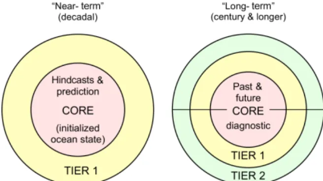
Figure 1. Predictions of interest to the Decadal Climate Predic-tion Project proceed from an initial condiPredic-tion problem at shorter timescales to a forced boundary-value problem at longer timescales (modified from Kirtman et al., 2013, Fig. 11.2).

“ability to predict” the actual evolution of the climate system. A forecast is essentially useless unless there is some indica-tion of its expected skill. A sequence of retrospective fore-casts (known as “hindfore-casts”) made with a single model, or preferably multiple models, can provide historical skill mea-sures as well as estimates of predictability. The forecasts also provide information, together with targeted simulations, for understanding the physical mechanisms that govern climate variation, and this is important for the science as well as for engendering confidence in the forecasts.

The evolution of the forecast and observed variables of the physical climate system is a combination of externally forced and internally generated components, both of which are important on annual to decadal timescales. The exter-nally forced components are the result of changes in green-house gases, anthropogenic and volcanic aerosols, variations in solar irradiance and the like. Examples of internally gen-erated variability include the El Niño–Southern Oscillation (ENSO), important on annual timescales, and the multi-year to multi-decadal variations in both the Pacific and Atlantic oceans. Decadal predictions encompass aspects of both an initial value and a forced boundary value problem as indi-cated in Fig. 1. It is important for successful decadal predic-tion that both the externally forced and internally generated components of the system are initialized, and it is also use-ful to diagnose their individual contribution to the skill of the hindcasts and forecasts.

(3)

G. J. Boer et al.: The DCPP contribution to CMIP6 3753

Figure 2.Schematic of focus areas of CMIP5 divided into prior-itized tiers of experiments (from Taylor et al., 2009). The DCPP structure is similar but consists of three focus areas (Hindcasts, Forecasts, Mechanisms), each of which is tiered as summarized in Table 1 and in the appendices as well as on the DCPP website.

2 Decadal prediction and CMIP5

While long-term climate simulations have been investigated for some time, the fifth Coupled Model Intercomparison Project (CMIP5; Taylor et al., 2012) represents one of the first attempts at a coordinated multi-model initialized decadal forecasting experiment as illustrated in Fig. 2. Results based on the hindcasts from the CMIP5 experiments have been re-ported in the literature and have contributed to Chapter 11 (Kirtman et al., 2013) of the Intergovernmental Panel on Cli-mate Change (IPCC) fifth assessment report (IPCC, 2013) entitled Near-term Climate Change: Projections and Pre-dictability. These comparatively early results indicate that there is skill in predicting the annual mean temperature evo-lution for a number of years into the future (e.g. Doblas-Reyes et al., 2013). The upper panels of Fig. 3 plot the cor-relation skill of the Year 1 and Year 2 forecasts and the Year 2–5 average forecast for surface air temperature. The impact of initialization, based on differences between uninitialized historical simulations and initialized decadal predictions, is plotted in the lower panels. The results are based on the out-put of five forecast models participating in CMIP5 (CanCM4, GFDL, MPI-ESL-LR, MIROC5, HadCM3) and the HadCM3 PPE from the ENSEMBLES project. Similar results for pre-cipitation are available but show considerably less skill at this stage. The expectation is that the improvements in the fore-cast systems participating in CMIP6 will lead to improved skill for this important parameter (Smith et al., 2012). The results in Fig. 3 are based on earlier models and approaches, but it is clear that predictions of surface air temperature have considerable skill for a number of years and for multi-year averages. The enhancement of skill due to the initialization of the forecasts is greatest in the first few years and for par-ticular regions such as the North Atlantic (as discussed under Component C) and becomes less so at longer forecast ranges where skill is provided mainly by the externally forced com-ponent.

This behaviour is seen also in Fig. 4, where the global average of the correlation skill for surface air temperature from a single model is plotted. The orange curve indicates the overall correlation skill associated with the prediction of both forced and internally generated components of variabil-ity. While the separation is approximate, the blue curve esti-mates the skill associated with the initialization of the inter-nally generated component, and the difference between the curves indicates the skill associated with the forced compo-nent. The skill of the initialized internally generated com-ponent displays classical forecast behaviour and declines to-ward zero as the forecast progresses. The externally forced component, on the other hand, maintains skill at longer cast times. The result is that the overall skill of decadal fore-casts does not decline to zero, but plateaus or even increases as forecast range increases. Finally, Fig. 4 also plots an es-timate of “potential skill”, which is the skill that the model obtains when predicting its own evolution. To the extent that the model suitably reflects the behaviour of the actual sys-tem, this at least suggests that there may be additional skill that could be accessed by the improved forecasting systems that will be used in the DCPP.

3 The DCPP and CMIP6

The approach taken in the DCPP contribution to CMIP6 dif-fers in some respects from that in CMIP5, although both cli-mate simulations and decadal hindcasts are again important components. The DCPP contribution is a CMIP6-endorsed model intercomparison project which consists of three com-ponents, each of which comprises a central “core” and ad-ditional desirable, but less central, experiments and integra-tions. Terminology has changed slightly compared to CMIP5 in Fig. 1, with core experiments now denoted as “Tier 1” and so on for the other tiers. The experience gained in CMIP5 and the subsequent improvements made in forecast systems make it timely to revisit an improved and extended decadal prediction component for CMIP6.

The lessons learned from the CMIP5 decadal prediction experiments have been incorporated into the design of the DCPP. Differences in the CMIP6 experimental protocol com-pared to that of CMIP5 include more frequent hindcast start dates and larger ensembles of hindcasts for each start date intended to provide robust estimates of skill (e.g. Sienz et al., 2016), the addition of ongoing quasi-operational experimen-tal decadal forecasts (Smith et al., 2013a), and the addition of targeted experiments to provide insight into the physical processes affecting decadal variability and forecast skill (e.g. Ruprich-Robert et al., 2016).

The three components of the DCPP are the following. – Component A, Hindcasts: the design and organization of

(4)

Figure 3.Correlation skill for Year 1, Year 2 and Year 2–5 forecasts of surface air temperature (upper panels). Impact of initialization (lower panels) based on the results from CanCM4, GFDL, MPI-ESL-LR, MIROC5, HadCM3 and the HadCM3 PPE hindcasts. Stippling denotes that the results are significant at the 10 % level (using a two-tailed test). Plots provided by R. Eade (private communication, 2016).

1 2 3 4 5 7 10

Global mean of correlation skill

Forced plus internally generated

Internally generated "P otential"

Forecast range (yr)

Figure 4.Global average correlation skill for surface air tempera-ture from a single model (based on results from Boer et al., 2013). The orange curve plots the overall skill and the blue curve the skill associated with the initialized internally generated component. The difference between the two curves is associated with the forced component. The dashed line is an estimate of the “potential” skill that could be available if the actual system operated in the same fashion as the model.

of a comprehensive archive of results for research and applications

– Component B, Forecasts: the ongoing production of experimental quasi-operational decadal climate predic-tions in support of multi-model annual to decadal

fore-casting and the application of the forecasts to societal needs

– Component C, Predictability, mechanisms, and case studies: the organization and coordination of decadal climate predictability studies and of case studies of par-ticular climate shifts and variations, including the study of the mechanisms that determine these behaviours Components A and B are directed toward the production, analysis and application of annual, multi-annual to decadal forecasts. A major output of these components is a multi-model archive of retrospective and real-time forecasts, which will serve as a resource for the analysis, understanding, and improvement of near-term climate forecasts and forecasting techniques and for their potential application (e.g. Asrar and Hurrell, 2013; Caron et al., 2015).

(5)

G. J. Boer et al.: The DCPP contribution to CMIP6 3755 The DCPP contribution to CMIP6 represents an evolution

of the design of the CMIP5 decadal prediction effort, but also, and perhaps more importantly, embodies the evolution and improvement of the components of end-to-end hindcast-ing/forecasting systems. The research and development ef-forts contributing to the DCPP include improvements in the analysis of the observations available for initializing fore-casts (e.g. Chapters 2–4, IPCC, 2013), in methods of initializ-ing models and of generatinitializ-ing ensembles of initial conditions (e.g. Balmaseda et al., 2015, and others in this Special Issue), in the representation of atmospheric, oceanic and terrestrial components of the models used in the production of the fore-casts and in their coupling (e.g. Chapter 9, IPCC, 2013), in methods of post-processing the forecasts, including new ap-proaches to bias adjustment, to calibration and multi-model combination of the forecasts, and in production and appli-cation of probabilistic decadal forecasts (e.g. Troccoli et al., 2008; Jolliffe and Stephenson, 2011). Since many of these topics have been treated fairly recently in the IPCC Fifth As-sessment Report (IPCC, 2013), for instance, we do not at-tempt to review them here. One of the goals of the DCPP is to encourage new methods and approaches to decadal fore-cast production rather than to specify rigid procedures.

4 A multi-system approach

The DCPP represents a “multi-system” approach to climate variation and prediction in which the basic experiments are specified but the details of the implementation are not. The reason for this resides in the uncertainty inherent in any cli-mate prediction or simulation. The DCPP does not specify the data or the methods to be used to initialize forecasts (e.g. full-field or anomaly initialization) or how to generate en-sembles of initial conditions. The assumption is that the dif-ferences in initializing data sets sample the uncertainty that the ensemble of initial conditions is meant to represent. The consequences of these uncertainties in initial conditions are expressed both within and across model results. Differences in model resolution and physical formulation also give rise to differences in results which are a reflection of uncertainty. A “multi-model forecast” (better a multi-system forecast) com-bines the results from forecast systems which partake of di-verse models and methods, each of which represent the “best efforts” of the modelling groups involved. The overall re-sult is increased skill (e.g. IPCC Chapter 11, DelSole et al., 2014). Differences between models may also be analyzed to understand how different formulations affect the skill of the forecasts.

As has been the case for weather and seasonal forecasting (e.g. Bauer et al., 2015; MacLachlan et al., 2015), continued improvement in each of the components of a decadal fore-casting system is expected to yield improvement in decadal prediction skill. These considerations apply also to improve-ments in the simulation and understanding of climate system

behaviour as represented by the sequence of CMIP efforts culminating in CMIP6 (Eyring et al., 2016).

5 Analysis of results

The scientific analysis of the DCPP is predicated on its broad multi-system approach. In particular, the extensive archive of multi-system results is a resource for the analysis commu-nity, and many novel and innovative analyses will be under-taken based on the availability of these data. The improve-ments in the design of the Component A hindcast exper-iment, the broader participation compared to CMIP5, and the augmented archive of results provide the basis for many types of analyses. The most obvious analysis results for Component A hindcasts are measures of historical forecast skill on annual, multi-annual and decadal forecast ranges for each system and, ultimately, for an optimum combination of these results into a multi-system forecast. The skill of the ini-tialized forecasts compared to the results of historical climate simulations is a measure of the impact of initialization and is certainly of interest. These analyses require the bias correc-tion of the forecasts, a version of which is as discussed in Appendix E. No one measure can convey all of the verifica-tion informaverifica-tion available from a set of hindcasts/forecasts (e.g. Jolliffe and Stephenson, 2011); nevertheless, there are basic measures that can be used as suggested in Goddard et al. (2013) and in the Standard Verification System for Long-range Forecasts from the World Meteorological Organization (Graham et al., 2011).

An archive of ensembles of hindcasts also permits esti-mates of the predictability, as opposed to the forecast skill, of the system and of its components (e.g. Boer et al., 2013; Hawkins et al., 2016). To the extent that the model (or multi-model combination) successfully reproduces climate system behaviour, predictability results indicate where geographi-cally, and for which variables, there may be the possibility of improving the forecast system. The overall behaviour of the forecasts and the associated predictability statistics can also reveal aspects of the mechanisms involved in governing predictability and skill as well as deficiencies in aspects of model behaviour that mitigate against skill (e.g. Eade et al., 2014).

Component B will ultimately make use of the results of Component A and together will provide research support for the eventual production of operational decadal predictions. The DCPP is an essential part of the recently established WCRP Grand Challenge of Near Term Climate Prediction (Kushnir et al., 2016). The Grand Challenge goals include the adoption of standards, verification methods and guidance for decadal predictions, the WMO recognition for operational decadal prediction and eventually the issuance of a real-time Global Decadal Climate Outlook each year.

(6)

so-called “hiatus” in global warming and the coupled AMV and IPV processes (see the entries in many chapters of IPCC, 2013). Despite these studies the processes governing these mechanisms, and their teleconnected effects, are not fully understood. The analysis of Component C archives will bring multi-system results to bear on the understanding of these mechanisms and on their effects on predictability and forecast skill. Analysis methods are being developed (e.g. Sect. 11, and references therein) where the existence of a broad archive of results offers the opportunity for new and innovative approaches.

Although episodic and of differing magnitudes, volcanic eruptions have effects on climate and on decadal predictabil-ity and skill which are of interest and importance. These are investigated in the multi-system context in Component C in collaboration with VolMIP (Zanchettin et al., 2016) and us-ing the analysis methods they suggest as well as the gen-eral approaches to skill and predictability applied to the other DCPP components.

6 DECK and CMIP6 historical simulations

The DCPP is unique in bringing together researchers from communities with expertise in seasonal to interannual pre-diction as well as climate simulation. For climate models, control and sensitivity experiments are a backdrop to climate change simulations and most models used in the DCPP will also participate in other aspects of CMIP6 and will have per-formed DECK and 20th century climate change integrations as suggested by CMIP6. Climate simulations, both equilib-rium and historical, compare ensemble and time-averaged results to the model’s equilibrium pre-industrial climate with results that are partially characterized by the models’ sensi-tivity to increasing CO2. A decadal hindcast or forecast, by

contrast, is characterized by its ability to reproduce the de-tails of system evolution on timescales of up to a decade. Results depend on the initial observation-based state, which includes system-forced climate change to that point, as well as the state of the unforced internally generated climate vari-ability. An important aspect of the analysis of results is the comparison of the forecasts with the results of historical cli-mate change simulations, with the difference representing the added information available from the initial conditions. This is another motivation for including an ensemble of historical simulations as one tier of the Component A specifications.

Comparing decadal forecasts to observations provides a different, and in some ways richer, characterization of model behaviour than is possible with the DECK results alone. For instance, Ma et al. (2014) analyze the timescale over which systematic errors develop, thus yielding insights into their origin. Also, as forecasts evolve, they lose initial condition information and approach a forced climate state giving in-formation also on this behaviour. For these reasons, while the DCPP strongly encourages participants to perform the

DECK simulations, it is recognized that this may not be fea-sible for all groups (those proposing to use high-resolution models for prediction, for instance). It is not intended that the DECK requirements should bar DCPP participation in these special cases.

7 Interactions with other MIPs

Interactions with other CMIP6 MIPs include a common ap-proach to some IPV and AMV experiments in GMMIP which will contribute to both; coordinated experiments with VolMIP with and without major volcanic forcing; outputs of DCPP hindcasts for DynVar; and the ensemble of DCPP hindcasts and simulations as contributions to DAMIP, So-larMIP and ScenarioMIP.

8 Participation

Groups are invited to participate in as many or as few of the DCPP components, each of which are separately “tiered”, as are of interest to them. The number of years of integration associated with the different tiers of each of the components and sub-components is listed in Table 1, where the different tiers are shaded. Groups are invited to consider also the Tier 4 experiments, but these are expected to be of interest to fewer groups. It is hoped that most groups will participate in the Tier 1 experiments associated with at least one of the com-ponents, but it is not expected that all groups will participate in all experiments or tiers.

9 DCPP Component A: a multi-year multi-model decadal hindcast experiment

The decadal hindcast component of CMIP follows the ex-ample of other coordinated experiments as a protocol-driven multi-model multi-national project with data production and data sharing as integral components.

The goals of the decadal hindcast component of CMIP in-clude

– the promotion of the science and practice of decadal prediction (forecasts on timescales up to and including 10 years)

– the provision of information potentially useful for the IPCC WG1 AR6 assessment report and other studies and reports on climate prediction and evolution; and – the production and retention of a year

(7)

Table 1.DCPP experiments. Table1:

Expmt experiment_id _Tier Years Description

Component A: Decadal Hindcasts

A1 dcppA-hindcast 1 3000 Five-year hindcasts every year from 1960. Note that the first forecast year is 1961 from initialization toward the end of 1960.

A2.1 2 3000 Extend A1 hindcast duration to 10 years

A2.2 dcppA-historical 2 1700 Ensemble of uninitialized historical/future simulations

A2.3 dcppA-assim 2

(60-600)

Ensemble of “assimilation” run(s) (if available). These are simulations used to incorporate observation-based data into the model in order to generate initial conditions for hindcasts. They parallel the historical simulations and use the same forcing. The number of years depends on the number of independent assimilation runs.

A3.1 dcppA-hindcast 3 300m Increase ensemble size by m for A1

A3.2 3 300m Increase ensemble size by m for A2.1

A4.1 dcppA-hindcast-niff 4 3000 As A1 but no forcing information from the future (niff) with respect to the hindcast. Forcing from persistence or other estimate.

A4.2 dcppA-historical-niff 4 3000 As A4.1 but initialized from historical simulations

Component B: Decadal Forecasts

B1 dcppB-forecast 1 50 Ongoing near-real-time forecasts

B2.1 2 5m Increase ensemble size by m for B1

B2.2 2 50 Extend forecast duration to 10 years for B1

Component C: Hiatus+

C1.1 dcppC-atl-control 1 250 Idealized Atlantic control

C1.2 dcppC-amv-pos 1 250 Idealized impact of AMV+

C1.3 dcppC-amv-neg 1 250 Idealized impact of AMV-

C1.4 dcppC-pac-control 1 100 Idealized Pacific control

C1.5 dcppC-ipv-pos 1 100 Idealized impact of IPV+

C1.6 dcppC-ipv-neg 1 100 Idealized impact of

IPV-C1.7 dcppC-amv-ExTrop-pos dcppC-amv-ExTtrop-neg

2 500 Idealized impact of extratropical AMV+ and AMV-

C1.8 dcppC-amv-Trop-pos dcppC-amv-Trop-neg

2 500 Idealized impact of tropical AMV+ and AMV-

C1.9 dcppC-ipv-NexTrop-pos dcppC-ipv-NexTtrop-neg

2 200 Idealized impact of northern extratropical IPV+ and IPV-

C1.10 dcppC-pac-pacemaker 3 650 Pacemaker Pacific experiment

C1.11 dcppC-atl-pacemaker 3 650 Pacemaker Atlantic experiment Component C:

Atlantic gyre

C2.1 dcppC-atl-spg 3 200-400 Predictability of 1990s warming of Atlantic gyre

C2.2 3 200-400 Additional start dates

Component C: Volcano

C3.1 dcppC-hindcast-noPinatubo 1 50-100 Repeat 1991 hindcast but without Pinatubo forcing

C3.2 dcppC-hindcast-noElChichon 2 50-100 Repeat 1982 hindcast but without El Chichon forcing

C3.3 dcppC-hindcast-noAgung 2 50-100 Repeat 1963 hindcast but without Agung forcing

C3.4 dcppC-forecast-addPinatubo 1 50-100 Repeat 2015 forecast with added Pinatubo forcing

C3.5 dcppC-forecast-addElChichon 3 50-100 Repeat 2015 forecast with added El Chichon forcing

C3.6 dcppC-forecast-addElChichon 3 50-100 Repeat 2015 forecast with added Agung forcing

(8)

– a system view (data; analyses; initial conditions; ensem-ble generation; models and forecast production; post-processing and assessment) of decadal prediction; – the investigation of broad questions (e.g. sources and

limits of predictability, current abilities with respect to decadal prediction, potential applications);

– the provision of benchmarks against which to compare improvements in forecast system components and their contribution to prediction quality; and

– information on processes and mechanisms of interest (e.g. the hiatus, climate shifts, Atlantic meridional over-turning circulation (AMOC), etc.) in a collection of hindcasts.

Practical aspects of Component A include

– the coordination of efforts based on agreed experimental structures and timelines in order to promote research, intercomparison, multi-model approaches, applications, and new research directions; and

– a contribution to the development of infrastructure, in particular a multi-purpose data archive of decadal hind-casts useful for a broad range of scientific and appli-cation questions and of benefit to national and interna-tional climate prediction and climate services organiza-tions.

The basic elements of Component A are

– a coordinated set of multi-model multi-member ensem-bles of retrospective forecasts initialized each year from 1960 to the present; and

– the resulting archive of forecast results generally and readily available to the scientific and applications com-munities via the Earth System Grid Federation (ESGF). Consultation and timing for Component A

– The proposed timing for Component A generally fol-lows that outlined for CMIP6 (Eyring et al., 2016). In particular, the availability of historical forcing and fu-ture scenario information is key to DCPP timing. Details of the proposed Component A decadal prediction hindcasts are listed in Appendix A.

10 DCPP Component B: experimental real-time multi-model decadal predictions

The real-time decadal prediction component of the DCPP also follows the example of other coordinated experiments as a protocol-driven multi-model multi-national project with data production and data sharing as integral components. The WMO structure already in place for seasonal forecasts is

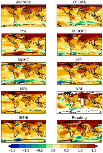
Figure 5. Example real-time multi-model decadal predictions (Smith et al., 2013a, available from http://www.metoffice. gov.uk/research/climate/seasonal-to-decadal/long-range/

decadal-multimodel). Maps show predicted near-surface tem-perature anomalies (◦C) relative to the average over 1971 to 2000 for the 5-year period 2015–2019 from forecasts starting at the end of 2014.

(9)

(a)

(b)

(c) (d)

°

° ° ° ° °

°

° ° ° ° ° ° ° ° ° °

° ° °

Figure 6.Idealized Atlantic SST patterns. The time series (upper panel) and pattern (middle panel) are derived following the procedure documented in Ting et al. (2009) using ERSSTv4 (Huang et al., 2015) as discussed in Technical Note 1 (available from the DCPP website at http://www.wcrp-climate.org/dcp-overview). Experiments C1.1 to C1.3 use the total AMV pattern (middle panel), whereas experiments C1.7 and C1.8 apply anomalies in the northern extra-tropics and tropics separately (lower panels).

GFCS and will fill a gap between seasonal predictions and long-term climate change projections.

Goals:

– as for Component A but with the added dimension that the goals apply to quasi-operational real-time multi-model decadal predictions

Scientific aspects:

– the assessment of decadal predictions of key variables, including surface temperature, precipitation, mean sea level pressure, AMV, IPV, Arctic sea ice, the North At-lantic Oscillation (NAO), and tropical storms

– the assessment of uncertainties and the generation of a consensus forecast

– the assessment of decadal predictions and associated climate impacts of societal relevance

Basic elements:

– an ongoing coordinated set of model multi-member ensembles of real-time forecasts, updated each year;

– an associated hierarchy of data sets of results gener-ally and readily available to the scientific and applica-tions communities, including National Meteorological and Hydrological Services and Regional Climate Cen-tres.

Details of the proposed Component B real-time decadal pre-diction component are listed in the Appendix B.

11 DCPP Component C: Predictability, mechanisms and case studies

(10)

(a)

(b) _(c)Year

°

° ° ° ° ° ° ° °

° ° °

° ° ° ° ° ° °

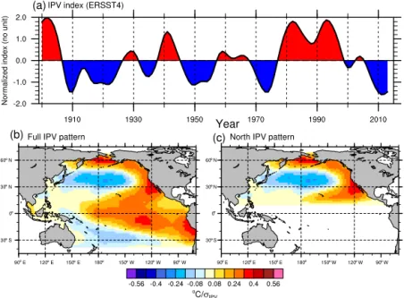
Figure 7. Idealized Pacific SST patterns. The time series (upper panel) and pattern (lower panel) are derived following the procedure documented in Ting et al. (2009) using ERSSTv4 (Huang et al., 2015) as discussed in Technical Note 1 (available from the DCPP website at http://www.wcrp-climate.org/dcp-overview). Experiments C1.4 to C1.6 use the full IPV pattern (lower left panel), whereas experiment C1.9 applies the anomalies in the northern extra-tropics (lower right panel).

Case studies are hindcasts which focus on a particular cli-matic event and the mechanisms and impacts involved. These are typically hindcast studies of an observed event, although they can include particular kinds of events seen in model inte-grations (variations of AMOC and the associated variation of the North Atlantic sea surface temperatures (SSTs) in mod-els are examples). Studies of the skill with which a particular event (e.g. the hiatus, climate shift, an extreme year) can be forecast and the mechanisms which support (or perhaps make difficult) a skilful prediction are all of interest.

The DCPP and the CLIVAR Decadal Climate Variability and Predictability (DCVP) focus group are proposing co-ordinated multi-model investigations of a limited number of mechanism/predictability/case studies believed to be of broad interest to the community. Two research areas are the current foci of Component C. They are

– Hiatus+: this is used as a shorthand to indicate investi-gations into the origins, mechanisms and predictability of long timescale variations in both global mean surface temperature (and other variables) and regional imprints, including periods of both enhanced global warming and cooling with a focus on the most recent slowdown that began in the late 1990s.

– Volcanoes in a prediction context: an investigation of the influence and consequences of volcanic eruptions on decadal prediction and predictability

Full details of the proposed experiments are given in Ap-pendix C.

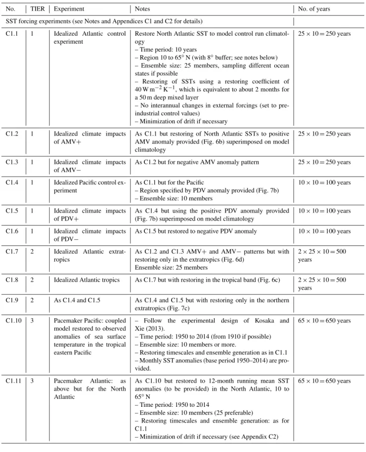
The proposed experiments in Table C1 of Appendix C are intended to discover how models respond to imposed slowly evolving SST anomalies in the Atlantic and the Pa-cific, which are perceived as originating in ocean heat con-tent or heat transport convergence anomalies. The questions at issue are the consistency of models’ responses to these SSTs and the pathways through which the responses are ex-pressed throughout the ocean and atmosphere. The experi-ments are expected to illuminate model behaviour on decadal timescales and possible mechanistic links to retarded and ac-celerated global surface temperature variations and regional climate anomalies, in other words, the extent to which modu-lations of global mean surface temperatures can be attributed to ocean heat content variations, what the respective roles of Atlantic and Pacific SST anomalies in these changes are, and to what extent we can attribute decadal climate anomalies at regional scales (particularly over land) to the patterns of At-lantic Multidecadal Variability (AMV) and Pacific Decadal Variability (PDV) sea surface temperature that are illustrated in Figs. 6 and 7. These experiments also address the interre-lationships between the AMV and PDV shifts and the mech-anisms at play.

(11)

G. J. Boer et al.: The DCPP contribution to CMIP6 3761 et al., 2010). The proposed experiments will investigate in

more detail the role of initialization of the Atlantic subpolar gyre. Analysis of these experiments will include assessment of the role of the Atlantic Meridional Overturning Circula-tion (AMOC) in the subpolar gyre warming and the impact of the subpolar gyre on the AMV pattern and associated climate impacts, including rainfall over the Sahel, Amazon, USA and Europe, and Atlantic tropical storms.

The final set of Component C experiments in Table C3 of Appendix C is jointly proposed with VolMIP (Zanchet-tin et al., 2016) and is directed toward an understanding of the effects of volcanoes on past and potentially on future decadal predictions. Removing the forcing due to major vol-canic eruptions from hindcasts during which they occurred and introducing volcanic forcing into forecasts during which no volcano occurred will allow estimates of the impact on skill to be made (e.g. Maher et al., 2015; Meehl et al., 2015; Timmreck et al., 2016). Comparing the effects of the same eruption in hindcasts and forecasts also allows the impact of the background climate state to be assessed. In addition to assessing the radiative effects arising from the aerosol load-ing in the stratosphere, an important aspect of the analysis of these experiments will be to investigate subsequent dynam-ical responses, including, for example, those involving the NAO and ENSO.

Participants are invited to undertake as many or as few of the Component C experiments as are of interest to them. Please see the Notes at the end of Appendix C for additional details on the Component C experimental protocol.

12 Concluding comments

The DCPP is unique in bringing together researchers from communities with expertise in seasonal to interannual predic-tion (as represented by WGSIP), climate simulapredic-tion (as rep-resented by WGCM), and decadal variability and predictabil-ity in general (as represented by CLIVAR). The models used and approaches taken represent to varying degrees the inter-ests and abilities of these communities.

For climate models, control and sensitivity experiments are a necessary backdrop to climate change simulations. Most models used in the DCPP will also participate in other aspects of CMIP6 and will have performed climate integra-tions as well as other simulaintegra-tions and MIP experiments. The data retained for these studies provide information on forced responses and the statistics of internal variability which are important for DCPP-related studies of many different as-pects of decadal variability and prediction. The forecasting aspect of DCPP encourages emphasis on methods of initial-izing models, generating ensembles of forecasts and, espe-cially, on assessing results against observations. The two ap-proaches represent complementary views of the understand-ing and prediction of forced and internally generated climate variations. The tiered set of retained data for the DCPP is

intended to assist in the evaluation and analysis of DCPP results, but groups are encouraged to retain additional data relevant to other MIPs if possible.

We believe that the Decadal Climate Prediction Project represents an important evolutionary advance from the CMIP5 decadal prediction component and addresses an inte-grated range of scientific issues broadly characterized as the ability of the system to be predicted on decadal timescales, the currently available skill, the mechanisms that control long timescale variability, and the ongoing production of forecasts of potential benefit for both science and societal applications. This will be a major resource to support the WCRP’s new Grand Challenge of Near Term Climate Prediction and an important asset for the development of climate services on timescales relevant to a wide range of users.

13 Data availability

The model output from DCPP hindcasts, forecasts, and tar-geted experiments described in this paper will be distributed through the Earth System Grid Federation (ESGF) with digi-tal object identifiers (DOIs) assigned. The list of requested variables, including frequencies and priorities, is given in Appendix D and has been submitted as part of the CMIP6 Data Request Compilation. As in CMIP5, the model output will be freely accessible through data portals after a sim-ple registration process that is unique to all CMIP6 compo-nents. In order to document CMIP6’s scientific impact and enable ongoing support of CMIP, users are requested to ac-knowledge CMIP6, the participating modelling groups, and the ESGF centres (see details on the CMIP website). Fur-ther information about the infrastructure supporting CMIP6, the metadata describing the model output, and the terms gov-erning its use is provided by the WGCM Infrastructure Panel (WIP). Links to this information may be found on the CMIP6 website and are discussed in the WIP contribution to this Special Issue. Along with the data themselves, the prove-nance of the data will be recorded, and DOIs will be as-signed to collections of output so that they can be appropri-ately cited. This information will be made readily available so that research results can be compared and the modelling groups providing the data can be credited.

(12)

Appendix A: Component A hindcasts

The approach parallels that of the “Near-term Decadal” com-ponent of CMIP5 (Taylor et al., 2009), with important dif-ferences, notably that the hindcasts are to be produced ev-ery year, rather than evev-ery 5 years. As noted previously, “decadal” and “near-term” are used here to indicate annual, multi-annual and up to 10-year hindcasts. The Tier 1 exper-iment consists of hindcasts for years 1–5 for which the im-pact of initialization is expected to be greatest. Forecast skill is not geographically uniform and some regions will exhibit skill on longer timescales. The A2.1 experiment extends the hindcasts to years 6–10 to allow for the identification of these regions when resources permit. The A2.2 uninitialized histor-ical simulations are compared with the initialized forecast to assess the impact of initialization.

Table A1 lists the main DCPP Component A experi-ments. The A1 hindcast experiment parallels the correspond-ing CMIP5 decadal prediction experiment in uscorrespond-ing the same specified forcing as is used for the CMIP6 historical climate simulations. This forcing is also used for the historical sim-ulations of experiment A2. For forecasts which extend be-yond the period for which historical forcing is specified, the “medium” SSP2-4.5 forcing of ScenarioMIP (O’Neill et al., 2016) is used. This forcing scenario is used for several other MIPs and is chosen since “land use and aerosol pathways are not extreme relative to other SSPs (and therefore appear as central for the concerns of DAMIP and DCPP), and also be-cause it is relevant. . . as a scenario that combines intermedi-ate societal vulnerability with an intermediintermedi-ate forcing level”. This forcing is also used for experiment A2.2, which is also a contribution to ScenarioMIP.

The specification of historical forcing introduces some in-formation from the future with respect to the forecast and may lead to slightly overestimated historical forecast skill measures. The main effect is expected to be due to the spec-ification of short-term radiative forcings such as volcanoes which occur during a forecast. Other forcings, such as those associated with greenhouse gas and aerosol emissions and/or concentrations, vary comparatively slowly over the 5- or 10-year period of a forecast and are expected to have little effect on the results. The benefits of using specified forcings in-clude the use of common values across models, the ease of treatment within models, the possibility of documenting im-provements with respect to CMIP5 hindcasts, the ability to estimate the effects of initialization by comparing forecasts and simulations which use the same forcings, and the esti-mation of drift corrections from hindcasts which include the forcings and so are more suitable for the purpose of future decadal forecasts.

Component A benefits from and builds on the experi-ence gained from the decadal component of CMIP5. It calls for hindcasts every year, rather than every 5 years, which will improve the statistical stability of results, allow more sophisticated drift treatments, more clearly delineate skill levels, and foster improved assessment, combination, and calibration of the forecasts. Broad participation in Compo-nent A will potentially allow classification of results accord-ing to (i) the initialization of climate components in the mod-els, (ii) model resolutions including atmospheric model top, and (iii) methods of initialization and ensemble generation. DCPP component A also provides an opportunity to study solar effects on climate. In order to take advantage of this, however, groups should use the correct ozone forcing time series which is important for the impact of solar variations.

Table A2 lists additional experiments which are of interest if resources permit. The Tier 3 experiments, A3.1 and A3.2, increase the ensemble size in order to better isolate the pre-dictable component in the case of a deterministic forecast and to better represent the probability distribution in the case of a probabilistic forecast. The A3 experiments may be used to help quantify the benefits of larger ensembles as a guide to future forecast applications. In the Tier 4 hindcasts the ex-ternal forcing applied is based on information available at the start of the forecast (using persistence, extrapolation, or some other method). This contrasts with the Tier 1 hindcasts where historical forcings are applied as discussed above. It is not expected that many groups will undertake the Tier 4 experiments, which require an additional large commitment of resources. They are included for completeness and in case the needed resources become available.

(13)

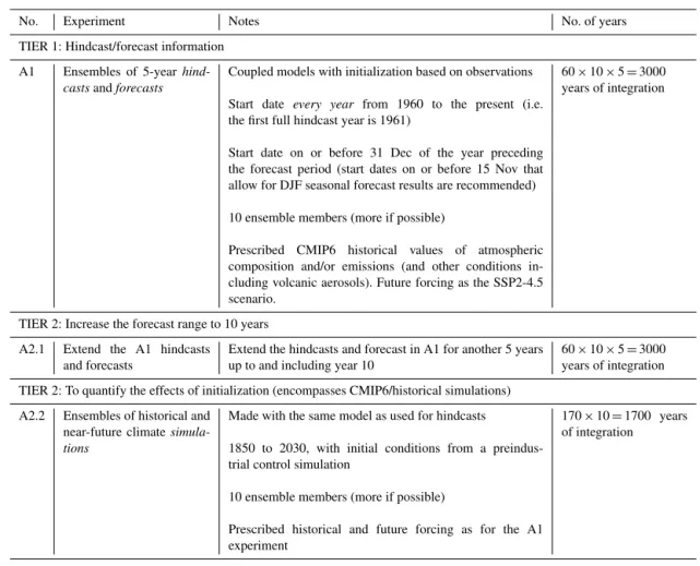
Table A1.Basic Component A: Hindcast/forecast experiments.

No. Experiment Notes No. of years

TIER 1: Hindcast/forecast information A1 Ensembles of 5-year

hind-castsandforecasts

Coupled models with initialization based on observations Start date every year from 1960 to the present (i.e. the first full hindcast year is 1961)

Start date on or before 31 Dec of the year preceding the forecast period (start dates on or before 15 Nov that allow for DJF seasonal forecast results are recommended) 10 ensemble members (more if possible)

Prescribed CMIP6 historical values of atmospheric composition and/or emissions (and other conditions in-cluding volcanic aerosols). Future forcing as the SSP2-4.5 scenario.

60×10×5=3000 years of integration

TIER 2: Increase the forecast range to 10 years A2.1 Extend the A1 hindcasts

and forecasts

Extend the hindcasts and forecast in A1 for another 5 years up to and including year 10

60×10×5=3000 years of integration TIER 2: To quantify the effects of initialization (encompasses CMIP6/historical simulations)

A2.2 Ensembles of historical and near-future climate simula-tions

Made with the same model as used for hindcasts

1850 to 2030, with initial conditions from a preindus-trial control simulation

10 ensemble members (more if possible)

Prescribed historical and future forcing as for the A1 experiment

170×10=1700 years of integration

Table A2.Other hindcast experiments (if resources permit).

TIER 3: Effects of increased ensemble size A3.1 Increased ensemble size for

the A1 experiment

madditional ensemble members to improve skill and exam-ine dependence of skill on ensemble size

60×5×m=300m years of integration A3.2 Increased ensemble size for

the A2 experiment

As A3.1 but for the A2.1 experiment 60×5×m=300m years of integration TIER 4: Improved estimates of hindcast skill

A4.1 Ensembles of at least 5-year, but much preferably 10-year, hindcasts and fore-casts

As A1 but with no information from the future with respect to the forecast

Radiative and other forcing information (e.g. green-house gas concentrations, aerosols) maintained at the initial state value or projected in a simple way. No inclusion of volcano or other short-term forcing unless available at the initial time.

3000–6000 years of integration

TIER 4: Improved estimates of the effects of initialization A4.2 Ensembles of at least

5-year, but much preferably 10-year, hindcasts and fore-casts

Historical climate simulations up to the start dates of corresponding forecast with prescribed forcing

Simulations continued from forecast start date but with the same forcing as in A4.1, i.e. with NO forcing information from the future with respect to the start date. These are uninitialized versions of A4.1 hindcasts.

(14)

Appendix B: Component B: forecasts Objective:

– Production, collection and combination of real-time quasi-operational decadal forecasts

Explanatory comment

Component B real-time decadal forecasts are currently be-ing produced based on CMIP5 and usbe-ing other models and hindcast data sets. The intent is that the forecasts produced by these models will be augmented by Component A results as they become available. Data to be retained on the ESGF are the same as listed in the DCPP Data Retention Table in Appendix D. Data to be archived by 31 January of each year if possible.

Table B1.Real-time decadal forecasts.

TIER 1: Real-time forecasts

B1 Ensembles of ongoing real-time 5-year forecasts

Coupled models with initialization based on observations

Start dateevery yearongoing

Start date on or before 31 Dec (start dates on or be-fore 15 Nov allow for DJF seasonal be-forecast results and are recommended)

10 ensemble members (more if possible)

Atmospheric composition and/or emissions (and other conditions including volcanic aerosols) to follow a prescribed forcing scenario as in A1.

10×5=50 years of integration for 5-year forecasts

TIER 2: Increased ensemble size and duration

B2.1 Increase ensemble size madditional ensemble members to reduce noise and im-prove skill

5myears of integration

B2.2 Extend forecast duration to 10 years

To provide forecast information for the period 5 to 10 years ahead

(15)

G. J. Boer et al.: The DCPP contribution to CMIP6 3765 Appendix C: Component C: Predictability,

mechanisms, and case studies

Component C consists of targeted simulations and predic-tion intended to (i) investigate the origins, mechanisms and predictability of long timescale variations in climate as well as their regional imprints and (ii) to investigate the influence and consequences of volcanic eruptions on decadal predic-tion and predictability. See the Notes for details on methods and data.

Component C1: accelerated and retarded rates of global temperature change and associated regional climate variations (Table C1)

Objective:

– to investigate the role of eastern and North Pacific and North Atlantic SSTs in the modulation of global surface temperature trends and in driving regional climate vari-ations.

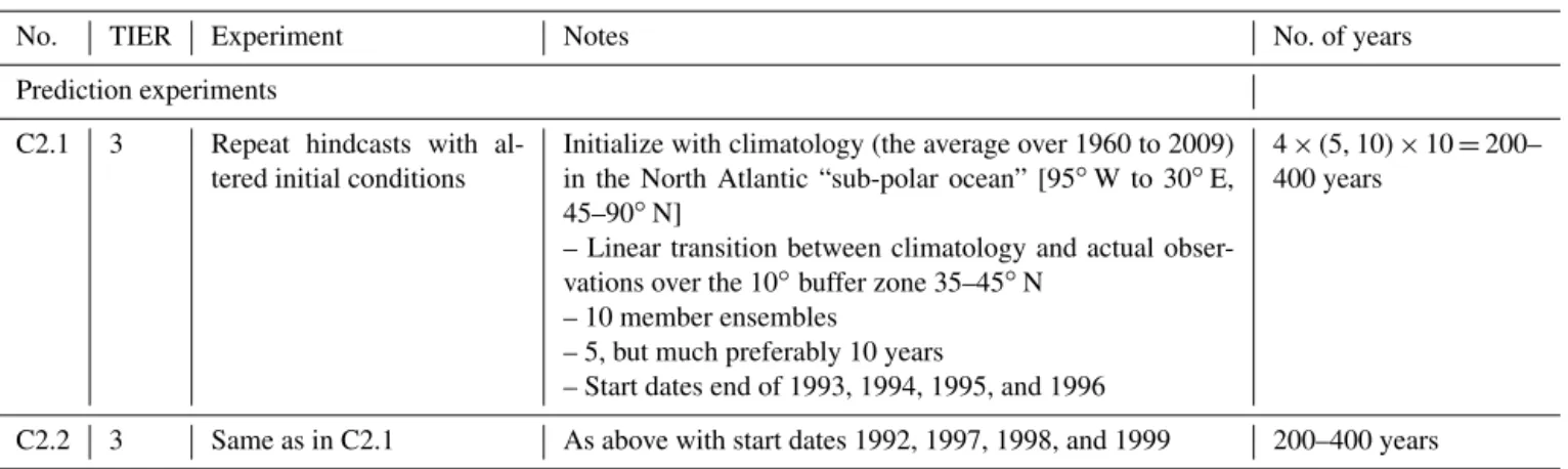
Component C2: Case study of mid-1990s Atlantic subpolar gyre warming (Table C2)

Objectives:

– to investigate the predictability of the mid-1990s warm-ing of the subpolar gyre and its impact on climate vari-ability.

Component C3: Volcano effects on decadal prediction (Table C3)

Objectives:

– Assess the impact of volcanoes on decadal prediction skill.

– Investigate the potential effects of a volcanic eruption on forecasts of the coming decade.

– Investigate the sensitivity of volcanic response to the state of the climate system.

Notes

Experiments C1.1–1.9 are idealized coupled model exper-iments following the methodology described in Ruprich-Robert et al. (2016) but with some changes. The AMV and IPV patterns used are displayed in Figs. 6 and 7. The pat-terns are derived from the difference between observations and the ensemble mean of coupled model historical simu-lations (Ting et al., 2009) and are an estimate of unforced

internal variability. Although this estimate is not perfect be-cause the modelled response to external factors such as an-thropogenic aerosols may not be entirely correct, the exper-iments nevertheless provide information on the climate re-sponse to North Atlantic and Pacific SST variations. The ex-periments are based on model control integrations rather than historical simulations and therefore may be performed be-fore the updated CMIP6 forcings become available. See the DCPP website (http://www.wcrp-climate.org/dcp-overview) for links to Technical Note 1, which documents the methods used to produce the AMV and IPV patterns, and for links to the SST data to be used in the experiment.

Experiments C1.10 and C1.11 follow the design of Kosaka and Xie (2013) in which observed SST anomalies are im-posed in the tropical Pacific region in coupled model simula-tions. The results will be compared to the standard historical simulations to infer the impact of the tropical Pacific SSTs.

These “pacemaker” experiments (C1.10 and C1.11) are of considerable interest in a multi-model context in which the response of the models to SSTs, imposed in the man-ner of Kosaka and Xie (2013), is considered. Questions in-clude the robustness of the results across models, the geo-graphic and global effects on climate and the pathways in the ocean and atmosphere through which the forcing is ex-pressed. The experiments are Tier 3, however, because there may be coupled adjustment and drift issues that affect the re-sults, and this should be considered before undertaking the experiments. These include drift minimization (see below) and differences in variance and seasonality between models and observations. For these experiments,

– observed monthly SST anomalies (base period 1950– 2014) are superimposed onto the model climatol-ogy over the same period computed from histori-cal simulations in order to minimize model drift. See the DCPP website (http://www.wcrp-climate.org/ dcp-overview) for links to these data.

– Experiments should cover the period from 1950 to 2014, but starting from 1910 is desirable if possible.

– External forcings as for historical simulations

Methods of constraining SSTs and minimizing drifts are dis-cussed in Technical Note 2 (available from the DCPP website at http://www.wcrp-climate.org/dcp-overview).

– The SST signal is imposed either by altering surface fluxes or by restoring the SST directly with no restor-ing if sea ice is present. Outside of the restorrestor-ing region, the model evolves freely, allowing a full climate system response.

(16)

Table C1.Accelerated and retarded rates of global temperature change and the associated regional climate variations.

No. TIER Experiment Notes No. of years

SST forcing experiments (see Notes and Appendices C1 and C2 for details)

C1.1 1 Idealized Atlantic control experiment

Restore North Atlantic SST to model control run climatol-ogy

– Time period: 10 years

– Region 10 to 65◦N (with 8◦buffer; see notes below) – Ensemble size: 25 members, sampling different ocean states if possible

– Restoring of SSTs using a restoring coefficient of 40 W m−2K−1, which is equivalent to about 2 months for a 50 m deep mixed layer

– No interannual changes in external forcings (set to pre-industrial control values)

– Minimization of drift if necessary

25×10=250 years

C1.2 1 Idealized climate impacts of AMV+

As C1.1 but restoring of North Atlantic SSTs to positive AMV anomaly provided (Fig. 6b) superimposed on model climatology

25×10=250 years

C1.3 1 Idealized climate impacts of AMV−

As C1.2 but for negative AMV anomaly pattern 25×10=250 years

C1.4 1 Idealized Pacific control ex-periment

As C1.1 but for the Pacific

– Region specified by PDV anomaly provided (Fig. 7b) – Ensemble size: 10 members

10×10=100 years

C1.5 1 Idealized climate impacts of PDV+

As C1.4 but using the positive PDV anomaly provided (Fig. 7b) superimposed on model climatology

10×10=100 years

C1.6 1 Idealized climate impacts of PDV−

As C1.5 but restored to negative PDV anomaly 10×10=100 years

C1.7 2 Idealized Atlantic extrat-ropics

As C1.2 and C1.3 AMV+and AMV−patterns but with restoring only in the extratropics (Fig. 6d)

Ensemble size: 25 members

2×25×10=500 years

C1.8 2 Idealized Atlantic tropics As C1.7 but with restoring in the tropical band (Fig. 6c) 2×25×10=500 years

C1.9 2 As C1.4 and C1.5 As C1.4 and C1.5 but with restoring only in the northern extratropics (Fig. 7c)

C1.10 3 Pacemaker Pacific: coupled model restored to observed anomalies of sea surface temperature in the tropical eastern Pacific

– Follow the experimental design of Kosaka and Xie (2013).

– Time period: 1950 to 2014 (from 1910 if possible) – Ensemble size: 10 members or more.

– Restoring timescales and ensemble generation as in C1.1 – Monthly SST anomalies (base period 1950–2014) are pro-vided.

65×10=650 years

C1.11 3 Pacemaker Atlantic: as above but for the North Atlantic

As C1.10 but restored to 12-month running mean SST anomalies (to be provided) in the North Atlantic, 10 to 65◦N

– Time period: 1950 to 2014

– Ensemble size: 10 members (25 preferable)

– Restoring timescales and ensemble generation: as for C1.1

– Minimization of drift if necessary (see Appendix C2)

(17)

Table C2.Case study of mid-1990s Atlantic subpolar gyre warming.

Prediction experiments

C2.1 3 Repeat hindcasts with al-tered initial conditions

Initialize with climatology (the average over 1960 to 2009) in the North Atlantic “sub-polar ocean” [95◦W to 30◦E, 45–90◦N]

– Linear transition between climatology and actual obser-vations over the 10◦buffer zone 35–45◦N

– 10 member ensembles

– 5, but much preferably 10 years

– Start dates end of 1993, 1994, 1995, and 1996

4×(5, 10)×10=200– 400 years

C2.2 3 Same as in C2.1 As above with start dates 1992, 1997, 1998, and 1999 200–400 years

Table C3.Volcano effects on decadal prediction.

Prediction experiments with and without volcano forcing

C3.1 1 Pinatubo Repeat 1991 hindcasts without Pinatubo forcing. – 5-year, but preferably 10-year, hindcasts – 10 ensemble members

– Specify the “background” volcanic aerosol to be the same as that used in the 2015 forecast

(5 or 10)×10=50– 100 years

C3.2 2 El Chichon 1982 hindcasts as above but without El Chichon forcing 50–100 years

C3.3 2 Agung 1963 hindcasts as above but without Agung forcing 50–100 years

Prediction experiments for 2015 with added forcing

C3.4 1 Added forcing Repeat 2015–2019/24 forecast with Pinatubo forcing. 50–100 years

C3.5 3 Added forcing Repeat 2015–2019/24 forecast with El Chichon forcing. 50–100 years

C3.6 3 Added forcing Repeat 2015–2019/24 forecast with Agung forcing. 50–100 years

South Atlantic) and which can obscure the results. It is recommended that groups monitor this potential re-sponse and take steps to minimize it, if necessary fol-lowing the recommendations in Technical Note 2. – In order to sample uncertainties in the ocean initial state,

it is recommended that, if possible, ensemble members are generated by taking initial conditions from differ-ent members of the historical simulations. Otherwise, ensembles may be generated by perturbing atmospheric conditions.

(18)

Appendix D: DCPP Data Retention Tables

The DCPP is concerned with prediction and a main interest is in variables that can be verified against observations. Vari-ables that provide insight into the ability to predict observed behaviour and the mechanisms involved are, of course, also of interest. There is a somewhat different emphasis on re-tained variables for the DCPP compared to the more usual approach which aims to study budgets, balances, processes, etc. in the context of climate simulation rather than pre-diction. The large number of forecast years involved in the DCPP is also a consideration.

We stress that the DCPP Data Retention Tables are not intended to excludeother variables. If modelling groups are willing and able to retain the variables requested by other MIPs, also for the DCPP, this would be ideal.

The following is intended as a prioritized set of variables for verification and investigation, but isnot intended to re-strictthe amount of data that groups retain for their DCPP integrations. With this understanding, the DCPP list is or-dered into priorities as follows.

– Priority 1. These are basic forecast variables aimed at permitting bias adjusted forecast assessment, especially of well-observed surface parameters and some atmo-spheric and oceanic structures, together with data that provide some information on the budgets and balances involved.

– Priority 2. These are important variables that allow more detailed forecast assessment including, to some extent, predictions for the body of the atmosphere and ocean. – Priority 3. These variables are intended for special

in-terest investigations.

Participants should strive to retain at least Priority 1 vari-ables and also Priority 2 varivari-ables to the extent that this is possible. Some basic discussion and recommendations on bias adjustment are given in Appendix E.

These tables are intended to provide an overview. De-tailed specifications, including units, etc., will be part of the “CMIP6 Data Request Compilation”.The table headings in-dicate the nature of the data (e.g. TOA and BOA inin-dicate top or bottom of the atmosphere) and the averaging period, yearly, monthly, daily or 6 h sampling. We have attempted to use standard CMIP5 variable names throughout, although it is possible that there could be some differences with the CMIP6 Data Request Compilation.

Special data sets for consideration in support of other MIPs

(19)

Table D1.DCPP Data Retention Table.

CMIP5 name Short description Averaging or sampling

period and priority Yr Mon Day 6 h

TOA fluxes

rsdt solar incident 1 3

rsut solar out 1 3

rlut lw out 1 3

rsutcs clear sky solar out 2

rlutcs clear sky lw out 2

2-D atmosphere and surface variables

tas sfc airT 1 1 2

tasmax dayT max 1 1

tasmin dayT min 1 1

uas EW wind 1 2 2

vas NS wind 1 2 2

sfcWind day mean wind 1 1

sfcWindmax day max wind 1 1

huss specific humidity 1

tdps dewpoint temp 2 2

clt cld frac 1 2

ps sfc pres 2

psl mean sea level pressure 1 1 2

Other high-frequency data

zg1000 1000 hPa geopotential 2

rv850 850 hPa relative vorticity 3

BOA fluxes

rsds solar down 1 1

rlds LW down 3 3

rss net solar 1 3

rls net LW 1 3

tauu EW stress down 2 3

tauv NS stress down 2 3

hfss sensible up 1 3

hfls latent up 1 3

evspsbl net evap 1

pr net pcp 1 1 2

prsn pcp as sno 3 3

prhmax day max hourly pcp 1 1 3

Land

Physical variables

ts skin temp 1

alb sfc albedo 1

mrso soil moist 1 3

mrfso frozen soil moist 1

snld sno depth 1 3

(20)

Table D1.Continued.

Land

Biogeophysical variables

treeFrac tree fraction 2

grassFrac grass fraction 2

shrubFrac shrub fraction 2

cropFrac crop fraction 2

vegFrac total vegetated fraction 2

baresoilFrac bare soil fraction 2

residualFrac residual land fraction 2

cVeg vegetation carbon content 2

cLitter litter carbon content 2

cSoil soil carbon content 2

cProduct carbon content of products of anthropogenic land use change

2

cLand total land carbon 2

netAtmosLandCO2Flux net atmosphere to land CO2flux 2

gpp gross primary productivity 2

npp net primary productivity 2

lai leaf area index 2

nbp surface net downward mass flux of CO2as

car-bon due to all land processes

2

rh heterotrophic respiration carbon flux 2

ra plan respiration carbon flux 2

Sea Ice

tsice sfc temp 3 3

sic ice fraction 1 3

sit ice thickness 1

snld sno thickness 2 3

hflssi latent heat flux up 3

hfssi sensible heat flux up 3

usi EW ice speed 3

vsi NS ice speed 3

strairx EW stress down 3

strairy NS stress down 3

2-D Ocean (preferably on regular grid)

tos SST 1

sos SSS 2

t20d depth 20◦C 1 2

mlotst thickness mix layer 1 2

thetaot depth avg pot temp 1

thetao300 depth avg pot temp to 300 m 1

thetao700 700 m 1

thetao2000 2000 m 1

msftmyz MOC 1

(21)

Table D1.Continued.

2-D Ocean (preferably on regular grid)

hfnorth northward ocean heat transport 2

hfbasin northward ocean heat transport 2

sltnorth northward ocean salt transport 2

sltbasin northward ocean salt transport 2

zos sea sfc height 1

zossq square sea sfc height 2

zostoga thermosteric sea level change 2

volo volume of seawater 2

hfds net heat into ocean 1

vsf virtual salt into ocean (or equivalent freshwater flux)

1

Biogeochemical variables (for ESMs)

intpp primary production 2

epc100 downward flux of particle organic carbon 2

epcalc100 CaCO3export at 100 m 2

epsi100 opal export at 100 m 2

spco2 surface aqueous partial pressure of CO2 2

fgco2 surface downward CO2flux 2

co2s atmospheric CO2 2

3-D Atmos (850, 500, 200, 100, 50) Priority 1 (925, 700, 300, 30,20, 10) Priority 2

Note that these levels may change based on future review.

ta temp 1

ta850 temp 850 1

ua EW wind 1

va NS wind 1

hus spec hum 2

zg geopotential 1

zg500 geopotential 500 1

wap vertical press velocity 2

3-D Ocean (preferably on a regular grid at standard levels)

thetao pot temp 2

so salt 2

uo EW speed 2

vo NS speed 2

wo upward speed 3

Biogeophysical variables (for ESMs)

dissic dissolved inorganic carbon concentration 2 dissoc dissolved organic carbon concentration 2

talk total alkalinity 2

(22)

Table D1.Continued.

3-D Ocean (preferably on a regular grid at standard levels)

Biogeophysical variables (for ESMs)

o2 dissolved oxygen concentration 2

phyc phytoplankton carbon concentration 2

chl total chlorophyll mass concentration 2

zooc zooplankton carbon concentration 2

ph seawater pH (reported on the total scale) 2 pp total primary (organic carbon) production by

phytoplankton

2

nh4 dissolved ammonium concentration 2

po4 dissolved phosphate concentration 2

dfe dissolved iron concentration 2

si dissolved silicate concentration 2

expc sinking particulate organic carbon flux 2 zfull depth below geoid of ocean layer 2

(23)

G. J. Boer et al.: The DCPP contribution to CMIP6 3773 Appendix E: Bias correction for decadal climate

predictions Introduction

No model is perfect and the result is a difference, or bias, be-tween simulated and observed climatologies. This bias may introduce errors into a forecast that are large compared to the predictable signal. Here we update previous guidance (ICPO, 2011) on how to correct biases in decadal predictions follow-ing discussions held at the SPECS/PREFACE/WCRP Work-shop on Initial Shock, Drift, and Bias Adjustment in Climate Prediction (Barcelona, May 2016).

The two main approaches used to initialize forecasts for decadal predictions are full-field and anomaly initialization. There is no clear advantage from either approach (Magnus-son et al., 2012; Hazeleger et al., 2013; Smith et al., 2013b) and both are likely to be used in CMIP6.

In full-field initialization, models are initially close to the observations. However, as the forecast proceeds the model will drift towards its preferred climate state. The bias de-pends on the forecast lead time and its characterization and correction require a set of retrospective forecasts (also called hindcasts).

Anomaly initialization attempts to avoid drift by initial-izing models with observed anomalies (i.e. differences from the observed mean climate) added to the model mean cli-mate obtained from historical simulations. Anomaly initial-ization may, however, introduce dynamical imbalances lead-ing to shocks and biases in the forecasts. Correctlead-ing for this source of bias also requires a set of hindcasts, and was not taken into account in ICPO (2011).

Bias correction

When comparing model simulations with observations, it is usual to consider anomalies from their respective means, which corrects for differences in the means. For decadal fore-casts the approach is further extended to the first-order cor-rection of the evolving bias. Assuming the bias is a function only of the forecast range, it may be accounted for by calcu-lating and comparing forecast and observation-based anoma-lies relative to their respective means at a particular forecast range. The same bias correction procedure is used for both full-field and anomaly initialization.

Consider a set of “raw” climate forecastsYkj τwherek de-notes the ensemble member,jidentifies the initial times and τ is the forecast range. The observation-based information Xagainst which the forecasts are to be compared is labelled Xj τto correspond to the forecasts. The mean of the observa-tions at rangeτ is calculated as

¯

Xτ=

year2_X

j=year1

Xj τ/Nx,

whereNx is thefixednumber of years with observations in the period year1 to year2 inclusive. The anomaly from the mean follows as

X′_{j τ} =Xj τ− ¯Xτ.

In like manner, the “forecast climatology” at rangeτ is cal-culated as

{ ¯Y}τ= year2_X

j=year1

{Y}_{j τ}/Ny,

where the ensemble mean forecast, obtained by averaging the ensemble members together, is denoted as{Y}j τ. Here, the average is over theNy forecasts that fall (but do not neces-sarily start) within the fixed year1 to year2 period. Anomalies follow as

Y_{kj τ}′ =Ykj τ− { ¯Y}τ

and observed and bias corrected forecast information is com-pared in terms of these anomalies.

It is important that the year1 to year2 period is thesame for all forecast ranges in order to provide consistent estimates (Hawkins et al., 2014) and avoid difficulties in interpreting forecasts relative to different baselines (Smith et al., 2013b). We recommend taking year1 as 1970 and year2 as 2016 for the DCPP Component A hindcasts that are part of CMIP6.

It is also important that the year1 to year2 period is as long as possible so as to sample multiple phases of variability and to provide robust estimates of the climatologies involved. Al-though we expect the number of hindcastsNy to equal the number of years Nx between year1 and year2, there may be cases were forecast centres are unable to perform hind-casts starting every year. We nevertheless recommend using allNxobservations in order to provide a robust estimate of the observation-based climatology.

Finally, since forecast anomalies do not depend on obser-vations, they may be calculated for unobserved or insuffi-ciently observed variables (such as the Atlantic Meridional Overturning Circulation), although verification in these cases is not direct and is typically based on related observed vari-ables.

Derived quantities