www.nonlin-processes-geophys.net/23/307/2016/ doi:10.5194/npg-23-307-2016
© Author(s) 2016. CC Attribution 3.0 License.
A new estimator of heat periods for decadal climate predictions –
a complex network approach
Michael Weimer1, Sebastian Mieruch1,2, Gerd Schädler1, and Christoph Kottmeier1
1Institute of Meteorology and Climate Research, Karlsruhe Institute of Technology, Karlsruhe, Germany 2Alfred Wegener Institute, Helmholtz Centre for Polar and Marine Research (AWI), Bremerhaven, Germany
Correspondence to:M. Weimer ([email protected])
Received: 14 July 2015 – Published in Nonlin. Processes Geophys. Discuss.: 13 October 2015 Revised: 20 July 2016 – Accepted: 21 July 2016 – Published: 24 August 2016
Abstract.Regional decadal predictions have emerged in the past few years as a research field with high application po-tential, especially for extremes like heat and drought peri-ods. However, up to now the prediction skill of decadal hind-casts, as evaluated with standard methods, is moderate and for extreme values even rarely investigated. In this study, we use hindcast data from a regional climate model (CCLM) for eight regions in Europe and quantify the skill of the model alternatively by constructing time-evolving climate networks and use the network correlation threshold (link strength) as a predictor for heat periods. We show that the skill of the network measure to estimate the low-frequency dynamics of heat periods is superior for decadal predictions with respect to the typical approach of using a fixed temperature threshold for estimating the number of heat periods in Europe.
1 Introduction
Decadal prediction is a relatively new field in climate re-search. Skillful prediction of climate from years up to a decade would be beneficial for our society, economy and for a better adaption to a changing climate. Within the large international Coupled Model Intercomparison Project Phase 5 (CMIP5 Taylor et al., 2012) global decadal predictions of climate key variables like temperature and precipitation have been performed with state-of-the-art Earth system models. In order to validate the prediction skill of the models so-called hindcast experiments are conducted. That means the models are initialized with observations (e.g., in 1961) and then run freely for 10 years and stop at the end of 1970. In 1971, the models are again initialized and start to run for
Regional Downscaling Experiment for Europe (CORDEX-EU), Jacob et al., 2013; Giorgi et al., 2009). Nevertheless, the European continent is influenced by the AMOC and thus this process may yield to a certain predictability, although the signal-to-noise ratio is most probably small. Up to now, the prediction skill for Europe is weaker than for regions such as the South Pacific or North Atlantic. Mieruch et al. (2014) have used a regional decadal hindcast ensemble for Europe and detected moderate prediction skill for summer and winter temperature and summer precipitation anomalies within the lead time of 5 years. Eade et al. (2012) analyzed the predictability of temperature and precipitation extremes in a global model and found a moderate but significant skill (correlation) for seasonal extremes. They also found skill be-yond the first year, but this skill arose from external forcing. Thus, Eade et al. (2012) compared initialized climate pre-dictions with uninitialized projections to evaluate the skill gained by initializing and excluding the external forcing. They found that the “impact of initialization is disappoint-ing”.
Another relatively new field in climate research has been established, namely the complex climate network approach. The general idea of climate networks is to consider climate time series, for example, at the grid points of a climate model as nodes of the network and the statistical connection tween the time series as links of the network. A link be-tween two arbitrary time series (geolocations) exists if the correlation measure between the time series exceeds a cer-tain threshold.
The climate network community has been very active in recent years. Tsonis et al. (2007) proposed “A new dy-namical mechanism for major climate shifts” and explained, e.g., decadal shifts in global mean temperature (Tsonis and Swanson, 2012). Radebach et al. (2013) discriminated dif-ferent El Niño types using the network approach, Ludescher et al. (2013) developed a network method to improve El Niño forecasting, and Donges et al. (2011) revealed a connection between (paleo-)climate variability and human evolution us-ing recurrence networks, which are similar to the complex climate networks. Generally, it has been shown that climate networks contain useful information for climate applications, e.g., the relation between climate and topography found by Peron et al. (2014), dynamics of the sun activity using visi-bility graphs (Zou et al., 2014), and the prediction of extreme floods (Boers et al., 2014).
In this paper, we exploit the idea to use an alternative heat period estimator, based on complex climate networks, and show that its skill is superior to the typical approach of using a fixed temperature threshold for prediction of heat periods on timescales up to a decade.
In Sect. 2 we introduce the daily maximum temperature data used in this study and the motivation for our approach in Sect. 3. Section 4 describes our approach, which includes the preparation of the data, the definition of heat periods, and the construction of time-evolving climate networks. The
re-sults for applying the new approach to hindcasts are shown in Sect. 5. Finally, we give the conclusions and an outlook in Sect. 6.
2 Data
We apply the climate network approach to a decadal predic-tion ensemble generated within the German research project MiKlip (Mittelfristige Klimaprognosen, Decadal Climate Prediction; e.g., Kadow et al., 2015) by the regional COSMO model in CLimate Mode (COSMO-CLM or CCLM) (Doms and Schättler, 2002). CCLM has been used in numerous studies recently (e.g., in Kothe et al., 2014; Dosio et al., 2015). A comprehensive overview can be found here: http:// www.clm-community.eu. CCLM has been used to downscale global decadal predictions from the Earth System Model of the Max Planck Institute for Meteorology (MPI-ESM, Stevens et al., 2013). From a suite of different decadal pre-diction experiments we have selected the so-called regional baseline 0 ensemble. This ensemble consists of 10 members, each covering the period 1961–2010 for the European region (according to CORDEX-EU Jacob et al., 2013; Giorgi et al., 2009) on a 0.22◦grid. This ensemble has already been used by Mieruch et al. (2014).
The regional baseline 0 ensemble (based on the global MPI-ESM model) has been initialized every 10 years (1961, 1971, 1981, 1991, 2001). Within a decade the CCLM model runs freely, except for the prescription of the atmospheric boundary conditions by the global MPI-ESM model.
More details on the development of the ensemble and the initialization can be found in Matei et al. (2012), Müller et al. (2012), and Mieruch et al. (2014).
In the study presented here we use daily maximum near-surface temperatures from the CCLM model and from the E-OBS v8.0 gridded climatology (Haylock et al., 2008) for the European continent. The E-OBS data basically are mea-surements interpolated to a regular latitude–longitude grid.
For our comparison, we use the so-called Prudence re-gions http://prudence.dmi.dk/, namely British Isles, Iberian Peninsula, France, Central Europe, Scandinavia, Alps, the Mediterranean, and Eastern Europe (shown in Fig. 1).
3 Motivation
inde-Figure 1. The eight Prudence regions (topography: ETOPO1; Amante and Eakins, 2009).
pendent of the typically critical thresholds used in classical extreme value detection.
The standard estimator for heat periods according to the World Meteorological Organization (WMO) is that the daily maximum temperature is 5 K above the 1961–1990 mean maximum temperature at five consecutive days at least (Frich et al., 2002). Thus, the standard method to compare the pre-diction skill of heat periods between observations and model would be to count the heat periods, e.g., for each year in an observational reference data set and similarly in the model data, both according to the WMO definition (cf. Fig. 2).
A crucial problem of the standard estimator for model pre-dictions is the inherent static threshold used to detect heat periods. Although this threshold can be adapted to the model climatology (as we do it in Sect. 4.2) the problem is that it is still likely that the model slightly undershoots or otherwise slightly misses the threshold if a heat period according to the definition at the very beginning of this section occurs, assum-ing the model exhibits at least some predictive skill.
To account for this situation in decadal predictions we pro-pose a new method, based on complex climate networks, to detect heat periods, which is independent of a fixed temper-ature threshold (see Sect. 4.3). Again we want to empha-size that no new method for the detection of heat periods is needed, if past observational data or short-term forecasts are used. The WMO-based definition works well. However, the increased uncertainty in decadal predictions requires new methods to handle climate extremes like heat periods.
The following schematic examples in Figs. 2a–c and 3 il-lustrate why the complex network approach is able to de-tect heat periods without using a temperature threshold. The black curves represent (artificially generated) daily maxi-mum temperature model data. Further we assume that one
−1
1
3
5
Day
Threshold (a)
0 5 11 15 20 25 30 35 40
−1
1
3
5
Day
Threshold (b)
0 5 10 15 20 25 30 35 40
−1
1
3
5
Day
Threshold (c)
0 5 11 15 21 25 30 40
Figure 2. Schematical illustration of our approach (temperature anomaly on theyaxis):(a)model detects correctly one heat pe-riod above the threshold,(b)model underestimates the number of heat periods, and(c)model overestimates the number of heat peri-ods (for details see text).
350 400 450 500 550 600 650
Time
−2
0
2
4 (a)
0.00
0.15
0.30
Number of heat periods
Link strength
(b)
0 1 2 3 4 5 6 7 8 9
Figure 3. (a) Artificial time series including three heat periods (dashed lines).(b)Relation between the network link strength and the number of heat periods, based on 100 artificial time series.
heat period has actually occurred in Fig. 2a–c persisting for 15 days from day 11 to day 25. Accordingly the black curves show different possible model results if the model exhibits predictive skill to detect a signal out of the noise.
In Fig. 2b the model detects a signal, but this signal is too weak to cross the threshold; thus no heat period would have been detected and the model underestimates the number of heat periods. Overestimation of the number of heat periods happens in Fig. 2c, where the model detects two heat peri-ods (5 days above the threshold at the edges and below the threshold in between). Now, the key point for our motivation is that a heat period constitutes an event in space and time; thus in a certain region, many time series would look like the ones in Fig. 2. The link strength of a network would be given by the correlation between these coherent time series. Since the signals in Fig. 2a–c look quite similar, the link strength of the network would thus be very similar in all three cases. Whereas the standard approach would correctly estimate the heat period in only one case (Fig. 2a), the networks’ link strength would correctly estimate it in all three cases, given a proper relation between link strength and heat periods.
To test the relation in principle, we created 100 artificial time series (Gaussian noise) and included successively 0–9 heat periods. Figure 3a shows such a time series with three ar-tificial heat periods indicated by the dashed lines. In a follow-ing step, we calculated the mean correlation (link strength) between these 100 coherent time series dependent on the number of included heat periods depicted in Fig. 3b. As can be seen, more heat periods are connected with a larger link strength. This simplified test shows that a proper relation be-tween link strength and heat periods could exist. Note that Fig. 3b is not a calibration curve for real data, because we simply used Gaussian noise to create the time series.
It is clear that the argumentation above concerning the link strength as a heat period estimator is quite simplistic, but it elucidates our approach and the main idea.
4 Method
Our hypothesis is that complex network measures may be better estimators for climate extremes than standard mea-sures like absolute threshold exceedances.
4.1 Data pre-processing
Before using the complex networks in general it is necessary to remove stationary biases and long-term variabilities from the climate time series (Donges et al., 2009).
We remove bias, trend, and the average annual cycle by subtracting a standard linear regression including a Fourier series from the time series according to
yi(t )=δi+ωit+ 2 X
j=1 αi,jsin
2πj·t 365.25
+βi,jcos
2πj·t 365.25
, (1)
where yi(t ) represents daily maximum temperature from
1961 to 2010,δi is the intercept,ωi is the linear trend, and αi,j andβi,j represent the Fourier coefficients. Equation (1)
is evaluated individually at each grid pointi=1, . . ., N.
In order to minimize the influence of cold periods on the network approach (details below in Sect. 4.3), we remove the data lower than the 10 % quantile. This filtering has no influence on the standard estimator of heat periods. Then, the months from June to September are selected because we are interested in summer heat periods.
These summer anomalies are used for both the standard approach, defined in Sect. 4.2, and the new approach illus-trated in Sect. 4.3. We introduce a skill measure to compare the number of heat periods with values of the link strength (Sect. 4.4). Finally we present a simple approach to apply the new estimator to real forecasts in Sect. 4.5.
4.2 The standard approach for determining the number of heat periods
In this study, we define a heat period for E-OBS observa-tional data as a time range when the anomaly maximum tem-perature (according to Eq. 1) exceeds a fixed threshold of 3 K at 5 consecutive days at least and additionally includes no less than 20 % of the grid points in the area of interest. This choice has been made to observe events frequently enough for reliable statistics while simultaneously ensuring impor-tant impacts.
To account for the inherent model bias it is essential to adjust the temperature threshold to the model climate. Thus, we estimate the percentileP3 Kcorresponding to the 3 K
E-OBS threshold for the complete time from 1961 to 2010 and the area of interest. Accordingly, we use this percentile as the threshold for heat periods for the model data, which is nevertheless fixed for the whole area and time range; the ar-gumentation of Sect. 3 still holds for the model data. Table 1 shows this threshold in K for the eight Prudence regions, es-timated from the CCLM ensemble means. In the following, we will refer to this definition as thestandard approach. 4.3 The new approach
As an alternative heat period estimator, we propose to use the time-varying link strengthWτ (τ represents the years) of
a network, based on modeled daily maximum temperature time series. The link strengthWτ is the correlation thresh-old between time series, which is needed to construct a net-work of a given edge density. Accordingly we want to show thatWτ has the potential to be a better estimator for observa-tional heat periods than the standard estimator. This approach is similar to that used by Ludescher et al. (2013), who fore-casted El Niño events using the link strength of a network and showed the superiority to standard sea surface temperature predictions by state-of-the-art climate models. By contrast to Ludescher et al. (2013), however, we use the predicted 2 m maximum temperature of CCLM to create the networks and to forecast the number of heat periods.
Table 1.Ensemble mean variation of the temperature threshold calculated for heat periods with the standard approach in CCLM data (see Sect. 4.2).
Prudence region 1 2 3 4 5 6 7 8
Temperature threshold (in K) 3.16 3.38 2.81 2.52 2.66 2.85 3.46 2.79
ocean, soil, ice, and atmospheric state at that time. Accord-ingly the climate model runs freely for 10 years, i.e., a ret-rospective decadal climate prediction. Now we are interested in the capability of the model to represent heat periods in summer. Based on the standard approach of counting heat periods (see Sect. 4.2) we could determine the prediction skill of the model in forecasting (hindcasting) the number of heat periods. Our approach, in contrast, is to create a time-evolving complex network with fixed edge density (Berezin et al., 2012; Radebach et al., 2013; Ludescher et al., 2013; Hlinka et al., 2014) from the modeled daily maximum tem-perature time series and to use, as mentioned, the dynamics of the link strengthWτ as a heat period estimator.
Following our aim to use a network measure as a heat period estimator we construct a complex network from the daily maximum temperature model data. Here we use an undirected and unweighted simple graph. Thus, the network consists of vertices V, which are the spatial grid points of our temperature data, and edges (connections)E, which are added between vertices and represent the statistical interde-pendence between the anomaly daily maximum temperature time series. This complex climate network can be represented by the symmetric adjacency matrixAwith
Aij =
0 if ij not connected
1 if ij connected , (2)
whereiandj represent the vertices, i.e., time series at grid pointsi, j=1, . . ., N. Two grid points are connected if the correlation between their time series exceeds a predefined threshold. The statistical interdependence between pairs{ij}
(self-loops {ii}are not allowed) of time series is measured using the Pearson (standard) correlation coefficient (Donges et al., 2009). From sensitivity studies we found that correla-tions between time series on the order of 0.7–0.9 yield pat-terns with not too few and not too many connections. This is important in order to resolve temporal dynamics of the net-work. Correlations on this order of magnitude are significant on the 5 % level for the here used summer time series with length of about 120 days. However, since we want to ana-lyze different regions in Europe and to generate comparable results we decided to alternatively create our networks with a constant edge density (ratio of number of actual connec-tions to maximum number of connecconnec-tions) of
ρ=E
N
2
= hkii(N−1)=0.3, (3)
whereE is the number of edges andhkii is the meannode
degreewith
ki=
N
X
j=1
Aij, (4)
which gives the number of connections of a vertexi. As mentioned above we removed the data lower than the 10 % quantile, to avoid that the link strengthWτis influenced
by possible cold periods in the data. We tested smaller quan-tiles (5 %) and larger quanquan-tiles (20 %) and found that the re-sults are robust: they changed only slightly. The above used parameters (like the density of 0.3) and the 10 % filtering turned out to be optimal for our data. For other data, these parameters most probably have to be adjusted. Additionally, by removing the data lower than the 10 % quantile, gaps in the time series are generated. To ensure significance, we take into account only correlation coefficients where the two un-derlying time series exhibit 60 common data points (days). An effective way to estimate the link strength of a network with an edge density of 0.3 is to calculate the 70 % quantile of all correlation coefficients involved in the network.
In a similar way as Berezin et al. (2012) we analyze the temporal variation of the link strengthWτ, i.e the correlation
threshold between time series (grid points) for a single year
τ (summer) from 1961 to 2010. Thus, instead of using the node degree as an estimator of heat periods we use the link strengthWτ.
Using the definitions above, we finally construct a network for the summer months of each year based on anomaly max-imum temperature model data. The quantity whose year-to-year variation we are interested in is the link strengthWτ;
however, since we are interested indecadalvariability, and since we do not expect the model to represent the year-to-year fluctuations, we applied a 10-year-to-year moving average fil-ter to both link strength and number of heat periods, sub-sequently. Since the CCLM model has been initialized every decade (1961, 1971,. . . , 2001) we apply the filter only within a decade in order to avoid transferring information between decades. At the boundaries of the decades, the time range for the running average is shortened: for instance at the begin-ning of the decade, we use only the 6-year mean (e.g., from 2001 to 2005), in the second year a 7-year mean, and so on. 4.4 Comparison of the different quantities
number of heat periods in E-OBS (o) and CCLM (m) and the CCLM link strength (Wτ). To be comparable we normalized
the time series to the range{0,1}by a subtraction of the min-imum of the time series and accordingly a division by the maximum for the whole time span, e.g., for the number of heat periods in CCLM:
µrd,τ=
mrd,τ−
50 min
τ=1
mrd,τ
50
max
τ=1
mrd,τ−
50 min
τ=1
mrd,τ
, (5)
whererdenotes the European region,dstands for the decade and τ represents the years. The similarly rescaled E-OBS number of heat periods will be denoted asand the rescaled CCLM link strength asψ.
Thus the absolute mean difference (based on normalized data) between observation and model heat periods for a re-gionrand a decaded is given by
Mdr(µ)=
1 10 10 X τ=1
rd,τ−µrd,τ
= r
d−µrd
, (6)
and the mean difference between observation heat periods and model link strength is
Mdr(ψ )=
1 10 10 X τ=1
rd,τ−ψd,τr
= r
d−ψ
r d
, (7)
where the bars in the above equations denote temporal aver-ages. Therefore, if the absolute mean difference is about 0, observations and model agree well, whereas a difference of about 1 denotes the maximum discrepancy.
4.5 Usage of the new estimator in predictions
For a real application of our method to estimate the num-ber of heat periods in forecasts, a calibration step using ob-servational data o is needed to convert the link strength of the model to the number of heat periods my (the index y
stands for year in the future). Therefore long hindcast data are needed. Based on our analysis we suggest as a first at-tempt to apply a linear conversion from link strengthWyto
the number of heat periodsmy, which is also supported by
our tests shown in Fig. 3:
mry,W = W
r
y−min50τ=1(W
r
τ)
max50τ=1(Wr
τ)−min50τ=1(Wτr)
·
50
max
τ=1(o
r
τ)−
50
min
τ=1(o
r
τ)
+min50
τ=1(o
r
τ). (8)
This linear approach corresponds to our skill analysis, where a linear connection between the link strength and the number of heat periods is assumed as well. Again we note that this study presents only the skill analysis of hindcast data and Eq. (8) is actually not used now.
Nu m b e r o f h e a t p e ri o d s E − O B S 1960s 1.5 2.0 2.5 3.0
M = 0.15
1970s M = 0
1980s M = 0.08
1990s M = 0.09
2000s 0.85 0.86 0.87 0.88 0.89
Link strength E−OBS
M = 0.19 Prudence region 3
Figure 4.Number of heat periods (1961–2010) in France (Pru-dence 3) in summer from E-OBSo(solid line) and corresponding E-OBS link strengthW(dashed line). The M’s denote the absolute mean difference within a decade between E-OBS standard approach and the E-OBS link strength after normalization (cf. Eq. 7).
5 Results
Figure 4 depicts the number of observed heat periods (solid line) and the corresponding link strength (dashed line) re-trieved from the complex evolving network, both from E-OBS data for France (Prudence region 3), and shows that the link strengthWτ is a suitable estimator of heat periods. It shows that the network contains climate information in the sense that the dynamics of the link strengthWτ is similar to the dynamics of heat periods, both based on the same data. So, the link strength can here be considered as an estimator for heat periods, which is comparable to the standard heat period estimator. Jumps between the decades occur as the running mean filter is only applied within the decades (see Sect. 4.3). The corresponding figures for the seven other Pru-dence regions can be found in the supplementary material.
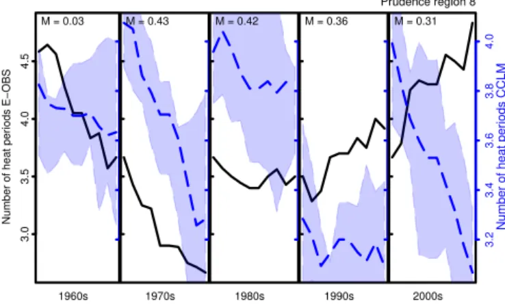
As an example, Prudence region 8 (Eastern Europe) is a region where the network method performs better than the standard approach (Figs. 5 and 6). Figure 5 shows the E-OBS number of heat periods o (black) and the CCLM ensemble mean number of heat periodsm(blue) for East-ern Europe together with the interquartile range (25th and 75th percentiles), and Fig. 6 shows again the E-OBS number of heat periods now compared to the CCLM link strength. Comparing the absolute mean differences, denoted asMin the two figures, reveals that our network approach enhances the skill in four decades, namely 1970s, 1980s, 1990s, and 2000s. Especially the 1970s, 1980s, and 1990s show a clear improvement and our network approach better reflects the low-frequency dynamics of the heat periods. The 2000s seem to be off in both model cases, the number of heat periods, and the link strength, which indicates a failed model initial-ization.
Nu m b e r o f h e a t p e ri o d s E − O B S 1960s 3.0 3.5 4.0 4.5
M = 0.03
1970s M = 0.43
1980s M = 0.42
1990s M = 0.36
2000s 3.2 3.4 3.6 3.8 4.0 Nu m b e r o f h e a t p e ri o d s C C L M
M = 0.31 Prudence region 8
Figure 5.Number of heat periods (1961–2010) in Eastern Europe (Prudence 8) in summer from E-OBSo(black) and CCLM num-ber of heat periods (blue: ensemble mean and interquartile range). The M’s denote the absolute mean difference within a decade be-tween E-OBS and the CCLM ensemble mean after normalization (see Eq. 6).
Nu m b e r o f h e a t p e ri o d s E − O B S 1960s 3.0 3.5 4.0 4.5
M = 0.14
1970s M = 0.28
1980s M = 0.36
1990s M = 0.23
2000s 0.690 0.695 0.700 0.705 0.710
Link strength CCLM
M = 0.18 Prudence region 8
Figure 6.Number of heat periods (1961–2010) in Eastern Europe (Prudence 8) in summer from E-OBS o(black) and CCLM link strength or correlation threshold W (red: ensemble mean and in-terquartile range). The M’s denote the absolute mean difference within a decade between E-OBS and the CCLM ensemble mean after normalization (see Eq. 7).
considered region, we performed the same analysis as above for the eight Prudence regions in Europe and for the 1960s, 1970s, 1980s, 1990s, and 2000s. The corresponding figures for the other regions can be found in the Supplement.
To summarize the results we calculated the absolute mean differences (Eqs. 6 and 7) for all the Prudence regions, see Fig. 7. Blue colors in the panels stand for low values (high skill) whereas red colors depict high values (low skill) in the absolute mean difference.
The left panel of Fig. 7 shows how the network method performs using only E-OBS data similar to Fig. 4. Therefore we estimated the number of heat periods in the E-OBS data and the link strength (from the complex network) of the E-OBS data and accordingly calculated the differences (after
normalization, cf. Eq. 5) between these two estimators. As can be seen blue colors dominate the plot, i.e., low differ-ences and hence high skill. Thus, this reference test shows that the link strength is coupled to the number of heat peri-ods in maximum daily summer temperature data and so can be used as an alternative, possibly better, heat period esti-mator. There are some exceptions like the 1990s and 2000s of Prudence region 6. Further investigation on the reasons of these cases has to be performed.
The middle panel of Fig. 7 shows how well the standard method performs in predicting heat periods using E-OBS ob-servations and CCLM model data. The right panel indicates the performance of the new network method in estimating heat periods using E-OBS and CCLM data. In contrast to the relatively low values in the left panel, the values in the middle and right panels on the one hand are higher for many decades and Prudence regions. On the other hand, the visual impression is that the absolute differences of the right panel are slightly smaller than those of the middle panel, especially during the 1990s and 2000s.
Thus, we can conclude with Fig. 7 that the method works in principle but that the uncertainties in the model simula-tions lead to increased differences between observasimula-tions and model simulations. In addition, the link strength seems to work better than the standard approach for the model sim-ulations with respect to the observations.
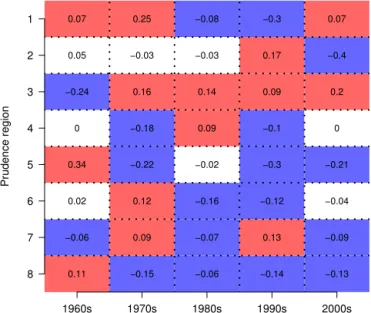
To quantify this last statement, we calculated the differ-ence between the middle and right panels of Fig. 7 (see Fig. 8). This basically shows which method performs bet-ter regarding the eight regions (columns) and five decades (rows). Blue color in Fig. 8 indicates that the network ap-proach performs better (Mdr(ψ ) < Mdr(µ)) and red color stands for a better performance of the standard approach
(Mdr(ψ ) > Mdr(µ)). White boxes in Fig. 8 denote a tie
be-tween the methods in the case of too small differences (|Mdr(ψ )−Mdr(µ)| ≤0.05). The matrix of Fig. 8 shows that the network method is clearly superior in three regions (5, 7, 8) and slightly superior in two regions (4, 6), the standard approach is superior in two regions (1, 3), and in region 2 we observed a tie, i.e., no clear result.
sam-E−OBS SD vs. sam-E−OBS link
1960s 1970s 1980s 1990s 2000s 8
7 6 5 4 3 2 1
0.25 0.1 0.31 0.18 0.46 0.22 0.08 0.06 0.31 0.26 0.2 0.13 0.17 0.51 0.54 0.07 0.01 0.31 0.3 0.1 0.19 0.23 0.2 0.27 0.37 0.15 0 0.08 0.09 0.19 0.08 0.05 0.13 0.07 0.09 0.08 0.18 0.26 0.46 0.17
E−OBS SD vs. CCLM SD
1960s 1970s 1980s 1990s 2000s 8
7 6 5 4 3 2 1
0.03 0.43 0.42 0.36 0.31 0.5 0.39 0.17 0.14 0.37 0.03 0.42 0.56 0.38 0.25 0.04 0.55 0.46 0.38 0.37 0.64 0.29 0.01 0.16 0.25 0.29 0.52 0.06 0.39 0.03 0.59 0.62 0.16 0.16 0.43 0.67 0.12 0.4 0.51 0.04
E−OBS SD vs. CCLM link
1960s 1970s 1980s 1990s 2000s 8
7 6 5 4 3 2 1
0.14 0.28 0.36 0.23 0.18 0.44 0.48 0.1 0.27 0.27 0.05 0.54 0.4 0.26 0.21 0.39 0.33 0.44 0.08 0.17 0.64 0.11 0.1 0.06 0.24 0.06 0.68 0.2 0.49 0.23 0.64 0.59 0.12 0.33 0.03 0.74 0.36 0.32 0.21 0.11
0 0.15 0.3 0.44 0.59 0.74
M v
alue
Figure 7. Absolute mean differences like in Figs. 4 to 6 of all Prudence regions for E-OBS standard approach compared to E-OBS link strength (left), to CCLM standard approach (middle), and to CCLM link strength (right).
Pr
udence region
0.07 0.25 −0.08 −0.3 0.07
0.05 −0.03 −0.03 0.17 −0.4
−0.24 0.16 0.14 0.09 0.2
0 −0.18 0.09 −0.1 0
0.34 −0.22 −0.02 −0.3 −0.21
0.02 0.12 −0.16 −0.12 −0.04
−0.06 0.09 −0.07 0.13 −0.09
0.11 −0.15 −0.06 −0.14 −0.13
1960s 1970s 1980s 1990s 2000s
8 7 6 5 4 3 2 1
Figure 8.Differences between the two right panels of Fig. 7. Blue: network approach performs better, red: standard approach performs better, white: tie.
ple sizenremains a limitation on interpretation.” and finally “propose to employ instead a simple descriptive approach for characterising the information in an ensemble. . . ”. Although we totally agree with the argumentation by von Storch and Zwiers (2013) that a “classical” significance test would most probably fail in our analysis, we think that alternative signif-icance tests, based on bootstrapping or surrogate data, could definitely help obtain a better interpretation of the results. Thus, we construct the following significance test based on surrogate data to answer the following question: what is the probability of getting a rank matrix like the one in Fig. 8 by chance?
First, we have to define what is the possibly “significant” characteristic of the matrix in Fig. 8. It is, as we concluded above, that the network method is superior in five regions. Thus the question is the following: what is the probability to
Table 2.Probability that blue matrix elements in Fig. 8 dominate in nregions by chance. Half of the elements are colored blue and red, respectively, and eight white elements are randomly added subse-quently.
Number of regionsn 1 2 3 4 5 6 7 8
Probability in % 100 99 82 35 5 0.1 0 0
observe at least five regions in which we have in each at least one blue matrix element more than a red oneby chance? Ac-cordingly we constructed matrices like in Fig. 8 by randomly coloring 20 matrix elements blue and 20 red. Afterwards we colored 8 matrix elements white as in Fig. 8. Finally, we re-peated this surrogate procedure 1000 times and counted the cases (regions) where the blue matrix elements dominate. Ta-ble 2 shows the probabilities that blue matrix elements domi-nate innregions. Since we have 16 blue elements and 16 red, it is sure that blue dominates inn=1 region, and it is impos-sible to dominate inn=7 andn=8 regions. As can be seen from Table 2 the probability of dominating inn=5 regions by chance is only about 5 %; thus the results of our network approach have to be stated significant. Due to the symmetry of the test, the same argumentation is valid for red matrix elements. Dominating inn=2 regions, as achieved by the standard approach (Fig. 8), can be realized easily by chance with a probability of approx. 99 %. Page 1 in the Supplement shows an example of 12 of these randomly generated matri-ces, where one matrix, depicted by a black frame, fulfills the “significance” criterion.
6 Conclusions and outlook
We found that the network approach is superior (signifi-cance is≈5 %) to the standard approach in estimating heat periods in Europe, hence highlighting the potential of net-work methods to improve the skill estimation in decadal pre-diction experiments. Picking up our hypothesis and simpli-fied argumentation from Sect. 3, the crucial point why we detect heat periods with the network link strength is that heat periods are cooperative events in space and time. Thus, the link strength can be used as an estimator of heat periods. The drawback of the standard approach is most probably the in-flexible threshold for the detection of heat periods (cf. Fig. 2). If the climate model contains the signal of a heat period, but with a slightly too small amplitude, the threshold will not be crossed and no heat period will be detected. In contrast, the complex climate network does not depend on such fixed thresholds and can use this information, which makes it the more robust estimator of heat periods.
The general prediction skill of climate in Europe using standard measures is still moderate. In this sense our work adds new aspects to our previous study (Mieruch et al., 2014) and also the work of Eade et al. (2012), who found a strong variation of skill with region and decade. In essence, we found regions and decades in Europe where our climate model output, or more specifically the used network estima-tor, follows the slowly evolving dynamics of observed heat periods. We also found regions and decades in which the net-work estimator is not able to represent the observational ref-erence. Understanding of this variability in prediction skill is one of the future challenges of decadal predictions.
Concluding, our approach shows that the complex climate networks approach yields meaningful climate information and has the potential to improve skill measures within the framework of climate prediction. It is the first time that such network techniques have been used in climate predictions. Since climate or decadal predictions aim to predict natural variability on the order of years, suitable statistics are needed. Natural variability on the order of years evolves highly dy-namically and often nonlinearly. Thus, the complex climate networks could bear the potential to be very useful in climate predictions. Our approach, which is even based on the most simple network measure, the node degree (or as we used it the link strength), yields optimistic results. So, we think that our analysis could be the starting point for using the com-plex networks in climate predictions. Using other measures and/or multivariate data could turn out to be the better way of analyzing predictions of natural variability years ahead than using methods from short- or medium-range forecast-ing. Further, from the network perspective it would be in-teresting to analyze other network measures like clustering, similarities, or path lengths and how they are connected to climate evolution. The incorporation of other relevant vari-ables like precipitation, wind, or soil moisture into the net-work is an appealing aspect. From a physical or climatolog-ical point of view it is important to understand why the net-work measures are able to represent climate dynamics, which
could also contribute to a better understanding of the sources of decadal predictability. Thus, the incorporation and inves-tigation of processes like the AMOC, PDO, or NAO together with complex networks and climate prediction might be an option for the future.
7 Data availability
E-OBS can be downloaded via the website www.ecad.eu.
The Supplement related to this article is available online at doi:10.5194/npg-23-307-2016-supplement.
Acknowledgements. We acknowledge the E-OBS data set from the EU-FP6 project ENSEMBLES (http://ensembles-eu.metoffice. com) and the data providers in the ECA&D project (http://www. ecad.eu).
The research programme MiKlip is funded by the German Min-istry of Education and Research (BMBF).
We also acknowledge the ETOPO1 data set (Amante and Eakins, 2009) from the NGDC (National Geophysical Data Center, Boulder, Colorado).
The article processing charges for this open-access publication were covered by a Research
Centre of the Helmholtz Association.
Edited by: A. M. Mancho
Reviewed by: four anonymous referees
References
Amante, C. and Eakins, B.: ETOPO1 1 Arc-Minute Global Relief Model: Procedures, Data Sources and Analysis. NOAA Tech-nical Memorandum, Tech. Rep. NESDIS NGDC-24, National Geophysical Data Center, NOAA, Boulder, Colorado, USA, doi:10.7289/V5C8276M, 2009.
Berezin, Y., Gozolchiani, A., Guez, O., and Havlin, S.: Sta-bility of climate networks with time, Sci. Rep., 2, 666, doi:10.1038/srep00666, 2012.
Boers, N., Bookhagen, B., Barbosa, H. M. J., Marwan, N., Kurths, J., and Marengo, J. A.: Prediction of extreme floods in the eastern Central Andes based on a complex networks approach, Nat. Commun., 5, 5199, doi:10.1038/ncomms6199, 2014. Chikamoto, Y., Timmermann, A., Luo, J.-J., Mochizuki, T.,
Ki-moto, M., Watanabe, M., Ishii, M., Xie, S.-P., and Jin, F.-F.: Skil-ful multi-year predictions of tropical trans-basin climate variabil-ity, Nat. Commun., 6, 6869, doi:10.1038/ncomms7869, 2015. Corti, S., Weisheimer, A., Palmer, T. N., Doblas-Reyes, F. J., and
Doblas-Reyes, F. J., Andreu-Burillo, I., Chikamoto, Y., García-Serrano, J., Guemas, V., Kimoto, M., Mochizuki, T., Ro-drigues, L. R. L., and van Oldenborgh, G. J.: Initialized near-term regional climate change prediction, Nat. Commun., 4, 1715, doi:10.1038/ncomms2704, 2013.
Doms, G. and Schättler, U.: A Description of the Non-Hydrostatic Regional Model LM, Part I: Dynamics and Numerics, tech. rep., Deutscher Wetterdienst, P.O. Box 100465, 63004 Offenbach, Germany, LM_F90 2.18, 2002.
Donges, J. F., Zou, Y., Marwan, N., and Kurths, J.: Complex net-works in climatic dynamics, Eur. Phys. J.-Spec. Top., 174, 157– 179, doi:10.1140/epjst/e2009-01098-2, 2009.
Donges, J. F., Donner, R. V., Trauth, M. H., Marwan, N., Schellnhuber, H.-J., and Kurths, J.: Nonlinear detection of paleoclimate-variability transitions possibly related to hu-man evolution, P. Natl. Acad. Sci. USA, 108, 20422–20427, doi:10.1073/pnas.1117052108, 2011.
Dosio, A., Panitz, H.-J., Schubert-Frisius, M., and Lüthi, D.: Dynamical downscaling of CMIP5 global circulation models over CORDEX-Africa with COSMO-CLM: evaluation over the present climate and analysis of the added value, Clim. Dynam., 44, 2637–2661, doi:10.1007/s00382-014-2262-x, 2015. Eade, R., Hamilton, E., Smith, D. M., Graham, R. J., and
Scaife, A. A.: Forecasting the number of extreme daily events out to a decade ahead, J. Geophys. Res.-Atmos., Res., 117, D21110, doi:10.1029/2012JD018015, 2012.
Frich, P., Alexander, L., Della-Marta, P., Gleason, B., Haylock, M., Klein Tank, A., and Peterson, T.: Observed coherent changes in climatic extremes during the second half of the twentieth century, Clim. Res., 19, 193–212, doi:10.3354/cr019193, 2002.
García-Serrano, J., Doblas-Reyes, F. J., Haarsma, R. J., and Polo, I.: Decadal prediction of the dominant West African mon-soon rainfall modes, J. Geophys. Res.-Atmos., 118, 5260–5279, doi:10.1002/jgrd.50465, 2013.
Giorgi, F., Jones, C., and Asrar, G.: Addressing climate information needs at the regional level: the CORDEX framework, Bull. World Meteor. Org., 58, 175–183, 2009.
Haylock, M. R., Hofstra, N., Klein Tank, A. M. G., Klok, E. J., Jones, P. D., and New, M.: A European daily high-resolution gridded data set of surface temperature and pre-cipitation for 1950–2006, J. Geophys. Res., 113, D20119, doi:10.1029/2008JD010201, 2008.
Hlinka, J., Hartman, D., Jajcay, N., Vejmelka, M., Donner, R., Mar-wan, N., Kurths, J., and Paluš, M.: Regional and inter-regional ef-fects in evolving climate networks, Nonlin. Processes Geophys., 21, 451–462, doi:10.5194/npg-21-451-2014, 2014.
Jacob, D., Petersen, J., Eggert, B., Alias, A., Christensen, O. B., Bouwer, L., Braun, A., Colette, A., Déqué, M., Georgievski, G., Georgopoulou, E., Gobiet, A., Menut, L., Nikulin, G., Haensler, A., Hempelmann, N., Jones, C., Keuler, K., Kovats, S., Kröner, N., Kotlarski, S., Kriegsmann, A., Martin, E., Meij-gaard, E., Moseley, C., Pfeifer, S., Preuschmann, S., Raderma-cher, C., Radtke, K., Rechid, D., Rounsevell, M., Samuelsson, P., Somot, S., Soussana, J.-F., Teichmann, C., Valentini, R., Vau-tard, R., Weber, B., and Yiou, P.: EURO-CORDEX: new high-resolution climate change projections for European impact re-search, Reg. Environ. Change, 14, 1–16, doi:10.1007/s10113-013-0499-2, 2013.
Kadow, C., Illing, S., Kunst, O., Rust, H. W., Pohlmann, H., Müller, W. A., and Cubasch, U.: Evaluation of forecasts by accuracy and spread in the miklip decadal climate prediction system, Meteorol. Z., doi:10.1127/metz/2015/0639, 2015.
Keenlyside, N. S., Latif, M., Jungclaus, J., Kornblueh, L., and Roeckner, E.: Advancing decadal-scale climate pre-diction in the North Atlantic sector, Nature, 453, 84–88, doi:10.1038/nature06921, 2008.
Kothe, S., Panitz, H.-J., and Ahrens, B.: Analysis of the radi-ation budget in regional climate simulradi-ations with COSMO-CLM for Africa, Meteorol. Z., 23, 123–141, doi:10.1127/0941-2948/2014/0527, 2014.
Ludescher, J., Gozolchiani, A., Bogachev, M. I., Bunde, A., Havlin, S., and Schellnhuber, H. J.: Improved El Niño forecasting by cooperativity detection, P. Natl. Acad. Sci. USA, 110, 11742– 11745, doi:10.1073/pnas.1309353110, 2013.
MacLeod, D. A., Caminade, C., and Morse, A. P.: Useful decadal climate prediction at regional scales? A look at the ENSEM-BLES stream 2 decadal hindcasts, Environ. Res. Lett., 7, 044012, doi:10.1088/1748-9326/7/4/044012, 2012.
Matei, D., Pohlmann, H., Jungclaus, J., Müller, W., Haak, H., and Marotzke, J.: Two Tales of Initializing Decadal Climate Predic-tion Experiments with the ECHAM5/MPI-OM Model, J. Cli-mate, 25, 8502–8523, doi:10.1175/JCLI-D-11-00633.1, 2012. Meehl, G. A., Teng, H., and Arblaster, J. M.: Climate model
sim-ulations of the observed early-2000s hiatus of global warming, Nature Clim. Change, 4, 898–902, doi:10.1038/nclimate2357, 2014.
Mieruch, S., Feldmann, H., Schädler, G., Lenz, C.-J., Kothe, S., and Kottmeier, C.: The regional MiKlip decadal forecast ensemble for Europe: the added value of downscaling, Geosci. Model Dev., 7, 2983–2999, doi:10.5194/gmd-7-2983-2014, 2014.
Müller, W. A., Baehr, J., Haak, H., Jungclaus, J. H., Kröger, J., Matei, D., Notz, D., Pohlmann, H., von Storch, J. S., and Marotzke, J.: Forecast skill of multi-year seasonal means in the decadal prediction system of the Max Planck In-stitute for Meteorology, Geophys. Res. Lett., 39, L22707, doi:10.1029/2012GL053326, 2012.
Peron, T. K. D., Comin, C. H., Amancio, D. R., da F. Costa, L., Rodrigues, F. A., and Kurths, J.: Correlations between climate network and relief data, Nonlin. Processes Geophys., 21, 1127– 1132, doi:10.5194/npg-21-1127-2014, 2014.
Radebach, A., Donner, R. V., Runge, J., Donges, J. F., and Kurths, J.: Disentangling different types of El Niño episodes by evolving climate network analysis, Phys. Rev. E, 88, 052807, doi:10.1103/PhysRevE.88.052807, 2013.
Scaife, A. A., Arribas, A., Blockley, E., Brookshaw, A., Clark, R. T., Dunstone, N., Eade, R., Fereday, D., Folland, C. K., Gordon, M., Hermanson, L., Knight, J. R., Lea, D. J., MacLachlan, C., Maid-ens, A., Martin, M., Peterson, A. K., Smith, D., Vellinga, M., Wallace, E., Waters, J., and Williams, A.: Skillful long-range pre-diction of European and North American winters, Geophys. Res. Lett., 41, 2514–2519, doi:10.1002/2014GL059637, 2014. Smith, D., Eade, R., and Pohlmann, H.: A comparison of full-field
and anomaly initialization for seasonal to decadal climate predic-tion, Clim. Dynam., 41, 3325–3338, doi:10.1007/s00382-013-1683-2, 2013.
Brokopf, R., Fast, I., Kinne, S., Kornblueh, L., Lohmann, U., Pincus, R., Reichler, T., and Roeckner, E.: Atmospheric compo-nent of the MPI-M Earth System Model: ECHAM6, Adv. Model. Earth Syst., 5, 146–172, doi:10.1002/jame.20015, 2013. Taylor, K. E., Stouffer, R. J., and Meehl, G. A.: An overview of
CMIP5 and the experiment design, B. Am. Meteorol. Soc., 93, 485–498, doi:10.1175/BAMS-D-11-00094.1, 2012.
Tsonis, A. A. and Swanson, K. L.: Review article “On the ori-gins of decadal climate variability: a network perspective”, Non-lin. Processes Geophys., 19, 559–568, doi:10.5194/npg-19-559-2012, 2012.
Tsonis, A. A., Swanson, K., and Kravtsov, S.: A new dynamical mechanism for major climate shifts, Geophys. Res. Lett., 34, L13705, doi:10.1029/2007GL030288, 2007.
van Oldenborgh, G. J., Doblas-Reyes, F. J., Wouters, B., and Hazeleger, W.: Skill in the trend and internal variability in a multi-model decadal prediction ensemble, Clim. Dynam., 38, 1263–1280, doi:10.1007/s00382-012-1313-4, 2012.
von Storch, H. and Zwiers, F. W.: Testing ensembles of climate change scenarios for “statistical significance”, Clim. Change, 117, 1–9, doi:10.1007/s10584-012-0551-0, 2013.