Selecting Features of Single Lead ECG Signal for Automatic Sleep Stages Classification using Correlation-based Feature Subset Selection

(1)

Selecting Features of Single Lead ECG Signal for Automatic

Sleep Stages Classification using

Correlation-based Feature Subset Selection

Ary Noviyanto1_{, Sani M. Isa}2_{, Ito Wasito}3_{and Aniati Murni Arymurthy}4

1

Computer Science, Universitas Indonesia Depok 16424/Jawa Barat, Indonesia

2

3

4

Abstract

Knowing about our sleep quality will help human life to maximize our life performance. ECG signal has potency to determine the sleep stages so that sleep quality can be measured. The data that used in this research is single lead ECG signal from the MIT-BIH Polysomnographic Database. The ECG’s features can be derived from RR interval, EDR information and raw ECG signal. Correlation-based Feature Subset Selection (CFS) is used to choose the features which are significant to determine the sleep stages. Those features will be evaluated using four different characteristic classifiers (Bayesian network, multilayer perceptron, IB1 and random forest). Performance evaluations by Bayesian network, IB1 and random forest show that CFS performs excellent. It can reduce the number of features significantly with small decreasing accuracy. The best classification result based on this research is a combination of the feature set derived from raw ECG signal and the random forest classifier.

Keywords: ECG features, Correlation-based Feature Subset Selection, RR interval, EDR, Raw ECG Signal, Sleep stages.

1. Introduction

The quality of sleep directly affects the quality of life. Using a particular measure [1], we can calculate the sleep quality of somebody by knowing the composition of his/her sleep stages. Sleep experts analyze polysomnogram data as the standard technique to determine the sleep stages. Polysomnogram is a simultaneous recording of physiological variables during sleep that include brain

activity (electroencephalogram, EEG), eye movements (electroocculogram, EOG), and chin muscle activity (electromyohram, EMG) [2].

Based on the previous works [3, 4, 5, 6], ECG as a substitute of the standard technique to determine the sleep stages has promising results. The main reason of using ECG is the expensiveness of recording process of the polysomnogram data. The data gathering has to do in a sleep laboratory that is expensive with uncomfortable processes for patients and also require trained staff. Another issue is that the sleep study (polysomnography) is costly. It means that the manual determination of the sleep stages in a long sequence of the polysomnogram data is a work that requires endurance and high accuracy. The manual determination of the sleep stages can also trigger lack standard of the sleep stages determination (i.e. every sleep expert may have different results in the sleep stages determination). The automatic processes in the polysomnography are necessary to handle the issue in the manual determination of sleep stages.

(2)

a signal from the heart during it is beating [8]. The ECG's waveform and its attributes are shown in Figure 2.

Fig. 1 Normal adult hypnogram [7].

Fig. 2 ECG’s waveforms and intervals identified [9].

Many features can be derived from only a single lead ECG signal. Several previous researches used various different features. We will define several feature sets that are constructed from single lead ECG's features and determine the best performance feature set for the automatic sleep stages classification.

2. Previous Works

Several previous researches have given promising result that ECG can be a substitute of the standard data to determine the sleep stages. Shinar et al. [3], in 2001, have used only ECG signal to detect Slow Wave Sleep (SWS) with 80% correct identification. They have used time dependent spectral component (Very Low Frequency, Low Frequency and High Frequency) that decomposed from RR interval using wavelet transform as the features.

Lewicke et al. [4], in 2008, have determined sleep and wake only using ECG signal of infants. Using fuzzy C-means (FCM) clustering algorithm, they determined that the best feature from standard Heart Rate Variability measure derived from RR interval is the mean. Using rejection approach, the model has achieved 85%-87%

correct classification while rejecting 30% of the data with a kappa statistic of 0.65-0.68.

Yilmaz et al. [5], in 2010, have investigated features that derived only from single-lead ECG to classify sleep stages and obstructive apneaic epochs. Using quadratic discriminant analysis (QDA) and support vector machines (SVM) methods have 60% or 70% accuracy for specific sleep stage on healthy subject and 89% accuracy for five obstructive sleep apnea (OSA). They have used the median, inter-quartile range, and mean absolute deviation values that derived from RR interval as the features. Bsoul et al. [6], in 2010, have done research in sleep quality assessment based on ECG measurements. They have used a multi-stage Support Vector Machines (SVM) classifier. Using a binary decision tree (BDT) technique for four classes, three-stage multi-class SVMs are needed and perform good result with high accuracy. This research uses a lot of features. For every ECG segment (i.e. 30 seconds), 112 feature measures can be extracted; 60 for RR time series and 52 for EDR time series.

3. Dataset and Features

In our research, we use ECG signal from the MIT-BIH Polysomnographic Database that can be downloaded from http://www.physionet.org [10]. The MIT-BIH Polysomnographic Database contains multiple physiologic signals during sleep. We have total 18 records of ECG signal with various recorded length from 16 subjects. From 18 records of ECG signal, we extract several features of single lead ECG signal that potentially can be used to classify the sleep stages. We have three categories of ECG's features; the features that derived from RR interval, EDR information and raw ECG signal. We can get 39 features in total with composition: 12 features from RR interval, 12 features from EDR information and 15 features from raw ECG signal. Those features will be selected and evaluated in order to determine the optimal features for the sleep stages classification.

3.1 Features Derived from RR Interval

RR interval is a distance of two successive top R waves. If the R waves are in normal beats, we can call it as NN interval (Normal to Normal interval). To describe variations of RR interval, we used Heart Rate Variability (HRV) [11]. HRV is divided into time domain measures and frequency domain measures. The common time domain measures consist of [12],

(3)

2. Standard deviation of all NN intervals (SDNN); 3. Square root of the mean of the squares of differences

between adjacent NN intervals (rMSSD);

4. Percentage of differences between adjacent NN intervals that are greater than 50 ms; a member of the larger pNNx family (pNN50);

and the common frequency domain measures consist of [12],

1. Total spectral power of all NN intervals up to 0.04 Hz (TOTPWR);

2. Total spectral power of all NN intervals between 0.003 and 0.04 Hz (VLF);

3. Total spectral power of all NN intervals between 0.04 and 0.15 Hz. (LF);

4. Total spectral power of all NN intervals between 0.15 and 0.4 Hz (HF);

5. Ratio of low to high frequency power (LF/HF). Based on Yilmaz et al. [8], we can also derived three features that belong to time domain measures; they are median, Inter-quartile range (IQR) and Mean absolute deviation (MAD). All of the features that derived from RR interval are coded using prefix “RR-” (e.g. RR-AVNN, RR-SDNN, and so on).

3.2 Features Derived from EDR

ECG signal has been related to respiratory signal [5]. Respiratory information can be derived from ECG signal, called ECG-derived respiration (EDR) information. EDR information is obtained by calculating regions under the QRS segments of ECG signal. The region is a fixed window around R point (100ms centered in R point [13]). Before we can calculate EDR from ECG signal, we have to correct ECG signal by subtracting original ECG signal with the baseline of the ECG signal. The baseline can be calculated by filtering the original ECG signal using median filter of 200 ms and 600 ms respectively [13]. From EDR information, we can also extract same features as RR interval. All of the features that derived from EDR information are coded using prefix “EDR-” (e.g. EDR-AVNN, EDR-SDNN, and so on).

3.3 Features Derived from Raw ECG Signal

Raw ECG signal is the original ECG signal without transformation into other forms (e.g. RR Interval or EDR information). They are 15 features that can be derived from raw ECG signal. The features are listed in Table 1 [14, 15].

Table 1: List of Features Derived from Raw Signal ECG [14, 15]

3.4 Dataset Construction

We construct dataset into two groups. In the first group, all of the records (18 records) are combined into a large data. In the second group, each of the record is treated as a separate data; we can call it as subject-based dataset. It is intended to find out the robustness of the classifiers and the features. Every group consists of:

1. Feature set a: it contains features that are derived from RR interval;

2. Feature set b: it contains features that are derived from EDR information;

3. Feature set c: it contains features that are derived from raw ECG signal; and

4. Feature set d: it is a combination of the features that are derived from RR interval, EDR information and from raw ECG signal.

4. Methodology

(4)

4.1 The Classifiers

A Bayesian network is a probabilistic based classifier. A Bayesian network contains a set of variables and a directed acyclic graph (DAG) as the structure that is constructed using K2 algorithm. A Bayesian network represents a probabilities distribution as Equation 1 [16] where U is a set of variable and pa(u) is parents of uϵU.

(1)

MLP (Multilayer Perceptron) is one of the neural network approaches. MLP is a generalization of single layer perceptron that consists of an input layer, one or more hidden layer and an output layer [17]. The visualization of MLP is depicted as Figure 3. The MLP uses the back-propagation learning as the learning algorithm. For this research, the number of neuron in the hidden layer is sum of the number of input neuron and the number of output neuron divided by 2.

Fig. 3 The Multilayer Perceptron.

IB1 is the simplest instance based learner that known as K -nearest neighbors with K=1. In this algorithm, the similarity measure is defined as a negative value of a Euclidean distance, according to Equation 2. How IB1 works can be described in Algorithm 1 [18].

(2) Algorithm 1: Instance Based Learning [18]

Random forest [19] is a decision tree based classifier that contains many classification trees (in this research, we generate 10 trees). The basic idea of random forest

classifier is that every single input will be classified using each classification tree in the forest and the final classification result is done by selecting the most votes in the forest.

4.2 The Feature Selection Method

The Correlation-based Feature Subset Selection (CFS) is a feature selection method based on correlation. Correlation is a degree of dependence or predictability of one variable with another [20]. Based on this technique, the feature subsets that can be signatures have two criterions: correlated with the class and uncorrelated one feature with the other. CFS calculate an evaluation measure of feature subset, called merit, using an evaluation function according to Equation 3 [20], where S is a feature subset, MS is the

heuristic merit of S, k is the feature size, rcf is the

average of feature-class correlation, and rff is the

average of feature-feature inter-correlation.

(3) To get the best feature subset, there are three possible searching techniques [20];

1. Forward selection.

This searching technique greedily adds one feature until the feature set has no higher value of the evaluation measure.

2. Backward elimination.

This searching technique greedily eliminates one by one feature until degrading value of the evaluation measure.

3. Best first.

Best first searches through the search space, either forward or backward. Because of this pure technique is exhaustive; this searching technique has a stopping criterion. The stopping criterion is no improvement value of the evaluation measure over the current best subset in five consecutive fully expanded subsets. In this research, we use the Best first with forward direction as the searching technique.

5. Experimental Results

5.1 Evaluation Measures

(5)

convince about the results of evaluation measures, we use k-fold validation method with k = 10.

Table 2: Interpretation of Kappa Statistic [21]

Kappa Agreement

< 0 Less than chance agreement

0.01 - 0.20 Slight agreement

0.21 - 0.40 Fair agreement

0.41 - 0.60 Moderate agreement

0.61 - 0.80 Substantial agreement

0.81 - 0.99 Almost perfect agreement

5.2 Feature Selection Results

Using CFS, we can take the best selected features for the feature set that derived from RR interval, EDR information and Raw ECG signal.

1. Features derived from RR interval.

From 12 features in total, there are 6 selected features; RR-rMSSD, RR-pNN50, RR-TOTPWR, RR-VLF, RR-LF/HF and RR-MAD.

2. Features derived from EDR information.

From 12 features in total, there are 5 selected features; EDR-TOTPWR, EDR-VLF, EDR-LF, EDR-HF and EDR-LF/HF.

3. Features derived from Raw ECG signal.

From 15 features in total, there are 5 selected features; 4th Power, Katz Fractal Dim, Hjorth Mobility, Hjorth Complexity and PFD.

4. Features derived from RR interval, EDR information and Raw ECG signal.

From 39 features in total, there are 14 selected features; rMSSD, TOTPWR, LF/HF, RR-MAD, EDR-VLF, EDR-LF, EDR-HF, EDR-LF/HF, 4th Power, Katz Fractal Dim, HFD, Hjorth Mobility, Hjorth Complexity and PFD.

Based on these results, the features that are selected in the features selection process of the feature set d (i.e. combination of RR interval, EDR information and Raw ECG signal) are also selected in the features selection process of the feature set a (i.e. RR interval), b (i.e. EDR information) or c (i.e. Raw ECG signal) but not vice versa. For example, RR-rMSSD is selected in the features selection process of the feature set d and also selected in the features selection of the feature set a; RR-pNN50 is selected in the features selection process of the feature set a but not selected in features selection process of the feature set d.

5.2 Result and Discussion

The classification results of the first group dataset are presented in Table 3 and Table 4. We can depict them into line chart in Figure 4. Based on Figure 4, the graphic of dash line and continues line in Bayesian network, IB1 and random forest have shape same pattern. We can see in Figure 4b; multilayer perceptron does not have same shape pattern. Reducing features in the feature set c with MLP as the classifier has decreased the accuracy for 10.65%.

Table 3: The classification result using the full set features; %C is percent correct classification and K is the Kappa statistic

Feature Set

BN MLP IB1 RF

%C K %C K %C K %C K

a 41.01 0.24 48.87 0.23 40.00 0.17 50.33 0.28 b 42.69 0.26 54.10 0.30 48.35 0.29 55.73 0.36 c 59.01 0.45 59.32 0.41 79.34 0.71 79.80 0.72 d 60.53 0.48 68.12 0.55 70.56 0.59 76.24 0.66

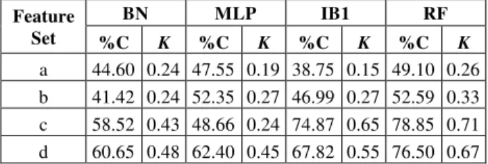
Table 4: The classification result using the best selected features; %C is percent correct classification and K is the Kappa statistic Feature

Set

%C K %C K %C K %C K

a 44.60 0.24 47.55 0.19 38.75 0.15 49.10 0.26 b 41.42 0.24 52.35 0.27 46.99 0.27 52.59 0.33 c 58.52 0.43 48.66 0.24 74.87 0.65 78.85 0.71 d 60.65 0.48 62.40 0.45 67.82 0.55 76.50 0.67

Table 5: Comparison of decreasing accuracy and number of features; DA is Decreasing of Accuracy in percent and DN is Decreasing of Number

of Features in percent.

Feature set

DA DN DA DN DA DN DA DN

a -3.59 50.00 1.32 50.00 1.25 50.00 1.22 50.00 b 1.27 58.33 1.75 58.33 1.36 58.33 3.14 58.33 c 0.49 66.67 10.65 66.67 4.47 66.67 0.95 66.67 d -0.13 64.10 5.72 64.10 2.74 64.10 -0.26 64.10

(6)

Fig. 4 The effect of feature selection in accuracy over the classifiers; y-axis is correctly classified in percent and x-y-axis is the feature set; dash line is using selected features and continues line is using full set features.

Fig. 5 Comparison of the feature sets; a, b, c, and d are the feature set; y-axis is correctly classified in percent and x-y-axis is the classifiers.

The line chart in Figure 5 that derived from Table 3 and Table 4 shows the performance of the feature sets. Overall,

feature set c and d are better than feature set a and feature set b for all classifiers. Based on this experiment, the feature set c and feature set d which include raw ECG signal show good performance to determine the sleep stages for the all classifiers.

According to the result in Table 3 and Table 4, the best performance of Bayesian network and Multilayer perceptron are achieved when using the feature set d (i.e. combination of features that derived from RR interval, EDR information and raw ECG signal) in both cases; with and without features selection. Whereas the best performance of IB1 and Random forest are achieved when using the feature set c (i.e. the features that derived from raw signal ECG) in both cases.

In the experiment using combination all of records (i.e. first group dataset); the best accuracy is 79.80% with 0.72 kappa statistic. This performance is achieved using the random forest as the classifier and 15 features that derived from raw ECG signal (i.e. the feature set c without feature selection). Using CFS, the best accuracy is 78.85% with 0.71 kappa statistic. This performance is achieved using the random forest as the classifier and 5 selected features that derived from raw ECG signal. CFS can reduce 66.67% number of features in the feature set c, from 15 features becomes 5 features. The accuracy is reduced by 0.95% and the kappa statistic is reduced by 0.01.

The comparison results of subject based dataset (i.e. second group dataset) are show in Table 6, 8, 10, and 12 for full set features and Table 7, 9, 11, and 13 for selected features. To simplify our analysis we can resume Table 6, 8, 10, and 12 into Table 14 and Table 7, 9, 11, and 13 into Table 15. Using subject based dataset, the random forest classifier and the feature set c that derived from raw ECG signal do the best performance with overall average percent correct classification is 80.95% and the average of kappa statistic is 0.70 in full set features. The random forest classifier and the feature set c do the best performance also in the selected features using CFS; overall average percent correct classification is 79.78% and the average kappa statistic is 0.68. CFS can decrease 66.67% number of features, from 15 features becomes 5 features with only 1.17% decreasing of average percent correct classification and 0,02 decreasing of average kappa statistic. This best result is close to IB1. IB1 using the feature set c can achieve 80.54% average percent correct classification and 0.70 average kappa statistics in full set features; 79.29% average percent correct classification and 0.68 average kappa statistics in selected features.

Table 6: Percent correct comparison of every records using feature set a

(7)

Rec. BN MLP IB1 RF

%C K %C K %C K %C K

slp01a 60.40 0.42 58.10 0.38 55.21 0.35 61.09 0.42 slp01b 56.31 0.25 60.18 0.31 59.39 0.33 63.93 0.37 slp02a 64.02 0.46 77.18 0.60 73.73 0.56 76.60 0.58 slp02b 72.30 0.57 77.80 0.64 76.04 0.62 77.26 0.63 slp03 44.99 0.29 54.96 0.33 45.38 0.24 57.37 0.37 slp04 58.32 0.36 66.48 0.32 64.12 0.36 69.48 0.40 slp14 45.06 0.23 52.74 0.28 45.97 0.23 53.94 0.30 slp16 62.58 0.46 64.90 0.47 58.26 0.39 66.33 0.49 slp32 72.23 0.52 77.27 0.57 72.78 0.51 78.21 0.58 slp37 77.33 0.37 89.59 0.55 84.50 0.41 89.08 0.51 slp41 43.23 0.23 49.15 0.30 45.66 0.26 52.10 0.34 slp45 52.14 0.18 58.18 0.15 53.83 0.21 61.22 0.18 slp48 51.96 0.32 57.95 0.38 53.79 0.33 58.70 0.40 slp59 54.20 0.42 56.34 0.44 50.08 0.36 57.92 0.45 slp60 71.15 0.51 71.06 0.49 58.95 0.33 74.52 0.55 slp61 47.33 0.29 54.74 0.33 46.27 0.25 54.00 0.33 slp66 65.61 0.48 67.00 0.50 58.71 0.38 67.32 0.50 slp67x 51.77 0.25 55.04 0.30 55.64 0.32 61.08 0.38

Avg. 58.39 0.37 63.81 0.41 58.80 0.36 65.56 0.43

Table 7: Percent correct comparison of every records using feature set a

with feature selection; %C is percent correct classification and K is the Kappa statistic

%C K %C K %C K %C K

Avg. 60.35 0.37 64.71 0.41 58.84 0.36 65.30 0.43

Table 8: Percent correct comparison of every records using feature set b

without feature selection; %C is percent correct classification and K is the Kappa statistic

%C K %C K %C K %C K

Avg. 58.87 0.39 64.88 0.42 61.32 0.39 66.59 0.45

Table 9: Percent correct comparison of every records using feature set b

%C K %C K %C K %C K

(8)

Table 10: Percent correct comparison of every records using feature set c

%C K %C K %C K %C K

Avg. 68.68 0.53 79.29 0.67 80.54 0.70 80.95 0.70

Table 11: Percent correct comparison of every records using feature set c

%C K %C K %C K %C K

Avg. 72.16 0.56 74.84 0.59 79.29 0.68 79.78 0.68

Table 12: Percent correct comparison of every records using feature set d

%C K %C K %C K %C K

Avg. 69.36 0.55 76.42 0.63 76.41 0.63 80.00 0.68

Table 13: Percent correct comparison of every records using feature set d

%C K %C K %C K %C K

(9)

Table 14: Average percent correct comparison of every feature set without feature selection; %C is percent correct classification and K is

the Kappa statistic

Feature set

%C K %C K %C K %C K

a 58.39 0.37 63.81 0.41 58.80 0.36 65.56 0.43 b 58.87 0.39 64.88 0.42 61.32 0.39 66.59 0.45 c 68.68 0.53 79.29 0.67 80.54 0.70 80.95 0.70 d 69.36 0.55 76.42 0.63 76.41 0.63 80.00 0.68

Table 15: Average percent correct comparison of every feature set with feature selection; %C is percent correct classification and K is the Kappa

statistic

Feature set

%C K %C K %C K %C K

a 60.35 0.37 64.71 0.41 58.84 0.36 65.30 0.43 b 60.17 0.38 64.66 0.39 62.98 0.42 66.96 0.47 c 72.16 0.56 74.84 0.59 79.29 0.68 79.78 0.68 d 71.14 0.56 76.43 0.63 76.33 0.63 79.50 0.67

4. Conclusions

The CFS shows good result for Bayesian network, IB1 and random forest with relatively small amount in decreasing accuracy and significantly reducing the number of the features but it is not too good for multilayer perceptron. Increasing accuracy in Table 5 indicates that not all features will be useful and adding inappropriate features may decrease the accuracy of some classifiers. For example Bayesian network classifier with selected feature set a and feature set d, random forest classifier with selected feature set d. Multilayer perceptron and IB1 always show better results when not reducing the number of features using the features selection method.

Overall, random forest classifier is better than Bayesian network, multilayer perceptron or IB1 for any feature sets in the first group dataset. On the other hand, based on our experiment and setting, the features that derived from raw ECG signal have more potency to be the signature of sleep stages than the features that derived from RR interval or EDR information. This feature set has higher accuracy and kappa statistic than the others. The combination of the random forest classifier and the features that derived from raw ECG signal shows the best performance. Using full set features from raw ECG signal, we can get 79.80% correctly classified instances and 0.72 kappa statistic. CFS as feature selection method shows good result. We can reduce 66.67% number of features that derived from raw ECG signal and only reduce 0.95% accuracy and 0.01 kappa statistic. The accuracy becomes 78.85% and the kappa statistic becomes 0.71.

The experiments using subject based dataset support our conclusion that the combination of the random forest as the classifier and the features that derived from raw ECG signal perform better result than the others. Using full set features from raw ECG signal, we can get 80.95% of average percent correct classification and 0.70 average kappa statistic. CFS also performs well; using selected features, we can get 79.78% average percent correct classification and 0.68 average kappa statistics; it means only reduce 1.17% in the average percent correct classification and 0.02 in the average kappa statistics. This results show almost the same with the first group dataset. It means the classifiers and the feature set are robust.

Acknowledgments

This research as a part of research grant with title Development Of Sleep-Awakening Timing Controller for Occupational Safety and Health Based-On Computational Intelligent Algorithm was supported by Universitas Indonesia.

References

[1] American Academy of Sleep Medicine, International classification of sleep disorders, revised: Diagnostic and coding manual, Chicago, Illinois: American Academy of Sleep Medicine, 2001.

[2] C. Pollak, M.J. Thorpy, and J. Yager. The Encyclopedia of Sleep and Sleep Disorders. Facts on File library of health and living. New York: Facts on File, 2009.

[3] Z. Shinar et al., “Automatic detection of slow-wave-sleep using heart rate variability”, Computers in Cardiology 2001, 2001, pp. 593-596.

[4] A. Lewicke, et al., “Sleep versus wake classification from heart rate variability using computational intelligence: consideration of rejection in classification models”, IEEE Trans Biomed Eng, Vol. 55, No. 1, 2008, pp. 108–18. [5] B. Yilmaz et al., “Sleep stage and obstructive apneaic

epoch classification using single-lead ecg”, BioMedical Engineering OnLine, Vol. 9, No. 1, 2010, pp. 39.

[6] M. Bsoul et al., “Real-time sleep quality assessment using single-lead ECG and multi-stage SVM classifier”, in the International Conference of IEEE Engineering in Medicine and Biology Society, 2010, Vol 2010, pp 1178–1181. [7] J.M. Shneerson. Sleep medicine: a guide to sleep and its

disorders, Oxford: Blackwell Publishing, 2005.

[8] G. D. Clifford, F. Azuaje, and P. McSharry, Advanced Methods And Tools for ECG Data Analysis, USA:Artech House, Inc., 2006.

[9] R. V. Andreo, B. Dorizzi, and J. Boudy, “Ecg signal analysis through hidden markov models”, IEEE Transactions on Biomedical Engineering, Vol. 53, No. 8, 2006, pp. 1541–1549.

(10)

[11]“Heart rate variability: standards of measurement, physiological interpretation and clinical use. Task Force of the European Society of Cardiology and the North American Society of Pacing and lectrophysiology”,

Circulation, Vol. 93, No. 5, 1996, pp. 1043–1065.

[12]J. E. Mietus. Time domain measures:from variance to pnnx. Internet: http://physionet.org/events/hrv-2006/mietus-1.pdf. June 2011.

[13]P. de Chazal, T. Penzel, and C. Heneghan, “Automated detection of obstructive sleep apnoea at different time scales using the electrocardiogram”, Physiological Measurement, Vol. 25, No. 4, 2004, pp. 967.

[14]F. S. Bao, X. Liu, and C. Zhang, “PyEEG:An open source python module for EEG/MEG feature extraction. Comp. Int. and Neurosc., Vol. 2011, 2011.

[15]M. Wiggins et al., Evolving a bayesian classifier for ecg-based age classification in medical applications. Applied Soft Computing, Vol. 8, No. 1, 2008, pp. 599 – 608. [16]R. R. Bouckaert, “Bayesian network classifiers in weka”,

Technical report, University of Waikato, May 2008. [17]S. Haykin, Neural Networks: A Comprehensive Foundation

(2nd edition), Upper Saddle River, NJ: Prentice Hall, 1999. [18]D. W. Aha and D. Kibler. “Instance-based learning

algorithms”, In Machine Learning, 1991, pp 37–66. [19]L. Breiman, “Random forests”, Mach. Learn., Vol. 45, 2001,

pp. 5–32.

[20]M. A. Hall, “Correlation-based Feature Subset Selection for Machine Learning”, PhD thesis, University of Waikato, Hamilton, New Zealand, 1998.

[21]A. J. Viera and J. M. Garrett, “Understanding Interobserver Agreement: The Kappa Statistic”, Family Medicine, Vol. 37, No. 5, 2005, pp. 360–363.

Ary Noviyanto holds Bachelor degree in Computer Science from

Department of Computer Science, Universitas Gadjah Mada, Indonesia. He is a research assistant for image processing and pattern recognition laboratory in faculty of computer science, Universitas Indonesia.

Sani M. Isa holds Bachelor degree in Mathematics from Faculty of

Natural Science, Padjadjaran University, Indonesia; and Master degree from Faculty of Computer Science, University of Indonesia.

Ito Wasito holds Ph.D in Computer Science, School of Computer

Science and Information Systems, Birkbeck College, University of London, United Kingdom.

Aniati Murni Arymurthy holds Bachelor degree in Electrical