An automated method to build groundwater model hydrostratigraphy from airborne electromagnetic data and lithological borehole logs

(1)

HESSD

12, 1555–1598, 2015

An automated method to build groundwater model

hydrostratigraphy

P. A. Marker et al.

Title Page

Abstract Introduction

Conclusions References

Tables Figures

◭ ◮

Back Close

Full Screen / Esc

Printer-friendly Version Interactive Discussion

Discussion

P

a

per

|

Discussion

P

a

per

|

Discussion

P

a

per

|

Discussion

P

a

per

|

Hydrol. Earth Syst. Sci. Discuss., 12, 1555–1598, 2015 www.hydrol-earth-syst-sci-discuss.net/12/1555/2015/ doi:10.5194/hessd-12-1555-2015

This discussion paper is/has been under review for the journal Hydrology and Earth System Sciences (HESS). Please refer to the corresponding final paper in HESS if available.

An automated method to build

groundwater model hydrostratigraphy

from airborne electromagnetic data and

lithological borehole logs

P. A. Marker1, N. Foged2, X. He3, A. V. Christiansen2, J. C. Refsgaard3, E. Auken2, and P. Bauer-Gottwein1

1

Department of Environmental Engineering, Technical University of Denmark, Kgs. Lyngby, Denmark

2

HydroGeophysics Group, Department of Geoscience, Aarhus University, Aarhus, Denmark

3

Geological Survey of Denmark and Greenland, Copenhagen, Denmark

Received: 22 December 2014 – Accepted: 11 January 2015 – Published: 2 February 2015

Correspondence to: P. A. Marker (paam@env.dtu.dk)

(2)

HESSD

12, 1555–1598, 2015

P. A. Marker et al.

Title Page

Tables Figures

◭ ◮

Back Close

Full Screen / Esc

Discussion

P

a

per

|

Discussion

P

a

per

|

Discussion

P

a

per

|

Discussion

P

a

per

|

Abstract

Large-scale integrated hydrological models are important decision support tools in wa-ter resources management. The largest source of uncertainty in such models is the hy-drostratigraphic model. Geometry and configuration of hydrogeological units are often poorly determined from hydrogeological data alone. Due to sparse sampling in space,

5

lithological borehole logs may overlook structures that are important for groundwater flow at larger scales. Good spatial coverage along with high spatial resolution makes airborne time-domain electromagnetic (AEM) data valuable for the structural input to large-scale groundwater models. We present a novel method to automatically integrate large AEM data-sets and lithological information into large-scale hydrological models.

10

Clay-fraction maps are produced by translating geophysical resistivity into clay-fraction values using lithological borehole information. Voxel models of electrical resistivity and clay fraction are classified into hydrostratigraphic zones usingk-means clustering. Hy-draulic conductivity values of the zones are estimated by hydrological calibration using hydraulic head and stream discharge observations. The method is applied to a

Dan-15

ish case study. Benchmarking hydrological performance by comparison of simulated hydrological state variables, the cluster model performed competitively. Calibrations of 11 hydrostratigraphic cluster models with 1–11 hydraulic conductivity zones showed improved hydrological performance with increasing number of clusters. Beyond the 5-cluster model hydrological performance did not improve. Due to reproducibility and

pos-20

(3)

HESSD

12, 1555–1598, 2015

P. A. Marker et al.

Title Page

Tables Figures

◭ ◮

Back Close

Full Screen / Esc

Discussion

P

a

per

|

Discussion

P

a

per

|

Discussion

P

a

per

|

Discussion

P

a

per

|

1 Introduction

Large-scale distributed integrated hydrological and groundwater models are used ex-tensively for water resources management and research. We use large-scale to refer to models in the scale of 100 to 1000 km2 or larger. Examples are: water resources management in water scares regions (Gräbe et al., 2012; Laronne Ben-Itzhak and

5

Gvirtzman, 2005); groundwater depletion (Scanlon et al., 2012); contamination (Li and Merchant, 2013; Mukherjee et al., 2007); agricultural impacts on hydrogeological sys-tems (Rossman and Zlotnik, 2013); and well capture zone delineation (Moutsopoulos et al., 2007; Selle et al., 2013).

Such models are typically distributed, highly parameterized, and depend on data

10

availability to suffi_{ciently represent the modelled systems. Model parameterization} in-cludes, for example, the saturated and unsaturated zone hydraulic properties, land use distribution and properties, and stream bed configuration and properties. Hydrologi-cal forcing data such as precipitation and temperature are also required. Parameters are estimated through calibration, which requires hydrological observation data

com-15

monly in the form of groundwater hydraulic heads and stream discharges. Calibration data should be temporally and spatially representative for the modelled system, and so should validation data sets.

One of the main challenges in modelling large-scale hydrogeological systems is data scarcity (Refsgaard et al., 2010; Zhou et al., 2014). Uncertainty inherent in distributed

20

hydrological models is well known (Beven, 1989). Incorrect system representation due to lack of data contributes to this uncertainty, but most important source of uncertainty in distributed groundwater models is incorrect representation of geologic structures (Refsgaard et al., 2012; Seifert et al., 2012; Zhou et al., 2014).

Lithological borehole logs are the fundamental data source for constructing

hydros-25

(4)

HESSD

12, 1555–1598, 2015

P. A. Marker et al.

Title Page

Tables Figures

◭ ◮

Back Close

Full Screen / Esc

Discussion

P

a

per

|

Discussion

P

a

per

|

Discussion

P

a

per

|

Discussion

P

a

per

|

geological domain and hence the model area often needs to be subdivided into several stationary geological domains. Spatial inconsistent sampling pattern and scarcity make lithological borehole logs alone insuffi_{cient to capture local-scale geological structures} relevant for simulation of groundwater flow and contaminant transport.

Airborne time-domain electromagnetic (AEM) data is unique with respect to good

5

spatial coverage and high resolution. AEM is the only technique that can provide high-resolution subsurface information at regional scales. Geological structures and hetero-geneity, which spatially scarce borehole lithology data may overlook, are well resolved in AEM data. Geophysical data and especially AEM data are commonly used to sup-port lithological borehole information in geological mapping and modelling (Bosch et al.,

10

2009; Høyer et al., 2011; Jorgensen et al., 2010; Jørgensen et al., 2013; Sandersen and Jorgensen, 2003).

Current practice for hydrostratigraphic and geological model generation faces a num-ber of challenges: structures that control groundwater flow may be overlooked in the manual 3-D modelling process; geological models are subjective, and different

geolog-15

ical models may result in very diff_{erent hydrological predictions; structural uncertainty} inherent in the model building process cannot be quantified. Currently there is no stan-dardized way of integrating high resolution AEM into hydrogeological models.

Sequential, joint and coupled hydrogeophysical inversion methods have been de-veloped and used extensively in hydrological and groundwater research to capture

20

hydrological processes or estimate aquifer properties and structures from geophys-ical data (Hinnell et al., 2010). Hydrogeophysgeophys-ical inversion addresses hydrogeologi-cal property estimation or delineation of hydrogeologihydrogeologi-cal structures. In the context of large-scale groundwater models studies, Dam and Christensen (2003) and Hercken-rath et al. (2013) translate between hydraulic conductivity and electrical resistivity to

25

(5)

hy-HESSD

12, 1555–1598, 2015

P. A. Marker et al.

Title Page

Tables Figures

◭ ◮

Back Close

Full Screen / Esc

Discussion

P

a

per

|

Discussion

P

a

per

|

Discussion

P

a

per

|

Discussion

P

a

per

|

drogeophysical inversion was preferred over joint hydrogeophysical inversion due to the uncertainty associated with the translator function. Structural inversions are often performed as purely geophysical inversions, where subsurface structures (that mimic geological or hydrogeological features) are favoured during inversion by choosing ap-propriate regularization terms. An example is the layered and laterally constrained

in-5

version developed by Auken and Christiansen (2004), which respects vertically sharp and laterally smooth boundaries found in sedimentary geology. Joint geophysical inver-sions have been used extensively to delineate subsurface hydrogeological structures under the assumption that multiple geophysical data sets carry information about the same structural features of the subsurface (Christiansen et al., 2007; Gallardo, 2003;

10

Haber and Oldenburg, 1997) but examples of successful joint hydrogeophysical inver-sion at larger scales are rare.

As a response to lack of global petro-physical relationships, clustering algorithms as an extension to structural inversion methods have been applied in geophysics (Bedrosian et al., 2007). Fuzzy c-means and k-means clustering algorithms have

15

been used with sequential inversion schemes (Paasche et al., 2006; Triantafilis and Buchanan, 2009) and joint inversion schemes (Di Giuseppe et al., 2014; Paasche and Tronicke, 2007). These studies have focused on the structural information contained in geophysical information, and hydrogeological or geological parameters of the sub-surface are assumed uniform within the delineated zones. This approach corresponds

20

well with the common practice in groundwater modelling where degrees of freedom of the subsurface are reduced by zoning the subsurface.

We present an objective and semi-automatic method to model large-scale hydros-tratigraphy from geophysical resistivity and lithological data. The method is a novel sequential hydrogeophysical inversion for integration of AEM data into the

hydrolog-25

(6)

HESSD

12, 1555–1598, 2015

P. A. Marker et al.

Title Page

Tables Figures

◭ ◮

Back Close

Full Screen / Esc

Discussion

P

a

per

|

Discussion

P

a

per

|

Discussion

P

a

per

|

Discussion

P

a

per

|

assumed to have uniform hydrogeological properties, and thus form the hydrostrati-graphic model. Third, the hydraulic conductivity (K) of each zone in the hydrostrati-graphic cluster model is estimated in a hydrological model calibration. The hydrological performance is benchmarked against a geological reference model. Results are shown for a Danish case study.

5

2 Materials and methods

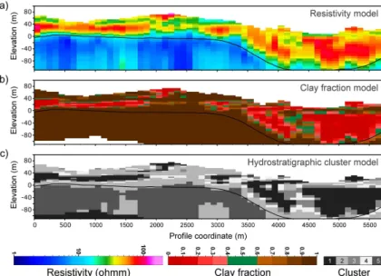
We propose a data-driven 3-D zonation method to build groundwater model hydros-tratigraphy. Hydrostratigraphic structures and parameters are determined sequentially by geophysical/lithological and hydrological data respectively. As shown in Fig. 1 zona-tion is completed in two steps, (1) delineazona-tion of hydrostratigraphic structures (see

10

Fig. 2c) through k-means cluster analysis on resistivity data (see Fig. 2a) and clay fraction values (see Fig. 2b), and (2) estimation of hydraulic parameters of the hydros-tratigraphic structures in a hydrological calibration using observations of hydraulic head and stream discharge.

11 hydrostratigraphic cluster models consisting of 1–11 zones are set up and

cali-15

brated.

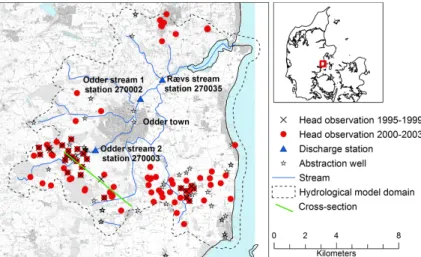
2.1 Study area

Norsminde study area is located on the eastern coast of Jutland, Denmark, and covers a land surface area of 154 km2. Figure 3 shows a map of the area delineating study area boundary, streams, and hydrological data. An overview of the geophysical and

20

lithological data is shown in Fig. 4. Within 5–7 km from the sea, the land is flat and rises only to 5–10 m a.s.l. Further to the west the land ascends into an up-folded end-moraine at elevations between 50–100 m a.s.l. The town of Odder with approximately 20 000 inhabitants is located at the edge of the flat terrain in the middle of the model domain.

(7)

HESSD

12, 1555–1598, 2015

P. A. Marker et al.

Title Page

Tables Figures

◭ ◮

Back Close

Full Screen / Esc

Discussion

P

a

per

|

Discussion

P

a

per

|

Discussion

P

a

per

|

Discussion

P

a

per

|

Palaeogene, Neogene and Quaternary deposits characterize the area. The Palaeo-gene deposits are thick clays, and define the lower geological boundary. NeoPalaeo-gene marine clays interbedded with alluvial sands overlay the Palaeogene deposits in the elevated northern and western parts of the model domain. Quaternary deposits are glacial meltwater sediments and tills found throughout the domain. A large WE striking

5

tunnel valley (2 km by 14 km) incises the Palaeogene clay in the south (Jørgensen and Sandersen, 2006). The unconsolidated fill materials are meltwater sand and gravel, clay tills, and waterlaid silt/clay.

Groundwater is abstracted for drinking water supply, mainly from tunnel valley deposits and the elevated south-western part of the domain. The groundwater

re-10

source is abstracted from 66 abstraction wells, with a total production of 18 000– 26 000 m3yr−1_{, excluding smaller private wells. Maximum annual abstraction from one} well is 12 400 m3yr−1_{. Actual pumping variation among the 66 wells and inter-annual} variation of pumping rates are unknown. Abstraction is planned locally by water works and only information about permissible annual rates has been obtained for this study.

15

Groundwater hydraulic heads are available from 132 wells at various depths, see Fig. 3 for the spatial distribution. Hydraulic head data are collected from the Danish national geological and hydrological database Jupiter (GEUS, n.d.).

Average annual precipitation is 840 mm yr−1 _{for the years 1990–2011. Most of the} area is tile-drained. The catchment is drained by a network of 24 streams; the main

20

stream is gauged at the three stations 270035, 270002 and 270003 (see Fig. 3). Streams vary from ditch-like channels to meters wide streams. Low and high flows respectively are in the order of 0.05–0.5 and 0.5–5 m3s−1_{. Daily stream discharge data} is available from three gauging stations. Discharges are calculated from mean daily water table measurements and translated with QH curves, which are available from

25

(8)

HESSD

12, 1555–1598, 2015

P. A. Marker et al.

Title Page

Tables Figures

◭ ◮

Back Close

Full Screen / Esc

Discussion

P

a

per

|

Discussion

P

a

per

|

Discussion

P

a

per

|

Discussion

P

a

per

|

2.2 Geophysical data

Time-domain electro-magnetic (AEM) data collected through ground and airborne sur-veys is available for most of the study area; brown dashed areas in Fig. 4a show the extent of the ground-based surveys and dots in Fig. 4a show locations of AEM sound-ings. AEM data was collected using the SkyTEM101 system in 2011 (Schamper et al.,

5

2014a). SkyTEM101 is developed for near-surface exploration by measuring also very early time gates, which requires careful system calibration and data processing (Auken et al., 2009; Schamper et al., 2014a). Depth of investigation (DOI) (Auken et al., 2014; Christiansen and Auken, 2012) varied between 50 and 150 m. The survey was com-pleted with a flight line spacing of 100/50 m and sounding spacing of 15 m (total of

10

1856 line km, equivalent to 106 770 1-D resistivity models). Data was inverted using spatially constrained inversion (SCI), which mimics 3-D distribution of subsurface resis-tivity by passing information through lateral and vertical constraints along and between flight lines (Viezzoli et al., 2008). In the SCI, single soundings were modelled as smooth 1-D resistivity models consisting of 29 layers with fixed layer boundaries. DOI was used

15

to terminate the resistivity models with depth. For the airborne survey an acceptable match of almost 90 % was found when checking resistivity results against borehole data (Schamper et al., 2014b). Ground based TEM soundings were collected during the 1990’s with the Geonics TEM47/PROTEM system, and were inverted individually as 1-D layered resistivity models. Depending on optimal fit these models have 3–5

20

layers.

2.3 Hydrostratigraphic model

Geophysical and lithological data are used to zone the subsurface. Geophysical data consists of resistivity values determined from inversion of airborne and ground-based electromagnetic data. Lithological information is represented in clay fraction values

25

(9)

HESSD

12, 1555–1598, 2015

P. A. Marker et al.

Title Page

Tables Figures

◭ ◮

Back Close

Full Screen / Esc

Discussion

P

a

per

|

Discussion

P

a

per

|

Discussion

P

a

per

|

Discussion

P

a

per

|

The CF-concept is formulated as a least squares inversion problem to determine the parameters of a petro-physical relationship that translates geophysical resistivities into clay fraction values. The concept is described in detail in Foged et al. (2014) and (Christiansen et al., 2014), and only a brief introduction is given here. The inversion minimizes the diff_{erence between observed clay fraction as determined from borehole}

5

lithological logs (in the inversion this is the data) and translated clay fraction as deter-mined from geophysical resistivity values (in the inversion this is the forward data). Clay fraction expresses relative accumulated thickness of clay material over an interval. In this context clay refers to material described as clay in lithological logs, and not clay minerals. Clay definitions include, among others, clay till, marl clay, mica clay, and silty

10

clay. Lithological borehole information is available at approximately 700 locations (see Fig. 4b). Descriptions are from the Danish Jupiter database (GEUS, n.d.) and level of detail and quality varies from detailed lithological description at 1 m intervals to more simple sand, clay, till descriptions at layer interface depths. Boreholes are categorized according to quality of lithological information where 1 is the highest quality and 5 is

15

the lowest (see Fig. 4b). The quality rating is presented in Schamper et al. (2014b). In the CF-inversion, the petrophysical relationship (in the inversion this is the forward model) is a two-parameter function defined in regular horizontal 2-D grids which are vertically constrained to form a 3-D model. The translator model parameters are inter-polated from grid nodes to the locations of the geophysical resistivity models. Using the

20

location-specific model, geophysical resistivities are translated into clay fraction values. Using kriging the simulated clay fractions are interpolated to the location of the litholog-ical borehole logs. The misfit between the observed and simulated clay fractions are then calculated at the borehole locations. The objective function, which contains data misfit and vertical and horizontal smoothness constraints, is optimized iteratively.

25

(10)

HESSD

12, 1555–1598, 2015

P. A. Marker et al.

Title Page

Tables Figures

◭ ◮

Back Close

Full Screen / Esc

Discussion

P

a

per

|

Discussion

P

a

per

|

Discussion

P

a

per

|

Discussion

P

a

per

|

example till and Palaeogene clay have respectively medium and low resistivity values while the clay fraction for both materials is 1.

K-means clustering is a well-known cluster analysis which finds groups in multivari-ate data based on a measure of similarity between cluster members (Wu, 2012). Simi-larity is defined as minimum squared Euclidean distance between each cluster member

5

and cluster centroid, summed over all cluster members. The number of clusters that data is divided into is defined by the user. We use the k-means analysis implemen-tation in MATLAB R2013a, which use a two-phase search, batch and sequential, to minimize the risk of reaching a local minimum.

Because clay fraction values are correlated with geophysical resistivities k-means

10

clustering is performed on principal components (PC) of the original variables. Principal components analysis (PCA) is an orthogonal transformation based on data variances (Hotelling, 1933). PCA thus finds uncorrelated linear combinations of original data while obtaining maximum variance of the linear combinations (Härdle and Simar, 2012). The uncorrelated PCs are a useful representation of the original variables as input to ak

-15

means cluster analysis. Original variables must be weighted and scaled prior to PCA, as PCA is scale sensitive, and the lack of explicit physical meaning of the PCs makes weighting diffi_{cult. Clay fraction values are unchanged as they range between 0 and 1.} The normalized resistivity values are calculated asρ_norm= logρ−logρmin

logρ_max−logρmin. Where ρmin is andρ_maxis minimum and maximum resistivity values respectively.

20

2.4 Integrated hydrological model

Hydrological data are used to parameterise the structures of the hydrostratigraphic model. Stream discharges and groundwater hydraulic heads are used as observation data in the hydrological calibration.

The hydrological model is set up using MIKE SHE (Abbott et al., 1986; Graham and

25

(11)

simulat-HESSD

12, 1555–1598, 2015

P. A. Marker et al.

Title Page

Tables Figures

◭ ◮

Back Close

Full Screen / Esc

Discussion

P

a

per

|

Discussion

P

a

per

|

Discussion

P

a

per

|

Discussion

P

a

per

|

ing evapotranspiration, the unsaturated zone, overland flow and saturated flow, while stream discharge is simulated by coupling with the MIKE 11 routing model code.

2.4.1 Hydrological model parameterization

The model has a horizontal discretization of 100 m×100 m, and a vertical discretization of 5 m following topography. The uppermost layer is 10 m thick for numerical stability.

5

Because the model represents a catchment, all land boundaries are defined as no-flow boundary conditions following topographical highs. Constant head boundary conditions are defined for sea boundaries, and the model domain extends 500 m into the sea. Model grid cells 10 m below the Palaeogene clay surface have been de-activated.

The unsaturated zone and evapotranspiration (ET) is modelled using the 2-Layer

wa-10

ter balance method developed to represent recharge and ET to/from the groundwater in shallow aquifer systems (Yan and Smith, 1994). The reference evapotranspiration is calculated using Makkink’s formula (Makkink, 1957). Soil water characteristics of the five soil types and the associated 250 m grid product are developed and described by Borgesen and Schaap (2005) and Greve et al. (2007), respectively. Land use data is

15

obtained from the DK-model2009, for which root depth dependent vegetation types were developed (Højberg et al., 2010).

Stream discharge is routed using the kinematic wave equation. The stream network is modified from the DK-model2009 (Højberg et al., 2010) by adding additional cal-culation points and cross sections. Groundwater interaction with streams is simulated

20

using a conductance parameter between aquifer and stream. Overland flow is simu-lated using the Saint–Venant equations. Manning number and overland storage depth is 5 m1/3s−1 _{and 10 mm respectively. Drainage parameters, drain time constant [s}−1_] and drain depth [m] are uniform in space and time, as parameterization of spatial vari-able drainage parameters relies on direct drainage flow measurements (Hansen et al.,

25

(12)

HESSD

12, 1555–1598, 2015

P. A. Marker et al.

Title Page

Tables Figures

◭ ◮

Back Close

Full Screen / Esc

Discussion

P

a

per

|

Discussion

P

a

per

|

Discussion

P

a

per

|

Discussion

P

a

per

|

Saturated flow is modelled as anisotropic Darcy flow, xy-z anisotropy being restricted to the orientation of the computational model grid (DHI, 2012). A vertical anisotropy of 1/10 is assumed. The saturated zone is parameterized with the cluster models. The lower boundary of the saturated zone is defined by the surface of the Palaeogene clay, available in 100 m grid, and has a fixed horizontalK of 10−10_{m s}−1_{. Specific yield and}

5

specific storage are fixed at 0.15 and 5×10−5m−1for the entire domain.

2.4.2 Hydrological model calibration

Forward models are run from 1990 to 2003; the years 1990–1994 serve as warm up period (this was found suffi_{cient to obtain stable conditions); the calibration period is} from 2000 to 2003 and the validation period is from 1995 to 1999.

10

Composite scaled sensitivities (Hill, 2007) were calculated based on local sensitivity analyses. Figure 5 shows calculated sensitivity for selected model parameters. Sensi-tivities of the parameters, which are shared by the 11 cluster models, are calculated for each cluster model. The top panel in Fig. 5 shows sensitivities of the shared pa-rameters. The bars indicate the mean value of these sensitivities, and the error bars

15

mark the minimum and maximum value of these sensitivities. The lower panel in Fig. 5 shows subsurface parameters for the 5-cluster model.

The following parameters are made a part of the model calibration;

– The root depth scaling factor, which was found sensitive, see Fig. 5 top panel. Because root depth values vary inter-annually and between crop types, root depth

20

sensitivity was determined by a root depth scaling factor, which scales all root depth values.

– The drain time constant. Especially considering discharge observations, the model shows sensitivity towards this parameter. Stream hydrograph peaks are controlled by the drainage time constant (Stisen et al., 2011; Vazquez et al.,

25

(13)

HESSD

12, 1555–1598, 2015

P. A. Marker et al.

Title Page

Tables Figures

◭ ◮

Back Close

Full Screen / Esc

Discussion

P

a

per

|

Discussion

P

a

per

|

Discussion

P

a

per

|

Discussion

P

a

per

|

– The river leakage coeffi_cient.

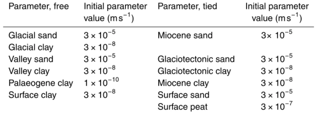
– The horizontal hydraulic conductivities of all zones of the 11 hydrostratigraphic cluster models. Figure 5 shows sensitivity toK of the zones of the 5-cluster model.

K of the zones are unknown; hence all K values have been calibrated. Vertical

K values are tied to horizontalK with an anisotropy factor of 10. Initial horizontal

5

K values are 10−4_{, 10}−6 _{or 10}−8_{m s}−1 _{depending on mean clay fraction value of} a zone.

Storage parameters were set to a priori values and not calibrated.

Calibration is performed using the Marquardt–Levenberg local search optimization implemented in PEST (Doherty, 2005). Observations are 632 hydraulic heads from

10

132 well filters and daily stream discharge time series from three gauging stations, see Fig. 3. Observation variances are estimated, and, in the absence of information, observation errors were assumed to be uncorrelated. Objective functions for head and discharge have been scaled to balance contributions to the total objective function.

The aggregated objective function, Φ_{, shown in Eq. (1) is the sum of the scaled}

15

objective function for head and discharge. The subjective weight,w_s, was determined through trial and error by starting numerous calibration runs;w_s was chosen to be 0.8.

Φ =_w s

Nh

X

i=₁ h

sim,i−hobs,i

σ_i

2

+₍₁₋_w s)

N_q

X

i=₁ q

sim,i−qobs,i

σ_i

2

(1)

Hydraulic head observation errors are determined following the guidelines following Henriksen et al. (2003). They suggest an error budget approach which accounts for

20

contributions from (1) the measurement (e.g. with dip meter), (2) inaccuracy in vertical referencing of wells, (3) interpolation between computational nodes to observation well location; and (4) heterogeneity that is not represented in the lumped computational grid. The total error expresses the expected uncertainty between observation and cor-responding simulation. The approach for estimating these uncertainties can be found

25

(14)

HESSD

12, 1555–1598, 2015

P. A. Marker et al.

Title Page

Tables Figures

◭ ◮

Back Close

Full Screen / Esc

Discussion

P

a

per

|

Discussion

P

a

per

|

Discussion

P

a

per

|

Discussion

P

a

per

|

Uncertainty of stream discharges is mainly due to translation from water stages to discharge (daily mean discharges). Uncertainties originate from infrequent calibra-tion of rating curve, ice forming on streams and especially stream bank vegetacalibra-tion (Raaschou, 1991). Errors can be as large as 50 %. Blicher (1991) estimates errors of 5 and 10 % on the water stage measurement and rating curve respectively. In cases

5

of very low stream flows (1 L s−1_{) Christensen et al. (1998) assigned a SD of 200 %} while flow of 50 and 5–10 L s−1 _{are assigned SD of 5 and 25 % respectively. We have} assigned an error of 20 % to all stream discharge observations.

2.5 Benchmarking hydrostratigraphic cluster models

The performance of the hydrological model based on the cluster model

hydrostratig-10

raphy has been benchmarked against the hydrological performance using a reference geological model (He et al., 2015). The reference geological model is based on geo-logical interpretation and AEM data. The study area was subdivided into seven major geological elements, based on geological interpretation. The seven elements are the Palaeogene clay, the Miocene, Boulstrup tunnel valley, three glacial sequences, and

15

a glaciotectonic complex. By collapsing the three glacial sequences into one glacial element, four hydrogeological elements were defined; the Miocene, Boultrup tunnel valley, the glacial, and the glaciotectonic complex. He et al. (2014) performed a geo-statistical analysis with TProGS (Carle and Fogg, 1996) on the lithological information and AEM data in the Miocene element to determine a sand-clay cut-off_{value for}

geo-20

physical resistivities. This cut-off_{value was used to subdivide each of the four elements} into units of sand and clay. Surface geology is characterized by a clay, sand and peat unit. The horizontal distribution of clay, sand and peat is taken from the Danish Na-tional Water Resources Model (Højberg et al., 2010). Because of problems with drying filters in groundwater abstraction wells, a material with horizontal and vertical hydraulic

25

(15)

de-HESSD

12, 1555–1598, 2015

P. A. Marker et al.

Title Page

Tables Figures

◭ ◮

Back Close

Full Screen / Esc

Discussion

P

a

per

|

Discussion

P

a

per

|

Discussion

P

a

per

|

Discussion

P

a

per

|

scribed previously. The only diff_{erence between the hydrological models and the} cali-brations are the parameterization (structures and values) of the saturated zone. As for the cluster models the Palaeogene clay surface elevation defines the lower boundary of the hydrological model. A vertical anisotropy of 1/10 is assumed for all geological units. Calibration parameters of the reference model are shown in Table 1. Specific

5

yield values are fixed 0.05 and 0.2 for clay and sand deposits respectively, and specific storage is fixed at 5×10−5.

3 Results and discussion

First we show results for the hydrological performance of 11 hydrostratigraphic cluster models consisting of 1–11 zones. Secondly details of the cluster analysis for the case

10

of a 5-cluster hydrostratigraphy are shown. Finally the results of benchmarking with the reference model are presented through comparison of observed and simulated state variables.

3.1 Calibration and validation of hydrological model

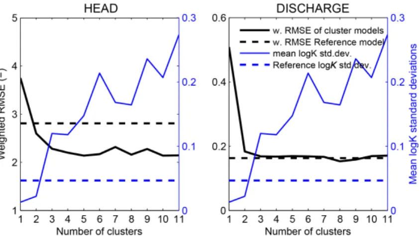
Figure 6 shows the weighted RMSE of models consisting of hydrostratigraphic cluster

15

model of 1–11 zones. Values are shown for head and discharge in separate figures. The 1-cluster model is a homogeneous representation of the subsurface resulting in a uniform K field. The 1-cluster model represents a situation where we have no in-formation about the subsurface. Increasing the number of clusters to represent the subsurface successively adds more information from geophysical and lithological data

20

to the calibration problem. Horizontal dashed lines indicate weighted RMSE of the ref-erence model. The weights used to calculate weighted RMSE are the same weights as used in Eq. (1).

Head and discharge contribute by approximately 2/3 and 1/3 of the total objective function. From the 1-cluster to the 2-cluster model, weighted RMSE for discharge is

(16)

HESSD

12, 1555–1598, 2015

P. A. Marker et al.

Title Page

Tables Figures

◭ ◮

Back Close

Full Screen / Esc

Discussion

P

a

per

|

Discussion

P

a

per

|

Discussion

P

a

per

|

Discussion

P

a

per

|

reduced by more than a factor 2. No significant improvement of the fit to discharge data is observed for more than 2 clusters. Fit to head data improves almost by a factor of 2 from the 1-cluster to the 2-cluster model. Improvement of the fit to head data continues up to the 5-cluster representation of the subsurface. Improvements are a factor of 3 from the 1-cluster to the 5-cluster model. Beyond the 5-cluster model, the fit to head

5

observations stagnates. The 7-cluster and 9-cluster hydrostratigraphic models perform worse than the 3-cluster model. The 8-, 10-, and 11-cluster models obtain an equally good or better fits to head data compared to the 5-cluster model.

The blue lines in Fig. 6 illustrate mean SD on log(K) values of the cluster models and reference model respectively, based on the post-calibration SD of log(K) for each

10

K zone. The mean SD of the reference model is 0.046, and corresponds to that of the 2- and 3-cluster models. Beyond the 4- and 5-cluster models the precision of the esti-matedK values decrease. The mean SD on log(K) for the 4- and 5-cluster models are 0.12 and 0.15. The corresponding widths of the 95 % confidence intervals are between 15 and 90 % of the estimatedK value for 3 out of 4 zones and 3 out of 5 zones,

re-15

spectively. Beyond the 5-cluster model mean SD on log(K) are between 0.17 and 0.27, and corresponding width of the 95 % confidence intervals are largely above 100 % for all but two zones.

With the combined information from weighted RMSE values and SD on log(K) we are able to address over-parameterisation. The results indicate that we obtain good fit

20

to observations without over-parameterisation with a 4- to 5-cluster hydrostratigraphic model.

In this paper, we have discussed the performance of the cluster models as a mea-sure of fit to hydraulic head and stream discharge observations. Integrated hydrological models are typically used to predict transport, groundwater age, and capture zones,

25

(17)

HESSD

12, 1555–1598, 2015

P. A. Marker et al.

Title Page

Tables Figures

◭ ◮

Back Close

Full Screen / Esc

Discussion

P

a

per

|

Discussion

P

a

per

|

Discussion

P

a

per

|

Discussion

P

a

per

|

The hydrostratigraphic models are constructed under the assumption that subsur-face structures governing groundwater flow can be captured by structural information contained in clay fraction values (derived from lithological borehole data) and geophys-ical resistivity values. If this is true, an asymptotic improvement of the data fit would be expected for increasing cluster numbers. However, as shown in Fig. 6, this is not

5

strictly the case: weighted RMSE of the 7-cluster and 9-cluster models is higher than weighted RMSE of the 3-cluster, 6-cluster and 8-cluster models, respectively. The likely explanation is that increasing number of clusters does not correspond to pure cluster sub-division, but also to relocation of cluster interfaces in the 3-D model space. We expect the difference in hydrological performance to be due to changes in interface

10

configuration.

It is well-known that an unsupervisedk-means clustering algorithm does not result in unique solution, due to choice of initial (and unknown) cluster centroids. We have sam-pled the solution spaces (200 samples) of the eleven cluster models. Clustering the principal components of geophysical resistivity data and clay fraction values into 1 to

15

5 clusters gives unique solutions. Clustering the principal components of geophysical resistivity data and clay fraction values into 6 to 11 clusters results in three or more so-lutions. The non-unique solutions however have diff_{erent objective functions (squared} Euclidean distance between points and centroids). In all cases the cluster model with the lowest objective function was chosen as the best solution.

20

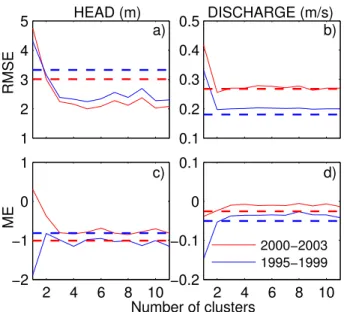
Figure 7 shows RMSE and mean errors for calibration and validation periods for all 11 cluster models and the reference model. Horizontal dotted lines are reference model performances. Data used to calculate the statistics are a temporally split sample from 35 wells, which have observations both in the calibration and validation period, and the discharge is for stations 270002 and 270003.

25

(18)

HESSD

12, 1555–1598, 2015

P. A. Marker et al.

Title Page

Tables Figures

◭ ◮

Back Close

Full Screen / Esc

Discussion

P

a

per

|

Discussion

P

a

per

|

Discussion

P

a

per

|

Discussion

P

a

per

|

head, Fig. 7c, are lower and higher for the reference model and the cluster models respectively. The hydrological models analysed in this study generally under-simulate the average discharge.

From Fig. 7a and c it appears that the cluster models for 3-4-5 clusters perform better than the reference model with respect to RMSE head, while they have equal

5

performance for ME head. Recalling that the reference model and the 5-cluster model have respectively 6 and 5 degrees of freedom in the hydrological model calibration, this indicates the diff_{erence in spatial patterns of the two models.}

3.2 The cluster model

Figure 8 presents histograms of clay fraction values and resistivity values and how the

10

values are represented in the five clusters, which was chosen to be the optimal num-ber. Counts are shown as percentages of total number of pixels in the domain. The histograms in Fig. 8 show that the clay fraction attribute separates high resistivity/low clay fraction (sandy sediments) from other high-resistivity portions of the domain, while the resistivity attribute separates low resistivity/high clay fraction (clayey sediments)

15

from other high clay-fraction portions. High resistivity/low clay fraction values are rep-resented by clusters 1, 3 and 4 and low resistivity/high clay fraction are reprep-resented by clusters 2 and 5 (see Fig. 8a).

Figure 9 shows the data cloud that forms the basis of the clustering. The data cloud is binned into 300 bins in each dimension and the colour of the cloud shows the bin-wise

20

data density. We see that cluster boundaries appear as straight lines in the attribute space. Values with a low resistivity and corresponding high clay fraction, mainly clusters 2 and 5, populate more than half of the domain. Clay is expected to dominate this part of the domain.

The results of the cluster analysis are presented with respect to geophysical

resis-25

(19)

HESSD

12, 1555–1598, 2015

P. A. Marker et al.

Title Page

Tables Figures

◭ ◮

Back Close

Full Screen / Esc

Discussion

P

a

per

|

Discussion

P

a

per

|

Discussion

P

a

per

|

Discussion

P

a

per

|

are inversely correlated. This corresponds to the situation where a clay fraction of 1 co-incides with a low resistivity value, and vice versa for clay fraction values of 0 and high resistivities. This is the information that we expect, i.e. our understanding of how geo-physical resistivities relate to lithological information as represented by our translator function (defined under the assumption that variation in geophysical resistivities with

5

respect to lithological information depends on the presence of clay materials). Thus the first principal component is the “clay” information in the geophysical resistivities. The second PC is less straight forward to interpret. Ideally, the second PC represents the data pairs where the resistivity response isnotdominated or explained by litholog-ical clay material. This might reflect a situation where a low resistivity value – and its

10

associated low clay fraction value – is a result of a sandy material with a high pore-water electrical conductivity due to elevated dissolved ion concentrations. The second PC can also be a result of the CF-conceptualisation. Clay till, categorized as “clay” in the CF-inversion, can have electrical resistivities up to 60Ω_{m (Jorgensen et al., 2005;} Sandersen et al., 2009), which will yield a high clay fraction coinciding with a relatively

15

high geophysical resistivity.

Electromagnetic methods are sensitive to the electrical resistivity of the formation, which is commonly dominated by clay mineral content, dissolved ions in the pore water and saturation. Groundwater quality data is available at numerous sites in the domain. Pore-water electrical conductivity (EC) values were gathered from the coast and inland

20

following the tunnel valley. From the coast and 12 km inland values are stable around 50–70 mS m−1 _{at 28 wells with varying filter depths. Four outliers with EC ranging} be-tween 120 and 250 mS m−1 _{were identified at various locations and depths. No trend} due to salinity from the coast was identified. In theory variations in formation electrical resistivity that arenotdue to lithological changes will implicitly be taken into account by

25

(20)

HESSD

12, 1555–1598, 2015

P. A. Marker et al.

Title Page

Tables Figures

◭ ◮

Back Close

Full Screen / Esc

Discussion

P

a

per

|

Discussion

P

a

per

|

Discussion

P

a

per

|

Discussion

P

a

per

|

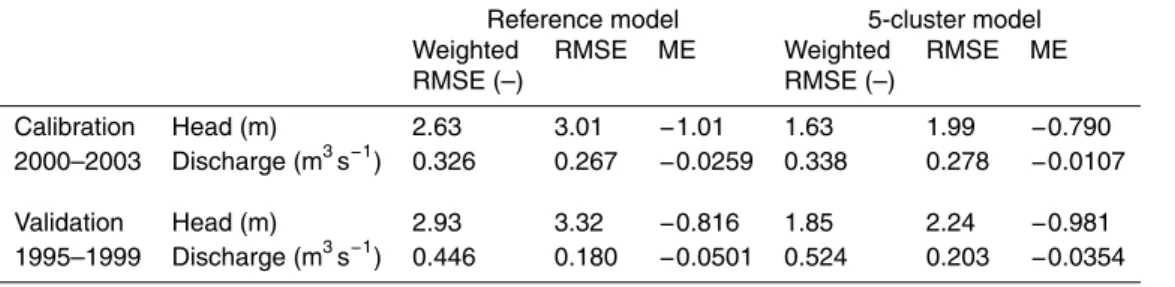
3.3 Benchmarking hydrological performance

Table 2 gives an overview of how the performance of the two models compare. The fit to discharge data of the two models is comparable. The weighted RMSE for discharge is below 1, indicating that discharge is over-fitted. The SD of discharge is 20 % of the observation, which is a conservative definition. As presented in the methods section

er-5

rors may vary between 5–50 %. The 1995–1999 hydrograph and scatter plot in Fig. 10 for the 270002 gauging station show good fit to data. Peak and low flows are fitted, but baseflow recession is generally not matched very well. At gauging station 27003 the models fail to capture dynamics and relative magnitudes of the observations. Peak as well as low flows are under-simulated, which is clearly demonstrated in the scatter plot

10

for station 270003 in Fig. 10.

The hydraulic head performance statistics in Table 2 show an improved performance of the 5-cluster model over the reference model: the calibration period RMSE/ME for the reference and 5-cluster model respectively is 3.01/−1.01 and 1.99/−0.790 m. Weighted RMSE for the reference model is 2.63 and 2.93, while weighted RMSE for

15

the 5-cluster model is 1.63 and 1.85. The reference model thus is 2–3 SD from fitting data, while the 5-cluster model is 1–2 SD from fitting data. Assuming head observation error estimates are correct, this indicates model deficiencies such as structural errors and/or forcing data errors. The outliers in the simulated head from the reference model, Fig. 11 red diamonds, are from three wells in the elevated south-western part of the

20

domain. Recalculating performance statistics without the outliers gives RMSE and ME of 2.45 and−0.647 m. Figure 11 shows that the largest differences in simulated heads between the two models are for hydraulic head below 20 m. These observations rep-resent the tunnel valley aquifers (see also Fig. 12a and b). Results indicate that the 5-cluster model performs better in the tunnel valley than the reference model.

25

(21)

HESSD

12, 1555–1598, 2015

P. A. Marker et al.

Title Page

Tables Figures

◭ ◮

Back Close

Full Screen / Esc

Discussion

P

a

per

|

Discussion

P

a

per

|

Discussion

P

a

per

|

Discussion

P

a

per

|

and groundwater overall flows towards the sea. The reference model simulates higher heads (Fig. 12b) in the tunnel valley compared to the 5-cluster model. Figure 12c and d show errors (obs-sim) between observed and simulated heads for 1995–1999. Errors in the elevated terrain towards west are similar for the two models, whereas the reference model has larger errors (over-simulates head) in the tunnel valley compared to the

5

5-cluster model.

3.4 Advantages and limitations

We have presented a method for automatic generation of hydrostratigraphic models from AEM and lithological data for groundwater model applications. Other automatic methods of integrating AEM data into geological models are geostatistical methods

pre-10

sented by e.g. Gunnink et al. (2012), using artificial neural networks, or He et al. (2014), using transition probabilities.

A limitation of performing automatic integration of AEM is that eff_{ects of saturation,} water quality, depth and material dependent resolution, and vertical shielding eff_ects are misinterpreted, and wrongly interpreted as geological structural information. These

15

eff_{ects may be identified by a geologist during the modelling process. AEM data can be} integrated into geological models using cognitive methods, for example as presented by Jørgensen et al. (2013), who provide an insightful discussion of the pros and cons of automatic vs. cognitive geological modelling from AEM data.

Geological knowledge, which can be incorporated into cognitive geological models

20

(Royse, 2010; Scharling et al., 2009; Sharpe et al., 2007), cannot be included in auto-matically generated models. Geological knowledge may identify continuity/discontinuity of geological layers, or discriminate materials based on stratigraphy or depositional environment. For regional scale groundwater flow, characterisation of sedimentation patterns and sequences may not be relevant, but at smaller scales this information is

25

valuable for transport modelling.

(22)

HESSD

12, 1555–1598, 2015

P. A. Marker et al.

Title Page

Tables Figures

◭ ◮

Back Close

Full Screen / Esc

Discussion

P

a

per

|

Discussion

P

a

per

|

Discussion

P

a

per

|

Discussion

P

a

per

|

sets. This is not possible in practice for cognitive methods due to spatial complexity and AEM data amounts. Also reproducibility and especially possibility of uncertainty quantification of the hydrostratigraphic cluster model are important features. For hydro-logical applications hydrostratigraphic model uncertainty, and the resulting hydrohydro-logical prediction uncertainty, has great value. Cognitive geological model uncertainty is diffi

-5

cult to quantify.

4 Conclusion

We have presented an automated workflow to parameterize and calibrate a large-scale integrated hydrological model based on AEM and borehole data. The result is a competitive hydrological model that performs equally good or even better than the

10

reference geological model. From geophysical resistivity data and clay fraction values we delineate hydrostratigraphic zones, whose hydrological properties are estimated in a hydrological model calibration. The method allows for semi-automatic generation of reproducible hydrostratigraphic models. Reproducibility is naturally inherent as the method is data-driven and thus, to a large extent, also objective.

15

The number of zones in the hydrostratigraphic model must be determined as part of the cluster analysis. We have proposed that hydrological data, through hydrological calibration and validation, guide this choice. Based on fit to head and discharge obser-vation and calibration parameter SD, results indicate that the 4- and 5-cluster models give the optimal performance.

20

Distributed groundwater models are used globally to manage groundwater sources. Today large-scale AEM data sets are acquired for mapping groundwater re-sources on a routine basis around the globe. There is a lack of knowledge on how to incorporate the results of these surveys into groundwater models. We believe the proposed method has potential to solve this problem.

(23)

HESSD

12, 1555–1598, 2015

P. A. Marker et al.

Title Page

Tables Figures

◭ ◮

Back Close

Full Screen / Esc

Discussion

P

a

per

|

Discussion

P

a

per

|

Discussion

P

a

per

|

Discussion

P

a

per

|

Appendix A: Observation errors

Hydraulic head observation errors have been estimated using an error budget;

σ_total2 =_σ2

meas+σelev2 +σ 2 int+σ

2

hetereo+σ 2 unknown.

Quantitative estimates of the diff_{erent error sources are to a large extent based on data} from the Danish Jupiter database.

5

Head measurements are typically carried out with dip-meter, and occasionally pres-sure transducers are used. Information about which meapres-surement technique has been used for the individual observations is not clear from the Jupiter database. It is as-sumed that dip-meters have been used andσ_meas has been determined to be 0.05 m for all observations.

10

Well elevations are referenced using diff_{erent techniques. The elevation can be} de-termined from a 1 : 25 000 topographic map, by levelling or by diff_{erential GPS. The} inaccuracies for using topographic maps and DGPS measurements are in the order of respectively 1–2 m and centimetres. The Jupiter database can have information about the referencing techniques, but this information is rarely supplied. An implicit

infor-15

mation source is the number of decimal places the elevations have in the database. Elevation information is supplied with 0, 1 or 2 decimal places. For the wells where the reference technique is available (checked for cases with topographic map and DGPS only) the decimal places reflect accuracy of the referencing technique used. From this information decimal places of 0, 1 and 2 have been associated withσ_elev of 2, 1 and

20

0.1 m respectively.

Errors due to interpolation depend on horizontal discretization of the hydrological model and the hydraulic gradient. Sonnenborg and Henriksen (2005, chapter 12) sug-gest it be estimated as σ_int=0.5·∆x·J, where ∆x is horizontal discretization and J is hydraulic gradient. The model domain has been divided into three groups for which

25

(24)

HESSD

12, 1555–1598, 2015

P. A. Marker et al.

Title Page

Tables Figures

◭ ◮

Back Close

Full Screen / Esc

Discussion

P

a

per

|

Discussion

P

a

per

|

Discussion

P

a

per

|

Discussion

P

a

per

|

melt water sediments; and the Palaeogene tunnel valley. Hydraulic gradients of the Miocene/Glacial west and the Palaeogene tunnel valley are between 0.001–0.002. The Miocene/Glacial area and the Palaeogene tunnel valley areas were thus considered as one withσintof 0.07 m. The glacial tectonic area has an estimated hydraulic gradient of 0.01 and thus associated withσ_intof 0.6 m.

5

Within-cell (hydrological model grid) heterogeneity aff_{ecting hydraulic head was} esti-mated using data from eight wells that are located within the same hydrological model grid. Temporally coinciding head observations from the period 2001 and 2002 were used. The error is evaluated as the SD of a linear plane fitted through the observed heads at the eight boreholes. This has been done for three dates, which gives a mean

10

σ_hetereoof 0.53 m.

σ_unknownwas set to 0.5 m.

Acknowledgements. This paper was supported by HyGEM, Integrating geophysics, geology, and hydrology for improved groundwater and environmental management, Project no. 11-116763. The funding for HyGEM is provided by The Danish Council for Strategic Research.

15

We are thankful for the support and data provided by the NiCA research project (funded by The Danish Council for Strategic Research under contract no. DSF 09-067260), including SkyTEM data and the integrated hydrological model for Norsminde study area.

References

Abbott, M. B., Bathurst, J. C., Cunge, J. A., O’Connell, P. E., and Rasmussen, J.: An introduction

20

to the European hydrological system – Systeme Hydrologique Europeen, “SHE”, 2: Structure of a physically-based, distributed modelling system, J. Hydrol., 87, 61–77, doi:10.1016/0022-1694(86)90115-0, 1986.

Auken, E. and Christiansen, A. V: Layered and laterally constrained 2D inversion of resistivity data, Geophysics, 69, 752–761, doi:10.1190/1.1759461, 2004.

25

(25)

HESSD

12, 1555–1598, 2015

P. A. Marker et al.

Title Page

Tables Figures

◭ ◮

Back Close

Full Screen / Esc

Discussion

P

a

per

|

Discussion

P

a

per

|

Discussion

P

a

per

|

Discussion

P

a

per

|

Auken, E., Christiansen, A. V., Kirkegaard, C., Fiandaca, G., Schamper, C., Behrooz-mand, A. A., Binley, A., Nielsen, E., Eff_{ersø, F., Christensen, N. B., Sørensen, K., Foged, N.,}

and Vignoli, G.: An overview of a highly versatile forward and stable inverse algorithm for airborne, ground-based and borehole electromagnetic and electric data, Explor. Geophys., doi:10.1071/EG13097, in press, 2014.

5

Bedrosian, P. A., Maercklin, N., Weckmann, U., Bartov, Y., Ryberg, T., and Ritter, O.: Lithology-derived structure classification from the joint interpretation of magnetotelluric and seismic models, Geophys. J. Int., 170, 737–748, doi:10.1111/j.1365-246X.2007.03440.x, 2007. Beven, K.: Changing ideas in hydrology – the case of physically-based models, J. Hydrol., 105,

157–172, doi:10.1016/0022-1694(89)90101-7, 1989.

10

Blicher, A. S.: Usikkerhed på bearbejdning af data fra vandføringsstationer, Publication nr. 1 from Fagdatacenter for Hydrometriske Data, Hedeselskabet, Viborg, 1991.

Borgesen, C. and Schaap, M.: Point and parameter pedotransfer functions

for water retention predictions for Danish soils, Geoderma, 127, 154–167, doi:10.1016/j.geoderma.2004.11.025, 2005.

15

Bosch, J. H. A., Bakker, M. A. J., Gunnink, J. L., and Paap, B. F.: Airborne electromagnetic mea-surements as basis for a 3D geological model of an Elsterian incision, Hubschrauberelek-tromagnetische Messungen als Grundlage für das geologische 3D-Modell einer glazialen Rinne aus der Elsterzeit, Z. Dtsch. Ges. Geowiss., 160, 249–258, doi:10.1127/1860-1804/2009/0160-0258, 2009.

20

Carle, S. F. and Fogg, G. E.: Transition probability-based indicator geostatistics, Math. Geol., 28, 453–476, doi:10.1007/BF02083656, 1996.

Christensen, S., Rasmussen, K. R., and Moller, K.: Prediction of regional ground water flow to streams, Ground Water, 36, 351–360, doi:10.1111/j.1745-6584.1998.tb01100.x, 1998. Christiansen, A. V. and Auken, E.: A global measure for depth of investigation, Geophysics, 77,

25

WB171–WB177, doi:10.1190/geo2011-0393.1, 2012.

Christiansen, A. V., Auken, E., Foged, N., and Sorensen, K. I.: Mutually and laterally constrained inversion of CVES and TEM data: a case study, Near Surf. Geophys., 5, 115–123, 2007. Christiansen, A. V., Foged, N., and Auken, E.: A concept for calculating accumulated clay

thick-ness from borehole lithological logs and resistivity models for nitrate vulnerability

assess-30

ment, J. Appl. Geophys., 108, 69–77, doi:10.1016/j.jappgeo.2014.06.010, 2014.

(26)

HESSD

12, 1555–1598, 2015

P. A. Marker et al.

Title Page

Tables Figures

◭ ◮

Back Close

Full Screen / Esc

Discussion

P

a

per

|

Discussion

P

a

per

|

Discussion

P

a

per

|

Discussion

P

a

per

|

DHI: MIKE SHE User Manual: Reference Guide, Hørsholm, Denmark, 2012.

Doherty, J.: PEST: Model-Independent Parameter Estimation, User Manual, 5th Edn., Brisbane, QLD, Australia, 2005.

Foged, N., Marker, P. A., Christansen, A. V., Bauer-Gottwein, P., Jørgensen, F., Høyer, A.-S., and Auken, E.: Large-scale 3-D modeling by integration of resistivity models and borehole

5

data through inversion, Hydrol. Earth Syst. Sci., 18, 4349–4362, doi:10.5194/hess-18-4349-2014, 2014.

Gallardo, L. A.: Characterization of heterogeneous near-surface materials by joint 2D inversion of dc resistivity and seismic data, Geophys. Res. Lett., 30, 1658, doi:10.1029/2003GL017370, 2003.

10

GEUS: Danish national geological and hydrological database, JUPITER, n.d.

Di Giuseppe, M. G., Troiano, A., Troise, C., and De Natale, G.:k-Means clustering as tool for multivariate geophysical data analysis. An application to shallow fault zone imaging, J. Appl. Geophys., 101, 108–115, doi:10.1016/j.jappgeo.2013.12.004, 2014.

Gräbe, A., Rödiger, T., Rink, K., Fischer, T., Sun, F., Wang, W., Siebert, C., and Kolditz, O.:

15

Numerical analysis of the groundwater regime in the western Dead Sea escarpment, Is-rael+_{West Bank, Environ. Earth Sci., 69, 571–585, doi:10.1007/s12665-012-1795-8, 2012.}

Graham, D. N. and Butts, M. B.: Flexible integrated watershed modeling with MIKE SHE, in: Watershed Models, edited by: Singh, V. P. and Frever, D. K., CRC Press, Boca Raton, 245– 272, 2005.

20

Greve, M. H., Greve, M. B., Bøcher, P. K., Balstrøm, T., Breuning-Madsen, H., and Krogh, L.: Generating a Danish raster-based topsoil property map combining choropleth maps and point information, Geogr. Tidsskr., 107, 1–12, doi:10.1080/00167223.2007.10649565, 2007. Gunnink, J. L., Bosch, J. H. A., Siemon, B., Roth, B., and Auken, E.: Combining ground-based

and airborne EM through Artificial Neural Networks for modelling glacial till under saline

25

groundwater conditions, Hydrol. Earth Syst. Sci., 16, 3061–3074, doi:10.5194/hess-16-3061-2012, 2012.

Haber, E. and Oldenburg, D.: Joint inversion: a structural approach, Inverse Probl., 13, 63–77, doi:10.1088/0266-5611/13/1/006, 1997.

Hansen, A. L., Refsgaard, J. C., Christensen, B. S. B., and Jensen, K. H.: Importance of

includ-30

(27)

HESSD

12, 1555–1598, 2015

P. A. Marker et al.

Title Page

Tables Figures

◭ ◮

Back Close

Full Screen / Esc

Discussion

P

a

per

|

Discussion

P

a

per

|

Discussion

P

a

per

|

Discussion

P

a

per

|

Härdle, W. K. and Simar, L.: Applied multivariate statistical analysis, 3rd Edn., Springer, Heidel-berg, 2012.

He, X., Sonnenborg, T. O., Jørgensen, F., Høyer, A.-S., Møller, R. R., and Jensen, K. H.: Ana-lyzing the eff_{ects of geological and parameter uncertainty on prediction of groundwater head}

and travel time, Hydrol. Earth Syst. Sci., 17, 3245–3260, doi:10.5194/hess-17-3245-2013,

5

2013.

He, X., Koch, J., Sonnenborg, T. O., Jørgensen, F., Schamper, C., and Christian Refsgaard, J.: Transition probability-based stochastic geological modeling using airborne geophysical data and borehole data, Water Resour. Res., 50, 3147–3169, doi:10.1002/2013WR014593, 2014.

10

He, X., Henriksen, H. J., and Stisen, S.: Designing an end-user driven real-time hydrological early warning system in denmark, Hydrol. Res., in review, 2015.

Henriksen, H. J., Troldborg, L., Nyegaard, P., Sonnenborg, T. O., Refsgaard, J. C., and Mad-sen, B.: Methodology for construction, calibration and validation of a national hydrological model for Denmark, J. Hydrol., 280, 52–71, doi:10.1016/s0022-1694(03)00186-0, 2003.

15

Herckenrath, D., Fiandaca, G., Auken, E., and Bauer-Gottwein, P.: Sequential and joint hy-drogeophysical inversion using a field-scale groundwater model with ERT and TDEM data, Hydrol. Earth Syst. Sci., 17, 4043–4060, doi:10.5194/hess-17-4043-2013, 2013.

Hill, M. C.: Eff_{ective Groundwater Model Calibration: With Analysis of Data, Sensitives,}

Predic-tions, and Uncertainty, Wiley-Interscience, Hoboken, NJ, 2007.

20

Hinnell, A. C., Ferre, T. P. A., Vrugt, J. A., Huisman, J. A., Moysey, S., Rings, J., and Kowalsky, M. B.: Improved extraction of hydrologic information from geophysical data through coupled hydrogeophysical inversion, Water Resour. Res., 46, W00D40, doi:10.1029/2008wr007060, 2010.

Højberg, A. L., Nyegaard, P., Stisen, S., Troldborg, L., Ondracek, M., and Christensen, B. S. B.:

25

DK-model2009, Modelopstilling og Kalibrering for Midtjylland, GEUS, København, 2010. Hotelling, H.: Analysis of a complex of statistical variables into principal components, J. Educ.

Psychol., 24, 417–441, doi:10.1037/h0071325, 1933.

Høyer, A.-S., Lykke-Andersen, H., Jørgensen, F., and Auken, E.: Combined interpretation of SkyTEM and high-resolution seismic data, Phys. Chem. Earth Pt. A/B/C, 36, 1386–1397,

30