www.scielo.br/rbg
A WELL-LOG REGRESSION ANALYSIS FOR P-WAVE VELOCITY PREDICTION
IN THE NAMORADO OIL FIELD, CAMPOS BASIN
Fabr´ıcio de Oliveira Alves Augusto and Jorge Leonardo Martins
Recebido em 13 abril, 2009 / Aceito em 19 janeiro, 2010 Received on April 13, 2009 / Accepted on January 19, 2010
ABSTRACT.Geophysical well log measurements are key information for the development of oil and gas reservoirs. However, the absence of a certain fundamen-tal well log, for instance, the compressional-wave (P-wave) sonic log, prevents the application of specific risk-assessment techniques. Therefore, the application of methodologies for estimating log records absent in wells is of great importance in the reservoir characterization and development procedures. In this paper, we use the regression analysis methodology for estimating P-wave sonic log measurements. Effective porosity, shaliness and electrical resistivity are established, individually or in a combined way, as the parameters for describing P-wave velocity variation in Namorado oil field, Campos basin. Two general equations provide 28 empirical models with potential use in estimating P-wave velocity variation from well log measurements. Application of least-squares technique leads to the determination of lithology-related regression coefficients at the surroundings of two wells chosen for verifying the empirical models. The results show the equivalence of both general equations used for obtaining empirical models for P-wave velocity estimation. As confirmation of papers published previously, empirical models assuming effective porosity and/or shaliness as dependence parameters play a fundamental role in the prediction of velocity variation. Nevertheless, the velocity calibration process exhibits high stability for empirical models in which electrical resistivity is used as an additional dependence parameter.
Keywords: geophysical well logs, regression analysis, P-wave velocity estimation, Namorado reservoir.
RESUMO.Registros de perfilagem geof´ısica de poc¸os s˜ao informac¸˜oes cruciais para o desenvolvimento de reservat´orios de petr´oleo e g´as. Entretanto, a ausˆencia de qualquer perfil geof´ısico fundamental, por exemplo, o perfil sˆonico de ondas compressionais (ondas P), impede a aplicac¸˜ao de t´ecnicas espec´ıficas de avaliac¸˜ao de risco. Portanto, a aplicac¸˜ao de metodologias para estimativa de registros de perfis ausentes em poc¸os ´e de grande importˆancia nos procedimentos de caracterizac¸˜ao e desenvolvimento de reservat´orios. Neste artigo, usamos a metodologia de an´alise de regress˜ao para estimar registros de perfil sˆonico de ondas P. Porosidade efetiva, argilosidade e resistividade el´etrica s˜ao estabelecidos, individualmente ou de forma combinada, como os parˆametros para descrever a variac¸˜ao da velocidade de ondas P no campo de Namorado, bacia de Campos. Duas equac¸˜oes gerais fornecem 28 modelos emp´ıricos com uso potencial na estimativa da variac¸˜ao de velocidade de ondas P a partir de registros de perfis de poc¸os. A aplicac¸˜ao da t´ecnica de m´ınimos quadrados conduz `a determinac¸˜ao dos coeficientes das regress˜oes relacionados `a litologia nas imediac¸˜oes de dois poc¸os escolhidos para verificar os modelos emp´ıricos. Os resultados mostram a equivalˆencia de ambas equac¸˜oes gerais usadas na obtenc¸˜ao dos modelos emp´ıricos para estimativa de velocidade de ondas P. Como confirmac¸˜ao de artigos publicados anteriormente, modelos emp´ıricos que assumem porosidade efetiva e/ou argilosidade como parˆametros da dependˆencia desempenham papel fundamental na descric¸˜ao da variac¸˜ao da velocidade. Entretanto, o processo de calibrac¸˜ao da velocidade exibe alta estabilidade para modelos emp´ıricos nos quais a resistividade el´etrica ´e utilizada como um parˆametro adicional da dependˆencia.
Palavras-chave: perfis geof´ısicos de poc¸os, an´alise de regress˜ao, estimativa de velocidade de ondas P, reservat´orio Namorado.
INTRODUCTION
The geophysical development of an oil and gas field relies on characterizing the variation of petrophysical properties through-out the sedimentary interval containing the reservoirs (Archie, 1950). In this way, laboratory measurements on core plugs, inter-pretation of geophysical well logs and inversion of seismic attri-butes provide valuable estimates of reservoir physical properties. Integration of these distinct methodologies is the best approach to determine uncertainties in the predictions, with direct implica-tions on risk mitigation in drilling operaimplica-tions (Pennington, 2001). The estimation of any physical rock property implies to adopt a mathematical model. However, the selected model hardly con-tains the full set of parameters affecting the rock property under study. In general, the dependence of a given rock property is stu-died considering a parameter separately or combining relevant parameters in order to establish a corresponding mathematical model. For instance, let us take the effective-medium theory mo-del routinely used in estimating total porosity from bulk density logs (Dewan, 1983; Ellis, 1987). The model establishes depen-dence of bulk density of a porous rock on mineralogy, porosity and fluid saturation. Nevertheless, depth and/or effective pres-sure are parameters ignored in the formulation of the effective-theory model for bulk density. The degree of rock consolidation tends to increase with depth due to effective pressure. As a re-sult of ignoring those parameters in the formulation, the estima-tive of total porosity using the bulk density model becomes sim-ple. However, no correlation of the density model with the rock consolidation degree and effective pressure is allowed. A further example is the estimation of rock elastic properties (i.e., seismic velocities), which have parameter dependence yet more complex (Wyllie et al., 1956; Wyllie et al., 1958; Klimentos, 1991; Xu & White, 1995). In this case, the Voigt-Reuss and Hashin-Shtrikman effective medium theories (Watt et al., 1976) can be used for es-timating the elastic properties of mixed lithologies. However, cal-culations require detailed description on rock mineralogic cons-tituents and fluid content. Such a description demands time and is often unavailable. Alternatively, use of Biot-Gassmann equations (Toks¨oz et al., 1976; Domenico, 1976) allows calcu-lating seismic velocities for dry or saturated porous rocks at low-and high-frequency ranges. However, the incompressibilities low-and densities of the rock matrix and fluid, as well as the fractional total porosity, must be a priori known for estimating seismic velocities using Biot-Gassmann equations.
Assuming that a detailed description of the rock composition is unavailable, regression analysis methodology is usually the
procedure used in the study of parameter dependence of seismic velocities in mixed lithologies. In this instance, the investigation is highly simplified as long as individual or combined parameters (i.e., porosity, shaliness, fluid saturation, confining pressure, and others) can be considered in the seismic velocity model formu-lation. Moreover, either ultrasonic measurements in core plugs (Tosaya & Nur, 1982; Han et al., 1986; Eberhart-Phillips et al., 1989) or well log data (Raymer et al., 1980; Castagna et al., 1985; Miller & Stewart, 1990) can be the source of information used in regression analysis for parameter dependence studies of seismic velocities. In this way, interpreters gain insight for linking rock properties to attributes investigated, for instance, in oil-bearing reservoir characterization procedures (Krief et al., 1990; Murphy et al., 1991; Castagna et al., 1993).
From Wyllie’s et al. (1956, 1958) time-average equation and Raymer et al. (1980) quadratic approach, rock porosity repre-sents the main parameter affecting P-wave velocities. However, both approximations can hardly predict velocity in shaly sands-tones without significant misfits. In order to consider additio-nal parameters into the velocity dependence, a useful strategy is the application of multivariate linear regression methodologies. The papers of Tosaya & Nur (1982), Han et al. (1986) and Mil-ler & Stewart (1990) use rock porosity and shaliness to inves-tigate dependence of seismic velocities on both parameters in distinct mixed lithologies. As a result, including shaliness as a further parameter into the dependence significantly increases cor-relation with velocity measurements. In turn, Eberhart-Phillips et al. (1989) used Han’s et al. (1986) core plug data to show that effective pressure plays a significant role in predicting seismic velocities. As a common conclusion from these cited works, po-rosity and shaliness play a fundamental role in the variation of seismic velocities.
in fundamental geophysical well log measurements reveal varia-tions of physical properties in the Namorado oil field. However, the absence of the P-wave sonic log in most wells prevents cons-tructing normal-incidence synthetic seismograms required for seismic calibration procedures. Hence, the establishment of P-wave velocity models allow sonic log estimation by using cor-respondent wells at the vicinities. Oliveira & Martins (2003) per-formed similar regression study using well log measurements only from the Namorado sandstone intervals. Here we extended their regression methodology to the whole mixed lithology co-lumn representing the upper Maca´e formation. The well log re-gression methodology will be described in the next section.
METHODOLOGY
In the following, we present the steps for investigating the appli-cation of 28 empirical relations for predicting P-wave sonic logs. We selected two wells from the so-called data set “Campo Es-cola Namorado”, which is distributed by ANP/Brazil – Agˆencia Nacional do Petr´oleo, G´as Natural e Biocombust´ıveis, to Brazi-lian universities and research institutions for academic purpo-ses. The data set contains geological and geophysical well log information of more than 40 vertical wells drilled through the upper Maca´e formation. In this sedimentary interval the rocks correspond mostly to sandstones and shales of turbiditic origin, forming the offshore oil-producing Namorado field in Campos basin (Tigre & Lucchesi, 1986). Fundamental logs, i.e., gamma ray (GR), deep electrical resistivity (ILD), neutron porosity (NPHI) and bulk density (RHOB) describe variation of physical properties through the formation at the surroundings of correspondent wells, allowing identification of the oil-bearing Namorado sandstone re-servoir. The well log data set has no information on shear-wave (S-wave) sonic log, while only a limited number of wells have the corresponding P-wave sonic logs. However, at well locations where sonic logs are unavailable, linear and nonlinear empirical models for the variation of P-wave velocity in the upper Maca´e formation can be established. Based on information from the lite-rature, we assumed three main dependence parameters: the fracti-onal effective porosityφe, the fractional shale volumeVclay(i.e., shaliness) and the deep electrical resistivityRild. Conventional processing of bulk density, gamma ray and induction resistivity logs allows estimating the three mentioned dependence parame-ters. We applied the classical least-squares technique for deter-mining the regression coefficients of each empirical model. Using the correlation coefficientr, we measure the calibration step un-certainty. Below we summarize the steps of the methodology.
Selection of well logs
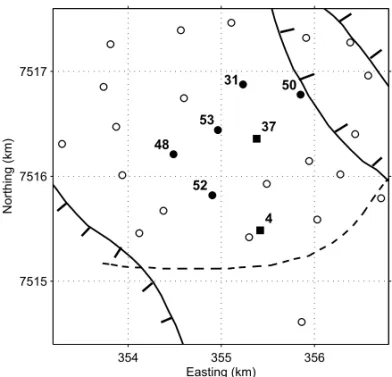
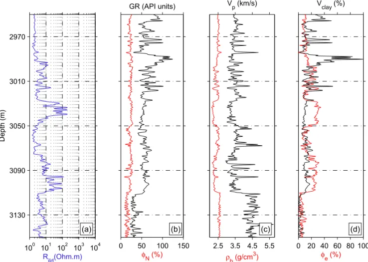
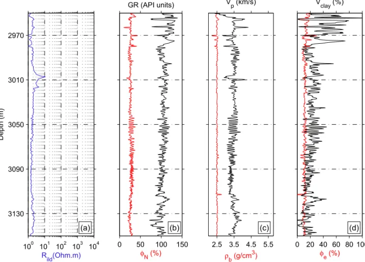
Figure 1 shows part of the structural map of the Namorado field. The reservoir resembles a mini-horst bounding by normal faults. Circles and squares denote the vertical wells drilled in the area. We selected two wells containing fundamental log measurements, including the P-wave sonic log. It corresponds to a critical infor-mation for the regression analysis and, obviously, for the calibra-tion process with the empirical models proposed. In Figure 1, filled squares indicate the selected wells, named as well-4 and well-37. The log measurements at well-4 are shown in Figure 2; the logs at well-37 are exhibited in Figure 3. In both wells, a high radioactive shale marks the top of the upper Maca´e formation as shown by the gamma-ray logs. Further inspection of Figure 2 reveals two main oil-bearing, high-porosity sandstones intervals correlating to resistivity and density anomalies. Sealing litholo-gies are mostly composites of clay and silt, with some occurrence of carbonates. The lower limit of the Maca´e formation represents calcilutites, which are easily identified in both wells by observing the abrupt variation in gamma-ray readings around 3120 m.
354 355 356
7515 7516 7517
N
o
rt
h
in
g
(km)
Easting (km) 4 37
31 50
53
52 48
Figure 1– Partial view of the structural map of Namorado oil field. Full and dashed lines represent the reservoir boundaries. Additional symbols denote well locations: circles “
◦
” correspond to well locations with incomplete and/or ab-sent logs, filled circles “•
” are wells with complete logs (excluding the P-wave sonic log), and filled boxes “” represent wells containing complete logs, in-cluding the P-wave sonic log. We refer to “ incomplete logs ” when the log shows interruptions in the readings.Shaliness estimation
100 101 102 103 104 2970
3010
3050
3090
3130
D
e
p
th
(m)
R
ild(Ohm.m)
(a)
0 50 100 150
φN (%) GR (API units)
(b)
2.5 3.5 4.5 5.5
ρb (g/cm3) V
p (km/s)
(c)
0 20 40 60 80 100
φe (%) V
clay (%)
(d)
Figure 2– Geophysical logs at well-4: (a) induction resistivity (ILD, in blue) in Ohm.m; (b) neutron porosity (NPHI, in red) in percentage and gamma-ray GR (API units); (c) bulk density (RHOB, in red) in g/cm3and the P-wave velocityv
p(km/s) profile converted from the measured sonic log; (d) effective porosity (φe, in red) and shalinessVclay, both in percentage. Application of Eqs. (1) and (3) allowed estimatingVclayandφe, respectively.
steps. In this case, Larionov (1969) presents empirical formu-las forVclayestimation based on sediment consolidation. Taking into account that the Namorado sandstone is from Tertiary age (i.e., the sediments are unconsolidated), we applied Larionov’s (1969) equation for shaliness estimation expressed as
Vclay=0.083
23.70×IGR−1. (1)
In the preceding equation, the gamma-ray indexIGRis given by
IGR= GRi −GRss GRsh−GRss
, (2)
whereGRi denotes theithgamma-ray log reading. The quanti-tiesGRssandGRshare the minimum and maximum readings in the gamma-ray log taken in the sandstone and in the shale point, respectively, in the same formation under study (Dewan, 1983; Ellis, 1987). For the sedimentary interval correspon-ding to the upper Maca´e formation,GRss≈22API units and GRsh≈125API units.
Effective porosity estimation
The following formula allows fractional effective porosityφe esti-mation from the bulk density log:
φe=φt−Vclay
ρma−ρsh ρma−ρf
, (3)
whereφtis the fractional total porosity
φt=
ρma−ρb ρma−ρf
. (4)
The parameterρbrepresents a reading in the bulk density log. As the upper Maca´e formation has quartzoze matrix, we take
100 101 102 103 104 2970
3010
3050
3090
3130
D
e
p
th
(m)
Rild(Ohm.m)
(a)
0 50 100 150
φN (%) GR (API units)
(b)
2.5 3.5 4.5 5.5
ρb (g/cm3) Vp (km/s)
(c)
0 20 40 60 80 100
φe (%) Vclay (%)
(d)
Figure 3– Geophysical logs at well-37; logs are displayed using the same color code as in Figure 2. Eqs. (1) and (3) were also respectively considered for estimating the variation of shaliness and effective porosity.
Regression analysis
The dependence of P-wave velocity in rocks is attributed to nume-rous factors. However, in order to simplify the investigation, the evidence in most published papers is the use of empirical models attempting to correlate velocity variation with specific attributes. For example, correlation of velocities with depth and geological time is presented in Faust (1951), while lithology is the parameter of the correlation in Faust (1953). Further empirical models for describing velocity variation based purely on mathematical func-tions can be found in Kaufman (1953).
In this paper, we assume the general dependence for P-wave velocity model asvp = vp(x,y,z), in which the parameters of the dependence are: effective porosity x ≡ φe, shaliness y ≡ Vclayand electrical resistivityz ≡ Rild. The choice of vpdependence was done taking the physical basis into account, and is corroborated by the results of several papers (see Han et al., 1986; Miller & Stewart, 1990; Oliveira & Martins, 2003). Thus, assumingx≡φeandy≡Vclay, we followed the work of pre-vious investigators. Moreover, the incorporation ofz≡Rildinto some empirical models led to the known dependence of P-wave velocity on fluid saturation.
The following general relations allow the investigation of li-near and nonlili-near empirical models for P-wave velocity predic-tion from well log measurements:
vpmod=VP0+VP1+VP2+VP3 (5)
and
vpmod=VP0expVP1+VP2+VP3. (6)
The above quantities VP0,VP1 ≡ VP1(x,y,z),VP2 ≡ VP2(x,y,z)andVP3≡VP3(x,y,z)are written as
VP0≡a0, (7)
VP1≡a1x+a2y+a3z, (8)
VP2≡a4x y+a5x z+a6y z, (9)
and
VP3≡a7x2+a8y2+a9z2. (10)
obtained by assuming a dependence ofvpon a single parameter, or taking more than one parameter simultaneously in the depen-dence. For instance, assuming a simple model in which the fracti-onal effective porosityφeis the only parameter of the dependence, we can write a linear model for P-wave velocity variation
vpmod=a0+a1φe. (11)
In accordance to Eq. (6), a nonlinear dependence onφecan also be provided forvp, as follows
vpmod=a0expa1φe. (12)
As in Castagna et al. (1993), we can also use the simple pa-rabolic model withy≡Vclayas the only parameter affectingvp. As a result, we obtain from Eq. (5)
vpmod=a0+a2Vclay+a8 Vclay 2
, (13)
On the other hand, Eq. (6) gives a nonlinear empirical model for
vpas a function ofVclay:
vpmod=a0expa2Vclay+a8 Vclay
2
. (14)
Besides multivariate linear models as in Han et al. (1986) and in Eberhart-Phillips et al. (1989), Eqs. (5) and (6) also allow to derive nonlinear models. For instance, assuming the parameter dependencevp≡vp(φe,Vclay,Rild), P-wave velocity can be described by the following multivariate linear model
vpmod=a0+a1φe+a2Vclay+a3Rild, (15)
or, from the general form in Eq. (6), by a multivariate nonlinear model written as
vpmod=a0expa1φe+a2Vclay+a3Rild. (16)
Two- and three-variable quadratic empirical models can also be derived from Eqs. (5) and (6). Takingx≡φeandz≡Rildas the parameters of the dependence, the P-wave velocity variation can be described as
vpmod= a0+a1φe+a3Rild+a5φeRild
+a7(φe)2+a9(Rild)2,
(17)
and
vpmod= a0expa1φe+a3Rild+a5φeRild
+a7(φe)2+a9(Rild)2.
(18)
In summary, we investigated 28 empirical models for predicting P-wave velocities using geophysical well logs. In order to deter-mine the regression coefficientsaiof the corresponding empirical model, we applied the classical least-squares technique (Lines & Treitel, 1984). We thus minimized the square of the residu-als between the measured velocityvmeasp (i.e., the readings in the P-wave sonic log) and the modeled velocityvmodp (i.e., the cho-sen empirical model). As a result, after constructing the objective functionE2≡E2(a
i)
E2= |vpmeas−vpmod|2 (19)
we operate∂E2/∂a
i ≡ 0. The sought coefficientsai are the unknowns of the resulting linear system of equations derived af-ter minimizing Eq. (19). Notice that we applied the neperian lo-garithm to both sides of Eq. (6) before operating the derivative of the objective function. Furthermore, we determined the cor-relation coefficientrin order to investigate the uncertainty in the predictions of P-wave velocities.
Calibration
In the calibration step, we focused on plotting the P-wave velocity logs at both selected wells and the empirical models provided by Eqs. (5) and (6). This procedure aimed at visually inspecting the misfits between measured and predictedvpvelocity logs. Further determination of correlation coefficients of the least-squares re-gression models and absolute residuals helped analyzing the con-fidence on the investigated empirical models.
RESULTS
Following the methodology described above, we combined the dependence parametersφe,VclayandRildin order to obtain mo-dels forvpvelocity variation at both selected wells (see Fig. 1). The least-squares regression coefficients for all 28 empirical mo-dels derived from Eqs. (5) and (6) are exhibited in Tables 1-4. Observing the magnitude of the correlation coefficient for corresponding empirical models, we immediately conclude that the general forms in Eqs. (5) and (6) provide equivalent P-wave velocity predictions.
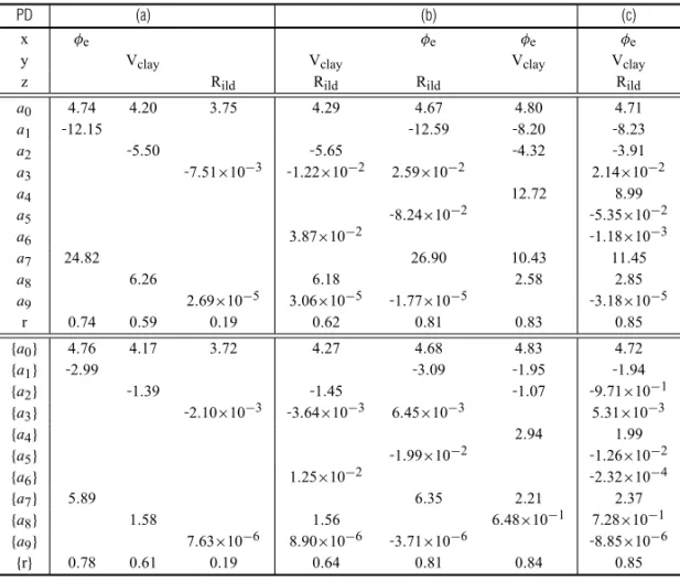
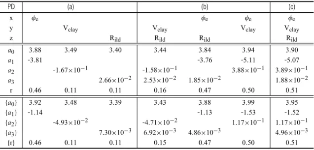
Table 1– Least-squares regression coefficients for P-wave velocity models at well-4. Two general forms are considered:vp = a0+a1x+a2y+a3zandvp=a0exp[a1x+a2y+a3z]. Fractional effective porosity (x≡φe), shaliness (y≡Vclay) and electrical resistivity (z≡Rildin Ohm.m) are the parameters of the dependence shown in the first column of the table. Each column in (a) and (b) provides six empirical models. Between braces are the coefficients associated to exponential empirical models. In order to obtain a velocity model, simply neglect one or two dependence parameters in both considered general forms. The last column in (c) provides the two empirical models having full parameter dependence. Regression coefficients have units in such a way thatvpis in km/s. The symbolrstands for correlation coefficient.
PD (a) (b) (c)
x φe φe φe φe
y Vclay Vclay Vclay Vclay
z Rild Rild Rild Rild
a0 4.27 3.92 3.72 3.97 4.29 4.42 4.43
a1 -4.00 -4.40 -3.76 -4.06
a2 -1.79 -1.84 -1.44 -1.38
a3 -3.56×10⁻³ -4.05×10⁻³ 3.30×10⁻³ 2.40×10⁻³
r 0.70 0.42 0.17 0.47 0.72 0.78 0.79
{a0} 4.26 3.87 3.69 3.93 4.28 4.43 4.44
{a1} -1.06 -1.15 -9.90×10⁻¹ -1.07
{a2} -4.60×10⁻¹ -4.70×10⁻¹ -3.60×10⁻¹ -3.50×10⁻¹
{a3} -9.88×10⁻⁴ -1.11×10⁻³ 8.16×10⁻⁴ 5.87×10⁻⁴
{r} 0.71 0.45 0.17 0.49 0.73 0.79 0.80
Table 2– Least-squares regression coefficients for P-wave velocity models at well-4, but assuming the following gene-ral forms: vp = a0+a1x+a2y+a3z+a4x y+a5x z+a6y z+a7x2+a8y2+a9z2andvp = a0exp[a1x+a2y+a3z+a4x y+a5x z+a6y z+a7x2+a8y2+a9z2]. The same observations in Table 1 concerning empirical model derivation, parameter dependence and units apply for Table 2.
PD (a) (b) (c)
x φe φe φe φe
y Vclay Vclay Vclay Vclay
z Rild Rild Rild Rild
a0 4.74 4.20 3.75 4.29 4.67 4.80 4.71
a1 -12.15 -12.59 -8.20 -8.23
a2 -5.50 -5.65 -4.32 -3.91
a3 -7.51×10⁻³ -1.22×10⁻² 2.59×10⁻² 2.14×10⁻²
a4 12.72 8.99
a5 -8.24×10⁻² -5.35×10⁻²
a6 3.87×10⁻² -1.18×10⁻³
a7 24.82 26.90 10.43 11.45
a8 6.26 6.18 2.58 2.85
a9 2.69×10⁻⁵ 3.06×10⁻⁵ -1.77×10⁻⁵ -3.18×10⁻⁵
r 0.74 0.59 0.19 0.62 0.81 0.83 0.85
{a0} 4.76 4.17 3.72 4.27 4.68 4.83 4.72
{a1} -2.99 -3.09 -1.95 -1.94
{a2} -1.39 -1.45 -1.07 -9.71×10⁻¹
{a3} -2.10×10⁻³ -3.64×10⁻³ 6.45×10⁻³ 5.31×10⁻³
{a4} 2.94 1.99
{a5} -1.99×10⁻² -1.26×10⁻²
{a6} 1.25×10⁻² -2.32×10⁻⁴
{a7} 5.89 6.35 2.21 2.37
{a8} 1.58 1.56 6.48×10⁻¹ 7.28×10⁻¹
{a9} 7.63×10⁻⁶ 8.90×10⁻⁶ -3.71×10⁻⁶ -8.85×10⁻⁶
Table 3– Least-squares regression coefficients for P-wave velocity models at well-37. Two general forms are considered: vp=a0+a1x+a2y+a3zandvp=a0exp[a1x+a2y+a3z]. The same observations in Table 1 concerning empirical model derivation, parameter dependence and units apply for Table 3.
PD (a) (b) (c)
x φe φe φe φe
y Vclay Vclay Vclay Vclay
z Rild Rild Rild Rild
a0 3.88 3.49 3.40 3.44 3.84 3.94 3.90
a1 -3.81 -3.76 -5.11 -5.07
a2 -1.67×10⁻¹ -1.58×10⁻¹ 3.88×10⁻¹ 3.89×10⁻¹
a3 2.66×10⁻² 2.53×10⁻² 1.85×10⁻² 1.88×10⁻²
r 0.46 0.11 0.11 0.16 0.47 0.50 0.51
{a0} 3.92 3.48 3.39 3.43 3.88 3.99 3.95
{a1} -1.14 -1.13 -1.53 -1.52
{a2} -4.93×10⁻² -4.71×10⁻² 1.17×10⁻¹ 1.17×10⁻¹
{a3} 7.30×10⁻³ 6.92×10⁻³ 4.86×10⁻³ 4.96×10⁻³
{r} 0.46 0.11 0.11 0.15 0.47 0.50 0.51
Table 4– Least-squares regression coefficients for P-wave velocity models at well-37, but assuming the following general forms: vp = a0+a1x+a2y+a3z+a4x y+a5x z+a6y z+a7x2+a8y2+a9z2andvp = a0exp[a1x+a2y+ a3z+a4x y+a5x z+a6y z+a7x2+a8y2+a9z2]. The same observations in Table 1 concerning empirical model derivation, parameter dependence and units apply for Table 4.
PD (a) (b) (c)
x φe φe φe φe
y Vclay Vclay Vclay Vclay
z Rild Rild Rild Rild
a0 3.84 3.53 2.92 2.93 3.53 3.86 3.80
a1 -3.07 -5.39 -4.22 -4.31
a2 -4.91×10⁻¹ -2.81×10⁻¹ 7.15×10⁻¹ 5.52×10⁻¹
a3 3.61×10⁻¹ 4.11×10⁻¹ 2.56×10⁻¹ 6.93×10⁻²
a4 -5.58 3.10
a5 5.26×10⁻¹ -6.16×10⁻¹
a6 -1.58×10⁻¹ 9.14×10⁻³
a7 -2.95 5.60 1.14 -2.40
a8 4.52×10⁻¹ 5.70×10⁻¹ 6.37×10⁻¹ -8.10×10⁻¹
a9 -3.86×10⁻² -4.08×10⁻² -3.44×10⁻² 2.27×10⁻³
r 0.46 0.13 0.53 0.56 0.65 0.51 0.47
{a0} 3.83 3.52 2.95 2.97 3.55 3.85 3.84
{a1} -7.59×10⁻¹ -1.57 -1.09 -1.26
{a2} -1.37×10⁻¹ -9.43×10⁻² 2.37×10⁻¹ 1.85×10⁻¹
{a3} 1.06×10⁻¹ 1.18×10⁻¹ 6.90×10⁻² 1.41×10⁻²
{a4} -1.92 7.63×10⁻¹
{a5} 2.02×10⁻¹ -1.37×10⁻¹
{a6} -3.76×10⁻² 2.70×10⁻³
{a7} -1.52 1.78 -1.28×10⁻¹ -1.04
{a8} 1.22×10⁻¹ 1.61×10⁻¹ 2.08×10⁻¹ -2.39×10⁻¹
{a9} -1.14×10⁻² -1.20×10⁻² -1.01×10⁻² 7.03×10⁻⁴
role in the variation of P-wave velocity, while the influence of sha-linessVclayis smaller thanφe. The assumption of resistivity as a parameter of influence in thevpvariation represents an attempt of considering fluid saturation. However, the resistivityRildexerts the smallest influence onvp variation. Note that the results in the third column of Table 4a represent an exception. We interpret these results as the footprint of the well-behaved resistivity and porosity logs at well-37. At this well, it seems that fluid content predominantly influences the velocities. A further interesting re-sult can be obtained as follows. Let us consider all 2-variable em-pirical models in whichφeandVclayare the governing parame-ters in thevpvariation. If we assumeφeandVclayas null quan-tities in these velocity models, the maximum P-wave velocity for the considered quartzoze matrix will hardly bevp =4.90km/s as seen in the third column of item (b) of all tables. Taking into account thatvp=5.94km/s is the velocity value recommended for quartz (Wyllie et al., 1958), the latter result forVclay =0.0
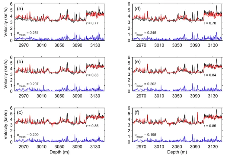
clearly indicates the influence of other different lithologies (i.e., carbonates) present in the formation. Actually, this analysis can be applied for all empirical models used in this investigation. The velocity calibration using the above-mentioned empirical models is presented in the Figures 4 and 6, including the corresponding equivalent models obtained from Eq. (6).
In Tables 2a and 4a, the magnitude of the correlation coeffici-ents shows that use of quadratic regression models improves the confidence on P-wave velocity predictions. The plots in Figures 5 and 7 exhibits velocity calibration for both wells under investi-gation, confirming the high performance of all quadratic models used. In summary, incorporation of quadratic terms into the empi-rical models decreases the misfits between measured and predic-ted velocities. As poinpredic-ted out above, the small-magnitude discre-pancies between measured and predicted velocities reveal further influence of other mixed lithologies forming the sedimentary in-terval under analysis.
2970 3010 3050 3090 3130
0 1 2 3 4 5 6 (a)
emean = 0.288
r = 0.70
V e lo ci ty (km/ s)
2970 3010 3050 3090 3130
0 1 2 3 4 5 6 (b) e
mean = 0.246
r = 0.78
V e lo ci ty (km/ s)
2970 3010 3050 3090 3130
0 1 2 3 4 5 6 (c)
emean = 0.243
r = 0.79
Depth (m) V e lo ci ty (km/ s)
2970 3010 3050 3090 3130
0 1 2 3 4 5 6 (d)
emean = 0.279
r = 0.71
2970 3010 3050 3090 3130
0 1 2 3 4 5 6 (e) e
mean = 0.238
r = 0.79
2970 3010 3050 3090 3130
0 1 2 3 4 5 6 (f)
emean = 0.235
r = 0.80
Depth (m)
2970 3010 3050 3090 3130 0 1 2 3 4 5 6 (a)
emean = 0.251
r = 0.77
V e lo ci ty (km/ s)
2970 3010 3050 3090 3130
0 1 2 3 4 5 6 (b) e
mean = 0.207
r = 0.83
V e lo ci ty (km/ s)
2970 3010 3050 3090 3130
0 1 2 3 4 5 6 (c)
emean = 0.200
r = 0.85
Depth (m) V e lo ci ty (km/ s)
2970 3010 3050 3090 3130
0 1 2 3 4 5 6 (d)
emean = 0.245
r = 0.78
2970 3010 3050 3090 3130
0 1 2 3 4 5 6 (e) e
mean = 0.202
r = 0.84
2970 3010 3050 3090 3130
0 1 2 3 4 5 6 (f)
emean = 0.195
r = 0.85
Depth (m)
Figure 5– Similarly as in Figure 4, but applying the following empirical models (see Table 2): (a)vpmod =4.74−12.15φe+24.82φe2,
(b)vpmod =4.80−8.20φe−4.32 Vclay+12.72φeVclay+10.43(φe)2 + 2.58×(Vclay)2, (c)vpmod = 4.71−8.23φe−
3.91 Vclay+2.14×10⁻²Rild+8.99φeVclay−5.35×10⁻²φeRild−1.18×10⁻³VclayRild+11.45(φe)2+2.85(Vclay)2−
3.18×10⁻⁵(Rild)2, (d)vpmod=4.76 exp[−2.99φe+5.89(φe)2], (e)vpmod=4.83 exp[−1.95φe−1.07 Vclay+2.94φeVclay+ 2.21(φe)2+6.48×10⁻¹(Vclay)2], (f)vpmod = 4.72 exp[−1.94φe−9.71×10⁻¹Vclay+5.31×10⁻³Rild+1.99φeVclay−
1.26×10⁻²φeRild−2.32×10⁻⁴VclayRild+2.37(φe)2+7.28×10⁻¹(Vclay)2−8.85×10⁻⁶(Rild)2].
In the following, we use some empirical models in order to perform comparison with the model derived by Han et al. (1986) for brine-saturated sandstone cores at 20 MPa:vpmod= 5.49−6.94φe −2.17 Vclay. Although derived from satura-ted rock samples, this empirical model ignores fluid saturation as a parameter of velocity dependence. In Figure 8 we perform comparison using empirical models derived only from the general form in Eq. (5), for the correlation coefficients in Tables 1-4 show equivalence with the regression models obtained from Eq. (6). However, we use models in which effective porosityφe, shaliness Vclayand resistivityRilddescribe P-wave velocity dependence. In Figure 8, thicker black curves denote measured velocities con-verted from corresponding P-wave sonic logs.
Let us consider well-4. In Figure 8a, we plot the empirical mo-del forvpwhich can be constructed with regression coefficients in item (c) of Table 1; Figure 8b shows thevpplot using the model with the regression coefficients in item (c) of Table 2. The calibra-tion applying these regression models shows good prediccalibra-tions
of P-wave velocities in the sandstone intervals of well-4. Abso-lute deviations are small throughout the mixed lithologies, confir-ming the robustness of the 3-variable empirical models for velo-city description. The regression model of Han et al. (1986) shows large misfits in the sealing intervals of well-4 because it was derived using data from brine-saturated sandstones at 20 MPa. Thus, we can infer that the sandstone intervals at this well are submitted to an effective pressure of 20 MPa.
2970 3010 3050 3090 3130 0 1 2 3 4 5 6 e
mean = 0.135
r = 0.46 (a) V e lo ci ty (km/ s)
2970 3010 3050 3090 3130
0 1 2 3 4 5 6
emean = 0.129
r = 0.50 (b) V e lo ci ty (km/ s)
2970 3010 3050 3090 3130
0 1 2 3 4 5 6 e
mean = 0.127
r = 0.51 (c) Depth (m) V e lo ci ty (km/ s)
2970 3010 3050 3090 3130
0 1 2 3 4 5 6 e
mean = 0.136
r = 0.46 (d)
2970 3010 3050 3090 3130
0 1 2 3 4 5 6
emean = 0.130
r = 0.50 (e)
2970 3010 3050 3090 3130
0 1 2 3 4 5 6 e
mean = 0.128
r = 0.51 (f)
Depth (m)
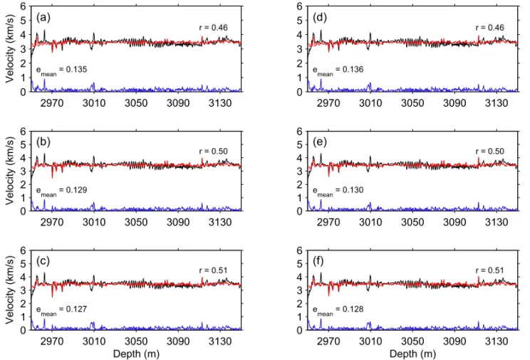
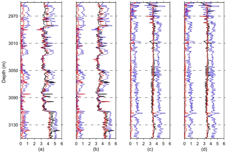
Figure 6– Application of regression models for P-wave velocity predictionvpmodat well-37. Black curve denotes P-wave velocityvpmeas converted from measured sonic log. In accordance with the regression coefficients in Table 3, the empirical models (red curves) are: (a)vpmod= 3.88−3.81φe, (b)vpmod=3.94−5.11φe+3.88×10⁻¹Vclay, (c)vpmod=3.90−5.07φe+3.89×10⁻¹Vclay+1.88×10⁻²Rild,
(d)vpmod = 3.92 exp[−1.14φe], (e)vpmod = 3.99 exp[−1.53φe+1.17×10⁻¹Vclay], (f)vpmod = 3.95 exp[−1.52φe+
1.17×10⁻¹Vclay+4.96×10⁻³Rild]. Blue curves represent absolute residuals between measured and predicted velocity logs. Each plot correspondingly shows the mean absolute residualemeanand the correlation coefficientr.
CONCLUSIONS
Use of regression analysis represents a very suitable procedure for establishing velocity dependence in mixed lithologies. Although most published works show core plug measurements as the main source of information, rock physical properties extracted from well log data can also be used in establishing a P-wave regression model. The importance of porosity and shaliness in describing velocity variation represents the primary choice for these parame-ters as the variables of the dependence. Considering resistivity as a further velocity dependence parameter may represent a refi-nement of the empirical model, since it can indirectly incorporate fluid-saturation effects into the velocity variation.
Additional conclusions can be drawn from the correlation co-efficients in Tables 4. The results presented therein with 1-variable empirical models clearly exhibit the need for more in-formation on the rock properties. For porosity as the main de-pendence variable, P-wave velocity can be described better than
using only shaliness or electrical resistivity. If porosity and sha-liness are included in the empirical model for describing the ve-locity variation, the correlation coefficients increase significantly. Further incorporation of electrical resistivity as a parameter of the velocity dependence produces higher correlation coefficients. In this case, the increase in correlation coefficients is far higher for quadratic empirical models. These conclusions apply for both general forms in Eqs. (5) and (6), from which we obtained the empirical models used in the present paper.
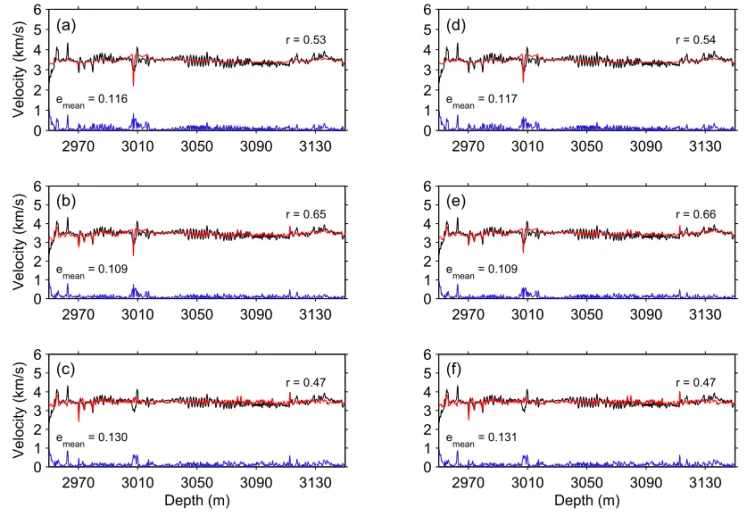
2970 3010 3050 3090 3130 0 1 2 3 4 5 6 e
mean = 0.116
r = 0.53 (a) V e lo ci ty (km/ s)
2970 3010 3050 3090 3130
0 1 2 3 4 5 6 e
mean = 0.109
r = 0.65 (b) V e lo ci ty (km/ s)
2970 3010 3050 3090 3130
0 1 2 3 4 5 6 e
mean = 0.130
r = 0.47 (c) Depth (m) V e lo ci ty (km/ s)
2970 3010 3050 3090 3130
0 1 2 3 4 5 6 e
mean = 0.117
r = 0.54 (d)
2970 3010 3050 3090 3130
0 1 2 3 4 5 6 e
mean = 0.109
r = 0.66 (e)
2970 3010 3050 3090 3130
0 1 2 3 4 5 6 e
mean = 0.131
r = 0.47 (f)
Depth (m)
Figure 7– Similarly as in Figure 6, but applying the following empirical models (see Table 4): (a)vpmod = 2.92+3.61×10⁻¹Rild− 3.86×10⁻²(Rild)2, (b)vpmod=3.53−5.39φe+2.56×10⁻¹Rild+5.26×10⁻¹φe×Rild+5.60(φe)2−3.44×10⁻²(Rild)2, (c) vpmod=3.80−4.31φe+5.52×10⁻¹Vclay+6.93×10⁻²Rild+3.10φeVclay−6.16×10⁻¹φeRild+9.14×10⁻³VclayRild− 2.40(φe)2−8.10×10⁻¹(Vclay)2+2.27×10⁻³×(Rild)2, (d)vpmod = 2.95 exp[1.06×10⁻¹Rild−1.14×10⁻²(Rild)2], (e)
vpmod = 3.55 exp[ −1.57φe+6.90×10⁻²Rild+2.02×10⁻¹φeRild +1.78(φe)2− 1.01×10⁻²(Rild)2], (f)vpmod =
3.84 exp[ −1.26φe+1.85×10⁻¹Vclay+1.41×10⁻²Rild+7.63×10⁻¹φeVclay−1.37×10⁻¹φeRild+2.70×10⁻³Vclay
Rild−1.04(φe)2−2.39×10⁻¹(Vclay)2+7.03×10⁻⁴(Rild)2].
resistivity log. Assumption of ln(Rild)smooths such outliers, giving to better velocity correlations.
ACKNOWLEDGMENTS
This paper shows results of the research project “Caracterizac¸˜ao de Anisotropia S´ısmica Usando Perfis Geof´ısicos de Poc¸os de Petr´oleo e G´as”, which has support from The National Council for Scientific and Technological Development, CNPq/Brazil (proc. no. 471647/2006-3). Preliminary results of this paper were presented at the 10thInternational Congress of the Brazilian Geophysical Society (SBGf), at the Rio Oil & Gas 2008 Expo and Conference and at the III Symposium of SBGf. Fabr´ıcio Augusto acknowledges a research scholarship from CAPES/Brazil for the development of his master dissertation in Geophysics at Obser-vat´orio Nacional, Brazil. We sincerely appreciate the contributi-ons of an anonymous reviewer.
REFERENCES
ARCHIE GE. 1950. Introduction to petrophysics of reservoir rocks. Bul-letin of the American Association of Petroleum Geologists, 34: 943–961.
CASTAGNA JP, BATZLE ML & EASTWOOD RL. 1985. Relationships between compressional-wave and shear-wave velocities in clastic silicate rocks. Geophysics, 50: 571–581.
CASTAGNA JP, BATZLE ML & KAN TK. 1993. Rock physics: The link between rock properties and AVO response. In: CASTAGNA JP & BAC-KUS MM (Eds.). Offset-dependent reflectivity – Theory and practice of AVO analysis. Investigations in Geophysics no. 8, Society of Exploration Geophysicists, OK, 135–171.
DEWAN JT. 1983. Essentials of modern open-hole log interpretation. PennWell Books, 361 pp.
0 1 2 3 4 5 6 2970
3010
3050
3090
3130
(a)
D
e
p
th
(m)
0 1 2 3 4 5 6
(b)
0 1 2 3 4 5 6
(c)
0 1 2 3 4 5 6
(d)
Figure 8– Comparison of regression models for P-wave velocity prediction. The comparison is performed using the empirical relation in Han et al. (1986) for rock plugs submitted to an effective pressure of 20 MPa: vpmod = 5.49−6.94φe−2.17 Vclay(blue curve). At well-4 (red curves): (a)vpmod = 4.43− 4.06φe−1.38 Vclay +2.40×10⁻³Rild, and (b)vpmod = 4.71− 8.23φe−
3.91 Vclay+2.14×10⁻²Rild+8.99φeVclay−5.35×10⁻²φeRild−1.18×10⁻³VclayRild+11.45(φe)2+2.85(Vclay)2−
3.18×10⁻⁵(Rild)2. At well-37 (red curves): (c)vpmod =3.90−5.07φe+3.89×10⁻¹Vclay+1.88×10⁻²Rild, and (d)vpmod=
3.80−4.31φe+5.52×10⁻¹Vclay+6.93×10⁻²Rild+3.10φeVclay−6.16×10⁻¹φeRild+9.14×10⁻³VclayRild−2.40(φe)2−
8.10×10⁻¹(Vclay)2+2.27×10⁻³(Rild)2. Absolute residuals (left curves in the plots) have the same color as the corresponding empirical model. Units in km/s.
DOMENICO SN. 1976. Effect of brine-gas mixture on velocity in an un-consolidated sand reservoir. Geophysics, 41: 882-894.
EBERHART-PHILLIPS D, HAN D-H & ZOBACK MD. 1989. Empirical re-lationships among seismic velocity, effective pressure, porosity, and clay content in sandstone. Geophysics, 54: 82–89.
ELLIS DV. 1987. Well logging for Earth scientists. Elsevier Science Publishing Co. Inc., 550 pp.
FAUST LY. 1951. Seismic velocity as a function of depth and geologic time. Geophysics, 16: 192–206.
FAUST LY. 1953. A velocity function including lithologic variation. Geo-physics, 18: 271–288.
HAN D-H, NUR A & MORGAN D. 1986. Effects of porosity and clay con-tent on wave velocities in sandstones. Geophysics, 51: 2093–2107.
KAUFMAN H. 1953. Velocity functions in seismic prospecting. Geophys-ics, 18: 289–297.
KLIMENTOS T. 1991. The effects of porosity-permeability-clay content on velocity of compressional waves. Geophysics, 56: 1930–1939.
KRIEF M, GARAT J, STELLINGWERFF J & VENTRE J. 1990. A petrophy-sical interpretation using the velocities of P and S waves (Full-waveform sonic). The Log Analyst, 31: 355–369.
LARIONOV WW. 1969. Borehole Radiometry. Nedra, Moscow. (In Rus-sian). 127 pp.
LINES LR & TREITEL S. 1984. A review of least-squares inversion and its application to geophysical problems. Geophysical Prospecting, 32: 159–186.
MILLER SLM & STEWART RR. 1990. Effects of lithology, porosity and shaliness on P- and S-wave velocities from sonic logs. Canadian Journal of Exploration Geophysics, 26: 94–103.
OLIVEIRA JK & MARTINS JL. 2003. Efeitos da porosidade e argilosi-dade nas velociargilosi-dades de ondas compressionais no arenito Namorado, Bacia de Campos, Brasil. In: 8thIntern. Cong. of the Brazilian Geophys. Society, 14-18 September, Hotel Intercontinental, Rio de Janeiro, Brazil, CD-ROM. (In Portuguese).
PENNINGTON WD. 2001. Reservoir geophysics. Geophysics, 66: 25–30.
RAYMER DS, HUNT ER & GARDNER JS. 1980. An improved sonic tran-sit time-to-porotran-sity transform. In: 21stAnnual Meeting of the Society of
Professional Well Log Analysts, paper P.
TIGRE CA & LUCCHESI CF. 1986. Estado atual do desenvolvimento da Bacia de Campos e perspectivas. In: Semin´ario de Geologia de Desen-volvimento e Reservat´orio, DEPEX-PETROBRAS, Rio de Janeiro, 1-12. (In Portuguese).
TOSAYA C & NUR A. 1982. Effects of diagenesis and clays on compres-sional velocities in rocks. Geophysical Research Letters, 9: 5–8.
TOKS ¨OZ MN, CHENG CH & TIMUR A. 1976. Velocities of seismic waves in porous rocks. Geophysics, 41: 621–645.
WATT JP, DAVIES GF & O’CONNELL RJ. 1976. The elastic properties of composite materials. Rev. Geophys. and Space Physics, 14: 541–563.
WYLLIE MRJ, GREGORY AR & GARDNER LW. 1956. Elastic wave velo-cities in heterogeneous and porous media. Geophysics, 21: 41–70.
WYLLIE MRJ, GREGORY AR & GARDNER LW. 1958. An experimental investigation of factors affecting elastic wave velocities in porous media. Geophysics, 23: 459–493.
XU S & WHITE RE. 1995. A new velocity model for clay-sand mixtures. Geophysical Prospecting, 43: 91–118.
NOTES ABOUT THE AUTHORS
Fabr´ıcio de Oliveira Alves Augustoholds a BS degree (2006) in physics from Fluminense Federal University, Brazil. He earned his master dissertation (February 13th, 2009) in the post-graduation course in geophysics at Observat´orio Nacional, Ministry of Science and Technology, Brazil. He is a member of SBGf.