www.scielo.br/rbg
INFLUENCE OF SEA WATER RESISTIVITY ON MCSEM DATA
Edelson da Cruz Luz and C´ıcero Roberto Teixeira R´egis
Recebido em 15 junho, 2009 / Aceito em 17 setembro, 2009 Received on June 15, 2009 / Accepted on September 17, 2009
ABSTRACT.The Marine Controlled Source ElectroMagnetic (MCSEM) method is a geophysical tool for the detection of resistive targets in the subsurface of the oceanic floor. In this work we model MCSEM data in one-dimensional environments, including variations in the resistivity of the ocean water, as horizontal layers of uniform resistivity. Such variations can arise from the influence of marine currents, temperature gradients or any other source of influence on the water salinity. We study the effect of such variations on the MCSEM data. Our results show that the interpretation can be strongly influenced, especially for normalized data. We see that changes in the water resistivity have a similar effect on the data as changes in the water depth, and that both affect the attenuation of the so called “air-wave”.
Keywords: MCSEM, modeling, sea water resistivity.
RESUMO.O Marine Controlled Source ElectroMagnetic (MCSEM) ´e um m´etodo geof´ısico para a detecc¸˜ao de camadas resistivas contidas abaixo do assoalho oceˆanico. Neste trabalho n´os modelamos os dados do MCSEM em um ambiente unidimensional, incluindo variac¸˜oes na resistividade da ´agua do mar, na forma de camadas de resistividades uniformes. Estas variac¸˜oes na resistividade da ´agua podem surgir devido `a influˆencia de correntes marinhas, gradientes de temperatura ou mudanc¸a na salinidade da ´agua. N´os estudamos o efeito destas variac¸˜oes nos dados do m´etodo MCSEM. Nossos resultados mostram que a interpretac¸˜ao pode ser fortemente influenciada, principalmente quando s˜ao analisados os dados normalizados. Vimos que as mudanc¸as na resistividade da ´agua tˆem um efeito sobre os dados similar `aquele de mudanc¸as na profundidade da lˆamina d’´agua, sendo que ambos influenciam na atenuac¸˜ao da chamada “air-wave”.
Palavras-chave: MCSEM, modelagem, resistividade da ´agua do mar.
INTRODUCTION
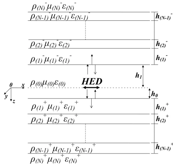
The Marine Controlled Source Electromagnetic method has gai-ned importance to the oil and gas industry for the possibility of detecting hydrocarbons directly in the sea bed under deep wa-ters. The method has been used to detect resistive targets in the conductive environment under the sea. In a typical MCSEM sur-vey, an electric dipole is towed near the sea bed, over an array of receivers placed on the sea floor. This transmitter generates a signal that travels through the water and penetrates the rock formations, where it is partly reflected by the interfaces between regions of different resistivities (Fig. 1). The receivers measure reflected signal, together with the field coming directly from the source plus the field reflected on the air-water interface. The me-asured electric field amplitudes and phases are affected by the presence of resistive structures, such as a salt intrusion, carbo-nates, volcanics, and reservoir rocks filled with oil or gas.
As the field propagates through the sea water, it can be sig-nificantly affected by changes in the resistivity, which is funda-mentally determined by salinity and temperature of the water. The relationship between the resistivity, salinity and temperature is complicated. The temperature near the surface of the sea can be very different from that at the bottom. The higher the tempera-ture, the higher is the rate of evaporation on the surface, which can affect the salinity. Temperature also increases the saturation point of the salt solution, which means that warmer water can hold more dissolved salt then cold water. Higher salinity means a greater number of charge carriers (ions) in the solution, which causes resistivity to decrease. Temperature also affects the mobi-lity of the charge carriers (ions) in the solution. Increase in tem-perature causes the ion mobility to rise, which also brings the resistivity down.
In previous works, the ocean has always been modeled as a uniform layer, with resistivity around 0.3m. Possible vari-ations in the water resistivity due to non uniformity in salinity and temperature are mentioned by Constable & Srnka (2007), however we find no model for those variations in the literature of the method.
In this work we simulate MCSEM data in 1D environments with the ocean water modeled as a sequence of uniform horizon-tal layers.
The measured electromagnetic field is strongly influenced by the propagation through the ocean water. Our results show how even that narrow range of variation in the water resistivity is enough to alter the data sufficiently to influence their interpreta-tion, by changing its attenuation of the field in the water.
1D MODELING
The sea water is usually described as a homogeneous layer with a 0.3m resistivity (Chave et al., 1991; Eidesmo et al., 2002; Constable & Weiss, 2006). However, variations in the sea wa-ter resistivity are always present in a greawa-ter o lesser extent. As a simple first approximation to assess the extent of that ef-fect, we model the ocean as a sequence of homogeneous layers with different resistivities. Was chosen the resistivity model in the PANGEA data bank (Schulz, 2001) which better represent the Brazilian sea.
To calculate the fields we model the source as a Dirac delta function located in the deepest water layer. We follow the method described in Nabighian (1991), with the reflection coefficients sui-tably altered in order to include the reflections on the interfaces above the dipole source.
One fundamental feature of the propagation of the electro-magnetic field is the attenuation by its interaction with the con-ductive medium due to the conversion of electromagnetic energy into heat. The attenuation is described by the parameter known as the skin depth (δ), which is defined as the distance after which the plane wave field is attenuated by a factor 1/e, ebeing the base of the natural logarithms. For a homogeneous, non magnetic medium, the skin depth is approximated by
δ=503.29
rρ
f (1)
whereρis the electrical resistivity of the medium and f is the frequency of the field.
When we allow the resistivity to vary, we are in fact chan-ging the skin depth, or the attenuation of the fields propagating through the water. We interpret our results in the light of those changes in the rates of attenuation.
RESULTS
We present curves for the magnitude and phase of the fields as functions of the source-receiver offset. When we measure the electric field in the same direction as the dipole moment we have the in-line (field purely radial) array and when we measure the fields in a direction perpendicular to the dipole moment we have the broadside (field purely azimuthal) array. The curves for those arrays have different characteristics as they measure diffe-rent components of the fields.
homogene-y
h
0h
1(0) (0) (0)
(1)
+
(1)
+
(1)
+
0
x
z
HED
(1)
-
(1)
-
(1)
-(2)
-
(2)
-
(2)
-(N-1)
-
(N-1)
-
(N-1)
-(2)
+
(2)
+
(2)
+
(N-1)
+
(N-1)
+
(N-1)
+
h
(1)-h
(2)-h
(1)+h
(2)+h
(N-1)+h
(N-1)-(N)
-
(N)
-
(N)
-(N)
+
(N)
+
(N)
+
Figure 1– Model with the non homogeneous water layer.
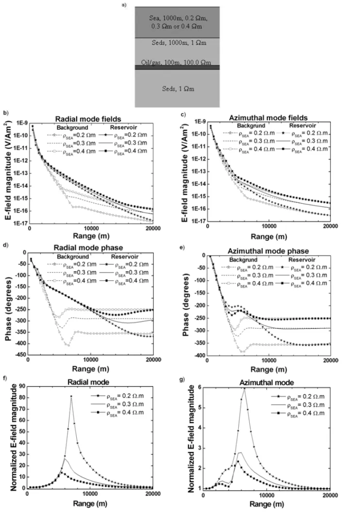
ous medium into which may be superimposed a resistive layer 100m thick and 100.m, at a depth of 1,000m from the sea floor. Energizing this canonical model we will have a source located 50m above the sea floor, with a frequency of 0.5Hz.
The effect of resistive targets on the field values is subtle in the MCSEM method. In order to make that effect more apparent it is customary to show the field magnitudes normalized by the data from a reference receiver, which supposedly is in a posi-tion where there is no influence of the resistive target (Røsten et al., 2003; Johnstad et al., 2005; Maaø et al., 2007). In theoreti-cal studies this normalization is made with field values theoreti-calculated for a model with a homogeneous earth.
For small off-sets, the receivers register mainly the direct field from the source, which does not depend on the rock layers. The influence of the resistive targets is relatively stronger in in-termediate off-sets and farther away from the source the do-minant effect is from the so called air-wave, which is gene-rated in the air-water interface and is the same regardless of the resistivities in the rocks bellow. In this way, the normali-zed curves show peaks whose position and intensity depend on
the relative influence of the fields arriving in the receivers from the water and from the sea floor.
In an exercise to show the limits of the variations of the fi-elds due to the water resistivity we show the results for a mo-del with a homogeneous water layer with three different resistivity values: 0.2.m, 0.3.m and 0.4.m. Those values will be used in our next models.
Figure 2 shows the results for these first models. As the water resistivity falls, the attenuation of the field in the water becomes stronger, which means that the skin depth gets smaller. The re-lative influence of the rock layers on the measured data is then increased and the air-wave starts to dominate the response in a position farther from the source. These effects appear clearly in the phase curves, and also in the position of the peaks of the normalized curves.
If the water resistivity is higher the opposite effects are ob-served: the influence of the rock layers is less strong and the peaks in the normalized curves are lower and closer to the source position.
The ocean water can be more conductive than the 0.3.m of the canonical model if the surface temperatures are high enough, as is the case in low latitude areas. The PANGEA data bank (Schulz, 2001) gives us a resistivity profile of 0.174.m near the surface with a temperature of 27.77◦C and 0.303.m
at the bottom with 4.60◦C, at a latitude: 2.2050, at a longitude:
–35.1817.
Our model with a non homogeneous ocean is shown in Fig. 3. As we build this model with lower resistivities, the fi-elds from the air-water interface are more attenuated and the resistive layer has a stronger effect on the data than in the case of the homogeneous 0.3.m sea. Accordingly, the anomaly in the normalized curve is increased, as we can observe in Figure 3-f,g. Also notice the shift in the peak anomaly, showing that the air-wave starts to dominate the curve farther from the source than in the case of the homogeneous sea.
Other parameters that alter the relative effect of the air-wave are the frequency and the water depth. One interesting point is that variations in the ocean depth affect the curves in a similar way as the variations in the water resistivity whereas frequency variation shows quite a different outcome.
The deeper the water, the less influence is felt from the air-wave and its dominance starts farther from the transmitter, so the anomaly peak in the normalized curves are shifted to the right in our graphs, as shown in Figure 4-a,b. Notice that in shallow wa-ters, the anomaly peaks are lower, as was the case with the more resistive water. We interpret this by the same reasoning: the fi-elds that arrive in the receiver through the water suffer a greater attenuation when the ocean is deeper as well as when it is more conductive, which makes the relative influence of the sea floor stronger in those cases.
Another way to decrease the skin depth is to raise the fre-quency. Now, when we observe the curves for a homogene-ous sea with three frequencies (Fig. 4-c,d) we see that increa-sing the frequency increases the anomaly peaks in the normalized curves but it also shifts the peaks toward the source, a behavior we would expect as a result of decreasing the skin depth of the field in the water, except that now, by changing frequency, we af-fect the field in the sea floor as well as in the water. The relative effect of increasing the frequency is, then, stronger in the field th-rough the water, since the difference between the skin depths in the water and in the sea floor is smaller the higher the frequency.
The combined effect makes the air-wave dominate the method’s response sooner in higher than in lower frequencies.
CONCLUSION
The interpretation of MCSEM data is a difficult task, the signatures of the targets are often hard to assess. The resistivity structure of the ocean water is a factor that should not be overlooked, since it can affect the data in subtle ways. Even relatively small variations on the ocean water conductivity can alter the data.
We have shown that increasing the water conductivity has a similar effect as increasing the ocean depth, since in both cases the fields traveling through the water are more strongly attenua-ted when they arrive in the receivers. In a more conductive wa-ter, the target layer response is enhanced in the measured sig-nal, so that its associated anomaly tends to be higher than that in a less conductive water.
It is common practice to measure the resistivity profile of the ocean when surveying, so that information is readily available and should always be part of the interpretation process.
When one needs to model MCSEM data to help in the analy-sis and interpretation one should always include the true reanaly-sisti- resisti-vity profile of the water in the models, so that any normalization results in reliable data.
Our next step in this research will be to perform inversion in data from 1D and 2D environments. Those are tasks where it will be critical to work with the correct water resistivity varia-tion. The use of a uniform water column in an interpretative mo-del will lead to solutions that are far from the correct geoelectric structures that generates the data.
ACKNOWLEDGMENTS
This work was suggested by Prof. Luiz Rijo. We thank the UFPA/ANP-PRH-06 for the scholarship which partially financed this work. Thanks also to Victor Souza and Marcos Welby, for the rich discussions and suggestions that have been very helpful to this ongoing research.
REFERENCES
CHAVE AD, CONSTABLE SC & EDWARDS RN. 1991. Electrical explora-tion methods for the seafloor. In: NABIGHIAN MN (Ed.). Electromagnetic Methods in Applied Geophysics, 2: SEG, 931–966.
CONSTABLE SC & SRNKA LJ. 2007. An introduction to marine controlled-source electromagnetic methods for hydrocarbon exploration. Geophysics, 72(2) (March-April 2007); P. WA3-WA12, 6 Figs.
Figure 4– Results from the model with the different deep water layers and different frequencies; (a,c) Electric field magnitude for the Radial mode; (b,d) Normali-zed field in the Radial mode.
hydrocarbons with marine EM methods: Insights from 1D modeling. Geophysics, 71(2) (March-April 2006); P. G43-G51, 11 Figs., 1 Table.
EIDESMO T, ELLINGSRUD S, MacGREGOR LM, CONSTABLE SC, SINHA MC, JOHANSEN S, KONG FN & WESTERDAHL H. 2002. Sea Bed Log-ging (SBL), a new method for remote and direct identification of hydro-carbon filled layers in deepwater areas. News feature, 20(3): 144–152.
JOHNSTAD SE, FARRELLY BA & RINGSTAD C. 2005. EM seabed log-ging on the Troll Field. 67thEAGE Conference & Exhibition, Extended Abstracts, H010.
MAAØ FA, JOHNSTAD SE, GABRIELSEN PT & PANZNER M. 2007. Azimuth Decomposition of SBL Data. EGM International Workshop
In-novation in EM, Grav and Mag Methods: a new Perspective for Explora-tion. Italy. 4 pp.
NABIGHIAN MN (Ed.). 1991. Electromagnetic Methods in Applied Geophysics, Vol. 2, Application, Parts A and B, Society of Exploration Geophysicists, Chapt. 12, 931–940.
RØSTEN T, JOHNSTAD SE, ELLINGSRUD S, AMUNDSEN HEF, JOHAN-SEN S & BREVIK I. 2003. A Sea Bed Logging (SBL) calibration survey over the Ormen Lange gas field. 65thEAGE Conference & Exhibition, Extended Abstracts, P058.
NOTES ABOUT THE AUTHORS
Edelson da Cruz Luzreceived his L.Sc. in Physics at the Universidade Federal do UFPA (2004), his M.Sc. in Geophysics at the Universidade Federal do Par´a-UFPA (2007). Currently, he is carrying on his D.Sc. at the Universidade Federal do Par´a-Par´a-UFPA focussing on modeling and inversion of MMT (Marine Magnetotelluric) and MCSEM (Marine Controlled Source ElectroMagnetic) using parallel computing.