The dynamic intensity of CO
2emissions:
empirical evidence for the 20
thcentury
A intensidade dinâmica das emissões de CO
2:
evidências empíricas para o século XX
DIEGO CARNEIRO
GUILHERME IRFFI*
RESUMO: A relação entre crescimento econômico e degradação ambiental (poluição) tem sido amplamente investigada por acadêmicos, principalmente, em virtude da constatação de que fatores antrópicos podem inluir no clima global. O mecanismo pelo qual isso acon-tece, o dito efeito estufa, está diretamente relacionado ao acúmulo de certos gases na at-mosfera, sendo o principal deles o dióxido de carbono, oriundos da atividade produtiva. Assim, o presente trabalho pretende estimar a taxa a qual a intensidade de emissão, razão
entre o nível de emissões de CO2 e o PIB, vem crescendo desde o início do século XX para
um grupo de 24 países. Os resultados mostraram que Inglaterra e Estados Unidos possuem tendência negativa da intensidade de emissão, ao contrário do que foi observado para a Índia. Testou-se também a presença de mudanças estruturais, que se mostraram presentes coincidindo com a Primeira Guerra Mundial (1914 a 1918), a Grande Depressão dos anos 1930 e os Choques do Petróleo da década de 1970. A partir das análises dos resultados,
pode-se dizer que os países desenvolvidos são menos intensivos em emissão, ou seja, é evi-dente o papel da tecnologia como instrumento de redução da intensidade de emissão global.
PALAVRAS-CHAVE: Intensidade de emissão; dióxido de carbono; aquecimento global.
ABSTRACT: The debate around the economic growth and environmental degradation is the hot topic among academics. However, up to a point, all of them embrace the uncontro-versial view that tells us that anthropic factors have leverage on global climate. It happens
that the so-called greenhouse effect is closely related to the accumulation of certain gases in
the atmosphere, e.g., carbon dioxide, whose original source comes from productive sectors. Thus, our purpose in this article is to estimate the rate of emission intensity – here we mean
the ratio between CO2 emissions and GDP – which has increased since the early part of the
20th century. To support that idea, this study reports on data from 24 different countries. In
terms of C02 emission, the results undoubtedly show that United Kingdom and the United
* Doutorando em Economia pelo CAEN/UFC – Universidade Federal do Ceará. E-mail: dr.carn@gmail. com; Professor do Departamento de Economia Aplicada e do CAEN/UFC. E-mail: [email protected]. Submitted: 2/March/2015; Approved: 5/October/2016.
Brazilian Journal of Political Economy, vol. 37, nº 4 (149), pp. 772-788, October-December/2017
773
Revista de Economia Política 37 (4), 2017 • pp. 772-788
States highlight a negative picture, particularly when both are compared to India. It should be noted the presence of structural changes, which coincide with three major historical events: the world war I (1914-1918), the Great Depression in the 1930s, and inally the Oil-price shocks in the 1970s. As the result of the analysis demonstrates, the amount of emission produced by developing countries is surprisingly low. That the technology reveals its relative merit for reducing the overall emission intensity is transparently obvious.
KEywORDS: Emission intensity; carbon dioxide; global warming. Jel Classification: K32.
INTRODUCTION
Even if the projections could all be mistaken, it has been a hardly deeply dis-turbing fact that economic externalities cause problems for the environment. Giv-en that climate change is directly and necessarily influGiv-enced by human affairs, cli-mate researchers have been concerned about the predicted bad effects of clicli-mate change without sacrificing the prosperity on the part of presently existing people. All this can be recognized but the tricky point is how one may properly produce while minimize environmental impact.
In fact, in the early 21st century empirical data were presented by the Intergov-ernmental Panel on Climate Change (2000, 2001, 2003). Examinations pointed out with increasing knowledge of the global temperature that CO2 emissions are quite significantly.
Despite the current gain visibility, that issue was early on discussed by D’Arge in the 1970s. He primarily started by taking a Malthusian scenario, bolstered by the relationship between growth in population and environmental concern and came to the conclusion that population growth, material flows, etc. produce large amounts of pollution, deteriorating progressively the natural resources. This would be, of course, in the long run unacceptable. In practical terms, what is astonishing is that the exceeding of CO2 emission occurs regarding one is stuck with the inevi-table use of energy, as an indispensable input for the production – principal sourc-es of energy are directly related to the burning of fossil fuels, having CO2 emission as a by-product. Despite existing natural resources less damageable, coal and oil have been altogether the most familiar ones, at least since the second industrial revolution (Mauro, 1973).
A matter of ongoing concern is the extent to which CO2 emission can or should affect, on grounds of efficiency, the production to a given economy. To make things simpler, an indicator that allows us to compare the efficiency between distinct economies will be required, one disposed by the ratios of CO2 emission/GDP here called emission intensity (henceforth EI).
774 Brazilian Journal of Political Economy 37 (4), 2017 • pp. 772-788
extension of other views1. Granted this well-established framework comes to com-plement them, we still need to supply two congenial findings provided by Perron and yabu (2009a, 2009b): the first estimates deterministic point placed in a context in which the signal-to-noise component can be integrated or stationary; the second admits equal properties of error, but is further dedicated to test the existence of structural change in the growth rate of EI.
The novelty here that reinforces the value of the contribution to the field is considerable: not only because this approach is clearly “econometric” compara-tively to what we have done somewhere2, rather, our enquiry into the logic of EI, namely, carried out with a bearing on its historic-serial principles, will be capable of generalization over a domain extending from 1901 to 2010, and this should in turn move us a long way toward establishing meaningful benchmarks in the field of environmental economics.
Using long-run data is by the way very useful in exploring if technological progress – which is generally meant to have a positive contribution to the GDP –, can somehow afford a reduction of CO2. Based on the results, we evaluate if growth rate in EI is positive, negative or constant over the base period, and if we can ges-ture policy implications paying attention to the effects of greenhouse gases concen-tration, similarly tending to tackle the effects of climate change.
The rest of this paper is structured as follows. Second section will describe the database, e.g., source and temporal dimension, as well as the descriptive analysis of the time series. Third section presents the strategy of estimating the growth rate in CO2 emission, that is to say, the alleged view engendered by Perron and yabu (2009a, 2009b). The analysis and further discussion of the results make up fourth section, followed by a few final commentaries.
METHOD AND DATA
C02 emission – the source
The key to providing the intended calculation for EI (encompassing 24 developed countries 1901-2010 and equivalent amount of one thousand metric ton of carbon dioxide) resides in the ratio between CO2 emission and GDP. In turn, as for the former, we make use of its data officially published by the Carbon Dioxide Information Center (CDIAC) but whose elaboration is due to Boden, Marland and Andres (2011). Such emissions come primarily from various resources, though the authors take into account the burning of fossil fuels, cement manufacture and flue gas. Additionally, as
1 we are referring to the works of Nielsson (1993), Goldemberg (1996), Mielnik and Goldemberg
(1999), Ang (1999), Roca and Alcántara (2001). The authors rely their views on visual inspection and descriptive statistics.
775
Revista de Economia Política 37 (4), 2017 • pp. 772-788
for the latter, we take data, with respect per capita GDP (for 1990 and estimated in 1990 international dollar) and population, engendered by Bolt and Zanden (2013)
from the Maddison Project.
Be they rich, developed or developing, the choice of the following countries was determined by availability and access of data sets. They are: Europe – Austria, Belgium, Denmark, Finland, France, Greece, The Netherlands, Italy, Norway, Swe-den, Switzerland, United Kingdom, Portugal and Spain; Oceania – Australia and New Zealand; North America – Canada and the United States; Latin America – Argentina, Brazil, Chile, Mexico, Peru; Asia – India.
Box 1: Variables description
Variable Description Measured
value Source
Pc GDP Per capita GDP 1990 dollars Madisson
Project
Local
residents Local residentes 1.000 people
Madisson Project
GDP Gross domestic product
[Per capita GDP vs. Local residents] 1990 dollars Calculated
CO2 Emission of carbon dioxide
1.000 metric
ton of CO2
CDIAC
Intensity Pollution originated for each dollar/a
unit of wealth [(CO2/GDP) x 1.000]
Kg. of CO2
per 1990 dollars Calculated
Source: Elaborated by the authors themselves.
Descriptive Analysis of Results
Having presented the variables, now we are ipso facto concerned with the behavior of the series along the base period. As for CO2 emission and GDP, Graphs 1 and 2 indicate, in an aggregated way, the time evolution, namely, the sum of both variables bearing in mind the aforementioned 24 countries. Graph 3 highlights evolution of the global average of EI. Going a step further, we supply the analysis by pointing out the countries and the related chiefs elements which corroborate our view: the average yearly GDP growth, CO2 emission and EI all along the base pe-riod.
That a kind of evolutionary path towards an aggregated CO2 emission outlines a positive trend is shown in Graph 1. However, in a few years, notably 1930 and 1970 decades, there seem to have been interruptions in that path, probably due to the Great Depression and the Oil-shocks. A rather notable point concerns an increase in emissions during the 1960s, given the average yearly growth rate of emissions doubled in comparison with previous decade. Finally, the level of emission varies consistently, though it has been subtle variations since the 1980s, the latter coinciding with the global financial crisis of 2007.
776 did increased during 20
th
century
. In addition,
there have been nearly no decreases
whatsoever
, especially in the last 50 years,
when there has been a strong increase,
significantly leading to the global warming and climate change.
Like CO
2 emissions,
any large-scale production
of goods
and
services
(mea
-sured by GDP) turned out a vertiginous growth last century
. Note that during this
period,
the path is meant to get an exponential picture.
Therefore,
the positive
tendency is a crystal clear example of this,
since there is practically no period of
persistent decline in global-scale production.
In Graphs 1 and 2 it can be
“read off”
that both CO
2 emissions and GDP
outline a positive tendency
. However
, the former does not exhibit much shifts as
for the latter
, and the growth rate of the latter appears to be much less than that of
the former
, so much that time-path average of EI,
as seen in Graph 3,
has the ten
-dency to decrease with strong shifts related to problematic historical happenings,
namely
, the two world wars.
Since the intensity is given by the ratio between emis
-sions and GDP
, its decreasing path indicates a greater GDP growth as for the dif
-fusion of CO
2.
Graph 1:
Temporal aggregated e
v
olution of EI, 1
90
1
-20
1
0
0.0 500.0
1000.0 1500.0 2000.0 2500.0 3000.0 3500.0
1901 1903 1905 1907 1909 1911 1913 1915 1917 1919 1921 1923 1925 1927 1929 1931 1933 1935 1937 1939 1941 1943 1945 1947 1949 1951 1953 1955 1957 1959 1961 1963 1965 1967 1969 1971 1973 1975 1977 1979 1981 1983 1985 1987 1989 1991 1993 1995 1997 1999 2001 2003 2005 2007 2009
Source: Elaborated b
y the authors themselv
es.
Graph 2:
Temporal aggregated e
v
olution of GDP
, 1 90 1 -20 1 0 0
5000 10000 15000 20000 25000
1901 1903 1905 1907 1909 1911 1913 1915 1917 1919 1921 1923 1925 1927 1929 1931 1933 1935 1937 1939 1941 1943 1945 1947 1949 1951 1953 1955 1957 1959 1961 1963 1965 1967 1969 1971 1973 1975 1977 1979 1981 1983 1985 1987 1989 1991 1993 1995 1997 1999 2001 2003 2005 2007 2009
Source: Elaborated b
y the authors themselv
es.
Br
azilian J
ournal of P
777
w
ith respect the analysis of the aggregated series,
as it can be seen,
emissions
and global production increased all along 20
th
century
, but they were accompanied
by a d ec re as e i n E I. E ac h c ou nt ry in o ur s am ple is in div id ua lly r ep or te d i n t he T ab le 1, t he ir g ro w th r at es ( on a ve ra ge an d i n a bo lu te t er m s) r eg ar di ng C O
2 e
m
iss
io
n/
GDP/EI over a 109-year period.
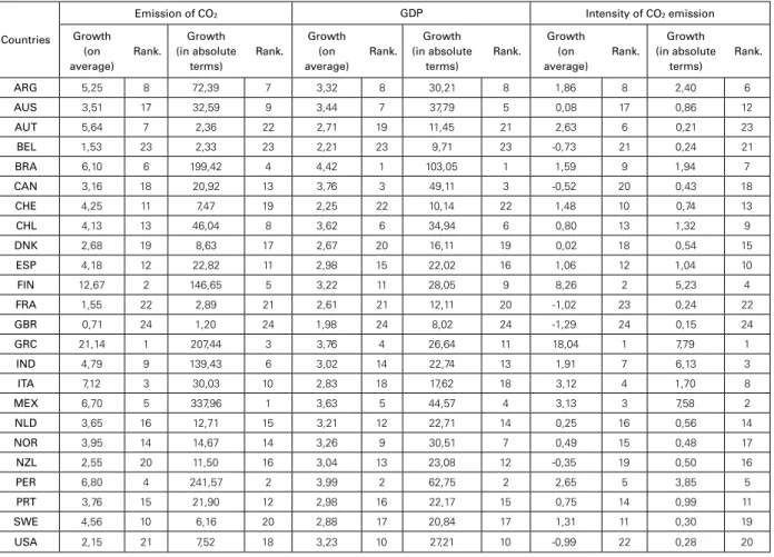
Table 1: Emission growth rate of CO2,-GDP/CO2-GDP, 1901-2010
Countries
Emission of CO2 GDP Intensity of CO2 emission
Growth (on average) Rank. Growth (in absolute terms) Rank. Growth (on average) Rank. Growth (in absolute terms) Rank. Growth (on average) Rank. Growth (in absolute terms) Rank.
ARG 5,25 8 72,39 7 3,32 8 30,21 8 1,86 8 2,40 6
AUS 3,51 17 32,59 9 3,44 7 37,79 5 0,08 17 0,86 12
AUT 5,64 7 2,36 22 2,71 19 11,45 21 2,63 6 0,21 23
BEL 1,53 23 2,33 23 2,21 23 9,71 23 -0,73 21 0,24 21
BRA 6,10 6 199,42 4 4,42 1 103,05 1 1,59 9 1,94 7
CAN 3,16 18 20,92 13 3,76 3 49,11 3 -0,52 20 0,43 18
CHE 4,25 11 7,47 19 2,25 22 10,14 22 1,48 10 0,74 13
CHL 4,13 13 46,04 8 3,62 6 34,94 6 0,80 13 1,32 9
DNK 2,68 19 8,63 17 2,67 20 16,11 19 0,02 18 0,54 15
ESP 4,18 12 22,82 11 2,98 15 22,02 16 1,06 12 1,04 10
FIN 12,67 2 146,65 5 3,22 11 28,05 9 8,26 2 5,23 4
FRA 1,55 22 2,89 21 2,61 21 12,11 20 -1,02 23 0,24 22
GBR 0,71 24 1,20 24 1,98 24 8,02 24 -1,29 24 0,15 24
GRC 21,14 1 207,44 3 3,76 4 26,64 11 18,04 1 7,79 1
IND 4,79 9 139,43 6 3,02 14 22,74 13 1,91 7 6,13 3
ITA 7,12 3 30,03 10 2,83 18 17,62 18 3,12 4 1,70 8
MEX 6,70 5 337,96 1 3,63 5 44,57 4 3,13 3 7,58 2
NLD 3,65 16 12,71 15 3,21 12 22,71 14 0,25 16 0,56 14
NOR 3,95 14 14,67 14 3,26 9 30,51 7 0,49 15 0,48 17
NZL 2,55 20 11,50 16 3,04 13 23,08 12 -0,35 19 0,50 16
PER 6,80 4 241,57 2 3,99 2 62,75 2 2,65 5 3,85 5
PRT 3,76 15 21,90 12 2,98 16 22,17 15 0,75 14 0,99 11
SWE 4,56 10 6,16 20 2,88 17 20,84 17 1,31 11 0,30 19
USA 2,15 21 7,52 18 3,23 10 27,21 10 -0,99 22 0,28 20
Source: Elaborated by the authors themselves.
Revista de Economia P
778
Note the existence of heterogeneity between average rates of growth of CO2 emissions, while developed countries such as England, Belgium and France pres-ent an average annual emission growth rate around 1,5%, occupying the lowest positions – leading nations are Greece, Finland and Italy, the former having an average growth over 20% per annum. Regarding the evolution of emissions growth in absolute terms, Mexico turned out to have the largest increase in CO2 emissions; in 2010, for instance, 337 times its emission than 1901, while England observed the lowest one, a little higher (20%) in 2010 than 1901.
Graph 3: Temporal Evolution of Average Emission Intensity, 1901 to 2010
0.1 0.12 0.14 0.16 0.18 0.2 0.22 0.24 0.26
1901 1903 1905 1907 1909 191
1
1913 1915 1917 1919 1921 1923 1925 1927 1929 1931 1933 1935 1937 1939 1941 1943 1945 1947 1949 1951 1953 1955 1957 1959 1961 1963 1965 1967 1969 1971 1973 1975 1977 1979 1981 1983 1985 1987 1989 1991 1993 1995 1997 1999 2001 2003 2005 2007 2009
Source: Elaborated by the authors themselves.
Unlike emissions of CO2, GDP growth rate varied slightly within the countries, ranging from 4,42% in Brazil to 1,98% in England. By the way, Brazil achieved the highest absolute growth; in 2010 the economy of Brazil turned out to be 100 times greater than a century earlier. As for the growth rate of emissions, England had the lowest one in absolute terms, having its economy multiplied by 8 since 1901.
Due to the accuracy, in environmental studies, many economists make use of data from 1950 onwards. Thus, in order to differentiate the dynamic traditionally observed from that available by means of historical data, the period was split into two: the first from 1901 until 1945; the second from 1945 onwards. Both are seen in Graphs 4 and 5 which further deal with average yearly GDP growth rates vs. average yearly growth rate of CO2 emissions. It is clearly indicated that economic growth in the first half of the twentieth century is accompanied by low growth rates of emissions, whereas this relationship seems to be stressed from 1956 onwards.
779
Graph 4: Gro
wth GDP vis-à-vis a
v
erage y
early
gro
wth of CO
2 emission, 1
90 1 -1 945 ARG AUS AU T BE L BRA CAN
CHE CH
L DNK ES P FIN FRA GBR IND IT A MEX NLD NOR NZ L PER PR T SWE USA
5% 6% 7% 8% 9% 10% 11 % 12%
0% 5% 10% 15% 20% 25% 30%
CRESCIMENTTO MEDIO DO PIB
CRESCIMEN
TO
MEDIO DA
EMISSAO DE CO2
Source: Elaborated b
y the authors themselv
es.
Graph 5: Gro
wth GDP vis-à-vis a
v
erage y
early
gro
wth of CO
2 emission, 1
946-20 1 0 ARG AUS AU T BE L BR A CAN CHE CHL DNK ESP FIN FRA GBR IND IT A
MEX NLD
NOR NZ L PER PR T SWE USA
2% 3% 3% 4% 4% 5% 5% 6%
0% 2% 4% 6% 8% 10% 12%
CRESCIMENTTO MEDIO DO PIB
CRESCIMEN
TO
MEDIO DA
EMISSAO DE CO2
Source: Elaborated b
y the authors themselv
es.
For the sak
e of c
omplet
eness
, Graph 6 shows t
he rank
ing of c
ountries rega rd -ing the growth averaged rate relatively to the EI. Note that developing nations (includ ing Med iterranean count ries),
with the exclusion of Fran
ce,
o
ut
line the
highest growth averaged rate.
England,
France and the United States instead
outline rather the lowest levels.
In absolute terms,
Greece,
which leads the rank
-ing,
had its intensity multiplied by 7 between the years 1901 and 2010; England,
at the same period,
reduced its EI to 15% from what it was a century before.
A
possible other reason for roughly explaining the dynamism in EI lies at the vari
-ety of economies,
whilst including the application of less pollution-intensive tech
-nologies.
There are clear
-cut evidences to support the existence of a positive relation
-Revista de Economia P
780
ship between economic growth and increase of CO2 emissions, as well as a nega-tive move in terms of EI. All that we are saying has a very direct and vital bearing upon growth rate of CO2 emission, with (perhaps) unexpected structural breaks in the series.
Graph 6: Average yearly growth of CO2 emission, 1901-2010
-0.03 0.02 0.07 0.12 0.17
GBR FR
A
US
A
BE
L
CAN NZ
L
DNK AUS NLD NOR PR
T
CH
L
ES
P
SWE CHE BRA ARG IND AU
T
PER ITA
MEX FIN GRC
Source: Elaborated by the authors themselves.
Estimation results
To identify the trend of any time series may at first glance appear to be some-thing relatively simple. Moreover, even by simpler process of visual inspection or the accurate statistics description may be misleading hinging on the properties of the series in question. we happen to know Canjels and watson (1997), Vogelsang (1998) efforts in testing the existence of deterministic trend in macroeconomics series.
In addition, there is something to be learned from the classical framework of environmental economics, because, after all, Fomby and Vogelsang (2002), Vogel-sang and Franses (2005), Coggin (2010) works are all glimpsing into the underly-ing hypothetical linear move of average growth temperature.
The increase in the global average temperature, about 0.5º every 100 years, is a remarkable result purposed in Vogelsang-Fomby 2002 paper. Further, it is worth noting that a positive trend in monthly temperatures during the winter is explicitly stated in Vogelsang-Franses (2005). Coggin (2010), in turn, applies a series of econometric tests to global and hemispheric surface temperature data. The author concludes that the tests are consistent regarding the warming pattern in recent years (post-1975).
Following Irffi 2011 paper, this study estimates the existence of any trend in EI:
y
t=∝ +
β
t
+
u
t (1)where yt denotes the EI logarithm, then β catches the deterministic trend, ut is
the error term, subscript t meaning time, measured in years, t = 1, ... ,T.
In such structure, to verify the presence of EI trend is equivalent to test H_0: β
781 = 0 vis-à-vis H_1: β ≠ 0. If the null hypothesis is rejected, the sign of β indicates the trend direction. For β > 0, it is inferred that GDP growth is accompanied by an increase in CO2 emissions. If β < 0, the country instead reversed the trend emission. Finally, if the null hypothesis is not rejected, the emission is statistically constant. To estimate its growth rate (namely, β ), the Feasible Quasi-generalized Least Squares
method developed by Perron and yabu (2009a) is taken into account. Here the trend slope is mean to be unknown pattern, that is, it can be stationary or contain a unit root. This method allows us to make inference about the slope parameter by assum-ing the standard normal distribution.
Time series lack structural changes and this may invalidate the results of sta-tistical test if they are not properly modeled. Perron-yabu test (2009b) nonetheless captures the existence of structural changes within EI trend. This test is an inspira-tion of Perron-yabu (2009a).
Given structural changes, the break date is obtained by inserting a dummy into the regression for minimizing the sum of squared error, as follows:
y t DT e T t TB t TB
t =∝ +β1 +β2 + t, where: =
(
>)
(
−)
(1)Being D a variable that captures structural change, TB assures shift date. The test statistic is part of Feasible Quasi-generalized Least Squares carrying a super-efficient estimator with known break dates from the wald test (asymptotically distributed as a qui-square random variable). On the other hand, as for unknown break dates, there are constraints, since the test statistic still hinges on the twofold aspect of the series, namely, I (0) and I (1). Moreover, the date of structural change is estimated endogenously. Further, asymptotic critical values are very close at all levels of significance, thus allowing a very asymptotical procedure as for I (0) and I (1). In addition, the simulations performed by Perron-yabu (2009a, 2009b) show greater robustness than the existing tests.
ANALyTICAL DISCUSSION OF RESULTS
we begin our analysis in this section by presenting results. All emission inten-sities measured in the manner of Perron-yabu (2009a) are initially reported, be-cause its advantages at present are huge, especially as for CO2 emission trend, by dismissing hopelessly inadequate talk of its stationarity. Subsequently, the results are estimated in the light of Perron-yabu (2009b) machinery, whose aim lies in detecting the presence of structural changes (these are very common to longer time series).
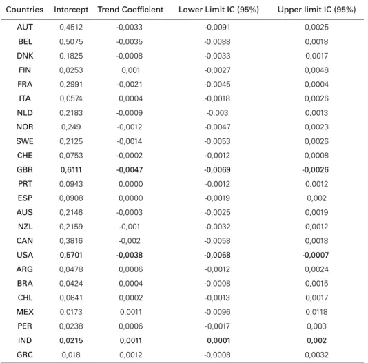
Statistically speaking, the first result, as seen in Table 2, suggests that for the most countries EI is constant, as they do not reject the null hypothesis, being the trend coefficient equal to zero forming 95% confidence interval. The exceptions are the United States, UK and India – outlining a negative trend in the two former
782
cases, whereas in the latter a positive one. In view of this picture, it can be inferred that the two developed countries, in contrast with India, are remarkably more ef-ficient in terms of emission per product generated, as India.
Table 2: Trend Estimation of CO2/GDP, Perron-Yabu (2009a)
Countries Intercept Trend Coefficient Lower Limit IC (95%) Upper limit IC (95%)
AUT 0,4512 -0,0033 -0,0091 0,0025
BEL 0,5075 -0,0035 -0,0088 0,0018
DNK 0,1825 -0,0008 -0,0033 0,0017
FIN 0,0253 0,001 -0,0027 0,0048
FRA 0,2991 -0,0021 -0,0045 0,0004
ITA 0,0574 0,0004 -0,0018 0,0026
NLD 0,2183 -0,0009 -0,003 0,0013
NOR 0,249 -0,0012 -0,0047 0,0023
SWE 0,2125 -0,0014 -0,0053 0,0026
CHE 0,0753 -0,0002 -0,0012 0,0008
GBR 0,6111 -0,0047 -0,0069 -0,0026
PRT 0,0943 0,0000 -0,0012 0,0012
ESP 0,0908 0,0000 -0,0019 0,002
AUS 0,2146 -0,0003 -0,0025 0,0019
NZL 0,2159 -0,001 -0,0032 0,0012
CAN 0,3816 -0,002 -0,0058 0,0018
USA 0,5701 -0,0038 -0,0068 -0,0007
ARG 0,0478 0,0006 -0,0012 0,0024
BRA 0,0424 0,0004 -0,0008 0,0015
CHL 0,0641 0,0002 -0,0013 0,0017
MEX 0,0173 0,0011 -0,0096 0,0118
PER 0,0238 0,0006 -0,0017 0,003
IND 0,0215 0,0011 0,0001 0,002
GRC 0,018 0,0012 -0,0008 0,0032
Source: Elaborated by the authors themselves.
yet it should be noted that, although the series earlier analyzed (see Graph 3) highlight a kind of downward moving trend as for emission intensity, Table 3 rather reports that in most countries there is no trend which be in turn statisti-cally significant. Graphs 7 and 8 report the deterministic trend coefficients as well as the 95% estimated confidence interval. Once again, the United States and UK have negative growth rates, being their absolute values remarkably observed. As extreme case, India is the unique country that showed a positive trend regarding the base period, whose economic growth is clearly intensive in EI.
783
Graph 7: Gro
wth rate of EI
-0.07 -0.05 -0.03 -0.01 0.01 0.03 0.05 0.07
GBR AUT FRA BEL USA SWE CAN NOR NZL DNK NLD CHE AUS PRT ESP CHL ITA BRA ARG PER FIN IND MEX GRC
Source: Elaborated b
y the authors themselv
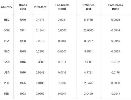
es. So far , we have only reported results with no break, thus we will also include th e po ssib ilit
y of str
uctu ral chan ge. Reg ardi ng tr end es tima tion s, T
able 3 co
nte
m
-plates pre(post)-structural change as well as its date and the statistical test.
Further
,
among the 24 countries,
eight of them presented structural change over the base
period.
Graph 8: 95% confidence inter
v
al
of CO
2 intensit
y trend
-0.01 -0.005
0
0.005 0.01
GBR USA BEL AUT FRA CAN SWE NOR NZL NLD DNK AUS CHE PRT ESP CHL ITA BRA ARG PER FIN MEX IND GRC
Source: Elaborated b
y the authors themselv
es.
The break dates indicate periods of
changement,
which in turn acknowledge
occurrences in the dynamic relationship between economic growth and emission
of
C
O
2. Fo
r ex am ple , chr on olo gi cal ly , t he U nit ed S tat es i
s a ve
ry yo ung n at ion com pa re d t o m os t o th er na tio ns o f t he wo rl d. Ho we ve r, No rt h A me ric an s h av e
developed a strong sense of pride in many areas.
For example,
in the 1910s,
North
Americans got into rival disputes with several Central
American countries,
because
they wanted to get rid of Panama’
s Canal under German influence.
As it were,
US economy is highly protectionist,
so as North
Americans were
obligated to provide primary material to their allies.
Mauro (1973) suggests that
Revista de Economia P
784
the production of coal was the most affected activity by such official control. At that time, coal turned out to be a domestic product, which should be rationed since then. Details about this can be seen in Graph 9 below.
Table 3: Structural shift and estimations-tests trend of CO2 /GDP, Perron-Yabu (2009b)
Country Break
date Intercept
Pre-break trend
Statistical test
Post-break trend
BEL 1930 0,4875 0,0021 5,5468 -0,0079
DNK 1971 0,1844 0,0007 25,0660 -0,0044
FRA 1930 0,2918 0,0011 8,8267 -0,0045
NLD 1975 0,2356 -0,0001 5,9551 -0,0035
CAN 1916 0,3685 0,0111 7,3599 -0,0152
USA 1916 0,5548 0,0116 4,4781 -0,0178
PER 1925 0,0185 0,006 2,8474 -0,0068
IND 1993 0,0209 0,0017 2,0490 -0,0041
Source: The critical value for structural break test at the 5% level counts 1.67.
Occasionally, North Americans began to engage in environmental policies, es-pecially the ones envisaged to protect forests and archaeological sites. Then they decided to build, in 1916, the National Park Service (Robertson, 1967). And, of course, this reflects a social worry about the conservation of natural resources, as Dinda (2004) points out, responsible for regulating certain sectors and so leading to a reduction of CO2 emissions.
In the light of structural change machinery, the data suggest a kind of reverse trend motived simultaneously by the fall in production of North American coal (in part due to the First world war), and the increase of environmental regulation – which restrained the intensive use of wood as source of energy.
785
Graph 9: Proportion of Emissions from Solid Fuels, USA, 1914 to 1918
89.1%
88.9%
88.7%
88.8%
88.9%
88.5% 88.6% 88.7% 88.8% 88.9% 89.0% 89.1%
1914 1915 1916 1917 1918
Source: Elaborated by the authors themselves.
The interwar period, also known as the Great Depression, shakes profoundly the world markets, in particular by reducing both production and international trade. In the European context, the countries – which were still recovering from the disasters of the First world war – faced credit shortages immediately after the fall of New york Stock Exchange, plunged into crisis once again (Mauro, 1973).
In France, for example, that picture rendered indeed grave in virtue of party clashes and popular unrest. The fifteen years that followed the crisis of 1929, until the end of the Second world war, were stagnant for the French economy. It is no coincidence at all that in the same period the EI has fallen. However, the post-war period began a race for European reconstruction with a strong GDP recovery, but it was not accompanied by the increase in emissions. This is most readily seen in Graph 10.
Furthermore, oil shocks in the 1970s meant increases in commodity prices within OPEC members. These events highlighted global fuel trade weakness – a highly concentrated sector – and so encourage the search for alternative sources of energy (Farias and Sellitto, 2011). Since then, there was a great deal in news ways of human production, consequently, less pollution-intensive.
Unlike other dates, which mark worldwide events, the structural change underlined India data occurs in a peaceful (prosperous) period. This local phe-nomenon can be explained according to Barbosa (2008) by the profound eco-nomic reforms made in the early 1990s, when liberalization and trade liberaliza-tion policies were adopted. These reforms assured a significant growth to the Indian economy with the installation of a productive sector focused on manufac-tured goods exportation. In Beckerman’s view (1992), India seems to be following the more natural way to reduce EI, and as consequence, will become a more de-veloped country.
786
Graph 10: Change in GDP and CO2
Emissions for France, 1901 to 2010
0 200 400 600 800 1000 1200 1400
1901 1903 1905 1907 1909 1911 1913 1915 1917 1919 1921 1923 1925 1927 1929 1931 1933 1935 1937 1939 1941 1943 1945 1947 1949 1951 1953 1955 1957 1959 1961 1963 1965 1967 1969 1971 1973 1975 1977 1979 1981 1983 1985 1987 1989 1991 1993 1995 1997 1999 2001 2003 2005 2007 2009
Source: Elaborated by the authors themselves.
CONCLUDING REMARKS
The foregoing sections have followed up the hazards of pollution in the domain of the society. we should supplement this now by calling Acemoglu et al. (2012) disturbing words concerning the most pressing challenges of environmental eco-nomics, though our argument lies outside the range of this controversy. we were engaged in estimating the emission intensity of CO2 having a set of 24 countries.
Admittedly, as the results showed, the most development economies, namely, the United States and United Kingdom outline altogether a consistent gain in effi-ciency. what has been said of them, however, does not apply equally to India, whose production of CO2 emission is quite high. This corresponds with its process of commercial ouverture since 1993.
Such reduction teaches us that richer countries are in line with Environmental Kuznets Curve thought by Grossman and Krueger (1991, 1995). This finding es-tablishes that post-industrial economies tend to embrace lower levels of pollution, regarding the wealth generation is altogether related to service sector. Such sector admittedly minimizes the discharge of pollutants and produces cleaner technology. The clear conclusion emerging from these data sets is that the EI path change had different origins within the countries under analysis. In addition, these chang-es appear to be tied to the changchang-es in international scenario, such as wars or supply shocks, which require a reasonable way of using natural resources, in particular, energy resources. Bearing in mind the developed countries, changes in interna-tional scenario encourage the development of more efficient means of production, thus causing a reduction in emission intensity.
Finally, as suggestion for reducing global emissions of CO2, one should take into account particular economics traits between developing and developed countries, not only by imposing them goals on increasing emissions, such proposed by Kyoto Protocol, but creating means of disseminating less emission-intensive technologies.
787 REFERENCES
ACEMOGLU, D.; AGHION, P.; BURSZTyN, L.; HEMOUS, D. (2012) “The environment and directed technical change.” American Economic Review, v. 102, p. 131-66.
ANG, B. w. (1999) “Is the energy intensity a less useful indicator than the carbon factor in the study of climate change?” Energy Policy, v. 27, p. 943-946.
ARROw, K. et al. (1995) “Economic growth, carrying capacity and the environment”. Ecological
Eco-nomics, v. 15, n. 2, p. 91–95.
BARBOSA, M. J. (2008) “Crescimento econômico da Índia antes e depois das reformas de 1985/1993”. Dissertação. Mestrado em Economia do Desenvolvimento. PUC Rio Grande do Sul, Porto Alegre. BECKERMAN, w. (1992) “Economic growth and the environment: whose growth? whose
environ-ment?” World Development, v. 20, n. 4, p. 481-496.
BODEN, T. A.; MARLAND, G.; ANDRES, R. J. (2010) “Global, regional, and national fossil-fuel CO2 emissions”. Carbon Dioxide Information Analysis Center, Oak Ridge National Laboratory, U.S. Department of Energy, Oak Ridge, Tenn., U.S.A.
BOLT, J.; ZANDEN, J. L. (2013) “The first update of Maddison Project: Re-estimating growth before 1820”. Available at <http://www.ggdc.net/maddison/maddison-project/publications/wp4.pdf>. May 2014.
CANJELS, E.; wATSON, M. w. (1997) “Estimating deterministic trends in the presence of serially correlated errors”. The Review of Economics and Statistics, v. 79, n. 2, p. 184-200.
COGGIN, T. D. (2010) “Using econometric methods to test for trends in the HadCRUT3 global and hemispheric data”. International Journal of Climatology.
COLE, M. A. (2004) “Trade, the pollution haven hypothesis and the environmental Kuznets curve: examining the linkages”. Ecological Economics, v. 48, p. 71-81.
D’ARGE, R. C.; KOGIKU, K. C. (1973) “Economic growth and the environment”. The Review of
Economic Studies, v. 40, n. 1, p. 61-77.
DINDA, S. (2004) “Environmental Kuznets Curve Hypothesis: A Survey”. Ecological Economics, v. 49, p. 431-455.
FARIAS, L. M.; SELLITTO, M. A. (2011) “Uso da energia ao longo da história: evolução e perspectivas futuras”. Revista Liberato, v. 2, n. 17, p. 01-16.
FOMBy, T.; VOGELSANG, T. J. (2002) “The application of size-robust trend statistics to global war-ming temperature series”. Journal of Climate, v. 15, p. 117–123.
GOLDEMBERG, J. (1996) “Note on the energy intensity of developing countries”. Energy Policy, v. 24, n. 8, p. 759-761.
GROSSMAN, G.; KRUEGER, A. (1991) “Environmental impacts of a North American free trade agre-ement”. NBER, paper 3914, Cambridge, MA.
GROSSMAN, G.; KRUEGER, A. (1995) “Economic growth and the environment”. Quarterly Journal
of Economics, v. 110, n. 2, p. 353-377.
IPCC (Intergovernmental Panel on Climate Change). (2001) Climate Change 2001: The Scientific Basis. Cambridge, UK: Cambridge University Press.
IPCC (Intergovernmental Panel on Climate Change). (2003) Draft Report on the 21st Session of the
IPCC. Vienna: mimeo. Available at <www.ipcc.ch> [May 2014].
IPCC (Intergovernmental Panel on Climate Change). (2000). Special Report on Emissions Scenarios. Cambridge, UK: Cambridge University Press.
IRFFI, G. D. (2011) “Ensaios sobre a relação entre Emissão de CO2 e a Renda Global”. Tese (Douto-rado) – CAEN, Pós Graduação em Economia. Universidade Federal do Ceará, Fortaleza. MAURO, F. (1973) História da Economia Mundial 1790-1970. Rio de Janeiro: Zahar.
MIELNIK, O.; GOLDEMBERG, J. (1999) “The evolution of the carbonization index in developing countries”. Energy Policy, v. 27, p. 307- 308.
NIELSSON, L. (1993) “Energy intensity in 31 industrial and developing countries 1950-88”. Energy, v. 18, p. 309-322.
788
PERRON, P.; yABU T. (2009a) “Estimating deterministic trends with an integrated or stationary noise component”. Journal of Econometrics, v. 151, p. 56–69.
PERRON, P.; yABU T. (2009b) “Testing for shifts in trend with an integrated or stationary noise com-ponent” . Journal of Business and Economic Statistics, v. 27, p. 369–396.
ROBERTSON, R. M. (1967) História da Economia Americana. v. 2. Rio de Janeiro: Record.
ROCA, J.; ALCáNTARA, V. (2001) “Energy intesity, CO2 emissions and the environmental Kuznets
curve. The Spanish case”. Energy Policy, v. 29, p. 553-556.
STERN, D. I. (1998) “Progress on the environmental Kuznets curve?” Environmental and Development
Economics, v. 3, n. 2, p. 173-196.
SURI, V.; CHAPMAN, D. (1998) “Economic growth, trade and energy: implications for the environ-mental Kuznets curve”. Ecological Economics, v. 25, p. 195-208.
VOGELSANG, T. J. (1998) “Trend function hypothesis testing in the presence of serial correlation”.
Econometrica, v. 66, p. 123–148.
VOGELSANG, T. J.; FRANSES, P. H. (2005) “Testing for common deterministic trend slopes”. Journal
of Econometrics, v. 126, n. 1, p. 1-24.