Elements of Applied
Bifurcation Theory,
Second Edition
Yuri A. Kuznetsov
Preface to the Second Edition
The favorable reaction to the first edition of this book confirmed that the publication of such an application-oriented text on bifurcation theory of dynamical systems was well timed. The selected topics indeed cover ma-jor practical issues of applying the bifurcation theory to finite-dimensional problems. This new edition preserves the structure of the first edition while updating the context to incorporate recent theoretical developments,in particular,new and improved numerical methods for bifurcation analysis. The treatment of some topics has been clarified.
Two- and three-dimensional cases are treated in the main text,while the analysis of bifurcations in four-dimensional systems with a homoclinic orbit to a focus-focus is outlined in the new appendix. In Chapter 7,an explicit example of the “blue sky” bifurcation is discussed. Chapter 10,devoted to the numerical analysis of bifurcations,has been changed most substantially. We have introduced bordering methods to continue fold and Hopf bifur-cations in two parameters. In this approach,the defining function for the bifurcation used in the minimal augmented system is computed by solving a bordered linear system. It allows for explicit computation of the gradi-ent of this function,contrary to the approach when determinants are used as the defining functions. The main text now includes BVP methods to continue codim 1 homoclinic bifurcations in two parameters,as well as all codim 1 limit cycle bifurcations. A new appendix to this chapter provides test functions to detect all codim 2 homoclinic bifurcations involving a sin-gle homoclinic orbit to an equilibrium. The software review in Appendix 3 to this chapter is updated to present recently developed programs,in-cluding AUTO97 with HomCont,DsTool,and CONTENT providing the information on their availability by ftp.
A number of misprints and minor errors have been corrected while prepar-ing this edition. I would like to thank many colleagues who have sent comments and suggestions,including E. Doedel (Concordia University, Montreal),B. Krauskopf (VU,Amsterdam),S. van Gils (TU Twente,En-schede),B. Sandstede (WIAS,Berlin),W.-J. Beyn (Bielefeld University), F.S. Berezovskaya (Center for Ecological Problems and Forest Productivity, Moscow),E. Nikolaev and E.E. Shnoll (IMPB,Pushchino,Moscow Region), W. Langford (University of Guelph),O. Diekmann (Utrecht University), and A. Champneys (University of Bristol).
I am thankful to my wife,Lioudmila,and to my daughters,Elena and Ouliana,for their understanding,support,and patience,while I was work-ing on this book and developwork-ing the bifurcation software CONTENT.
Finally,I would like to acknowledge the Research Institute for Applica-tions of Computer Algebra (RIACA,Eindhoven) for the financial support of my work at CWI (Amsterdam) in 1995–1997.
Preface to the First Edition
During the last few years,several good textbooks on nonlinear dynam-ics have appeared for graduate students in applied mathematdynam-ics. It seems, however,that the majority of such books are still too theoretically ori-ented and leave many practical issues unclear for people intending to apply the theory to particular research problems. This book is designed for ad-vanced undergraduate or graduate students in mathematics who will par-ticipate in applied research. It is also addressed to professional researchers in physics,biology,engineering,and economics who use dynamical systems as modeling tools in their studies. Therefore,only a moderate mathematical background in geometry,linear algebra,analysis,and differential equations is required. A brief summary of general mathematical terms and results, which are assumed to be known in the main text,appears at the end of the book. Whenever possible,only elementary mathematical tools are used. For example,we do not try to present normal form theory in full general-ity,instead developing only the portion of the technique sufficient for our purposes.
The book aims to provide the student (or researcher) with both a solid basis in dynamical systems theory and the necessary understanding of the approaches,methods,results,and terminology used in the modern applied mathematics literature. A key theme is that oftopological equivalence and
nonlin-ear dynamical systems or systems theory. Certain classical results,such as Andronov-Hopf and homoclinic bifurcation in two-dimensional systems, are presented in great detail,including self-contained proofs. For more com-plex topics of the theory,such as homoclinic bifurcations in more than two dimensions and two-parameter local bifurcations,we try to make clear the relevant geometrical ideas behind the proofs but only sketch them or,some-times,discuss and illustrate the results but give only references of where to find the proofs. This approach,we hope,makes the book readable for a wide audience and keeps it relatively short and able to be browsed. We also present several recent theoretical results concerning,in particular,bifurca-tions of homoclinic orbits to nonhyperbolic equilibria and one-parameter bifurcations of limit cycles in systems with reflectional symmetry. These results are hardly covered in standard graduate-level textbooks but seem to be important in applications.
In this book we try to provide the reader with explicit procedures for application of general mathematical theorems to particular research prob-lems. Special attention is given to numerical implementation of the devel-oped techniques. Several examples,mainly from mathematical biology,are used as illustrations.
The present text originated in a graduate course on nonlinear systems taught by the author at the Politecnico di Milano in the Spring of 1991. A similar postgraduate course was given at the Centrum voor Wiskunde en Informatica (CWI,Amsterdam) in February,1993. Many of the examples and approaches used in the book were first presented at the seminars held at the Research Computing Centre1 of the Russian Academy of Sciences
(Pushchino,Moscow Region).
Let us briefly characterize the content of each chapter.
Chapter 1. Introduction to dynamical systems. In this chapter we introduce basic terminology. Adynamical system is defined geometrically as a family of evolution operators ϕt acting in some state space X and
parametrized by continuous or discrete timet. Some examples,including symbolic dynamics,are presented. Orbits,phase portraits,and invariant sets appear before any differential equations,which are treated as one of the ways to define a dynamical system. The Smale horseshoe is used to illus-trate the existence of very complex invariant sets having fractal structure. Stability criteria for the simplest invariant sets (equilibria and periodic or-bits) are formulated. An example of infinite-dimensional continuous-time dynamical systems is discussed,namely,reaction-diffusion systems.
Chapter 2. Topological equivalence, bifurcations, and structural stability of dynamical systems. Two dynamical systems are called topo-logically equivalentif their phase portraits are homeomorphic. This notion is
1Renamed in 1992 as the Institute of Mathematical Problems of Biology
Preface to the First Edition xi
then used to define structurally stable systems and bifurcations. The topo-logical classification of generic (hyperbolic) equilibria and fixed points of dynamical systems defined by autonomous ordinary differential equations (ODEs) and iterated maps is given,and the geometry of the phase portrait near such points is studied. Abifurcation diagramof a parameter-dependent system is introduced as a partitioning of its parameter space induced by the topological equivalence of corresponding phase portraits. We introduce the notion ofcodimension (codim for short) in a rather naive way as the number of conditions defining the bifurcation. Topological normal forms
(universal unfoldings of nondegenerate parameter-dependent systems) for bifurcations are defined,and an example of such a normal form is demon-strated for the Hopf bifurcation.
Chapter 3. One-parameter bifurcations of equilibria in continu-ous-time dynamical systems. Two generic codim 1 bifurcations – tan-gent (fold)and Andronov-Hopf – are studied in detail following the same general approach: (1) formulation of the corresponding topological normal form and analysis of its bifurcations; (2) reduction of a generic parameter-dependent system to the normal form up to terms of a certain order; and (3) demonstration that higher-order terms do not affect the local bifur-cation diagram. Step 2 (finite normalization) is performed by means of polynomial changes of variables with unknown coefficients that are then fixed at particular values to simplify the equations. Relevant normal form and nondegeneracy (genericity) conditions for a bifurcation appear natu-rally at this step. An example of the Hopf bifurcation in a predator-prey system is analyzed.
Chapter 4. One-parameter bifurcations of fixed points in discre-te-time dynamical systems. The approach formulated in Chapter 3 is applied to studytangent (fold),flip(period-doubling),andHopf( Neimark-Sacker) bifurcations of discrete-time dynamical systems. For the Neimark-Sacker bifurcation,as is known,a normal form so obtained captures only the appearance of a closed invariant curve but does not describe the orbit structure on this curve. Feigenbaum’s universality in the cascade of period doublings is explained geometrically using saddle properties of the period-doubling map in an appropriate function space.
Chapter 5. Bifurcations of equilibria and periodic orbits in n
method,we derive a compact formula to determine the direction of a Hopf bifurcation in multidimensional systems. Finally,we consider a reaction-diffusion system on an interval to illustrate the necessary modifications of the technique to handle the Hopf bifurcation in some infinite-dimensional systems.
Chapter 6. Bifurcations of orbits homoclinic and heteroclinic to hyperbolic equilibria. This chapter is devoted to the generation of periodic orbits via homoclinic bifurcations. A theorem due to Andronov and Leontovich describing homoclinic bifurcation in planar continuous-time systems is formulated. A simple proof is given which uses a constructive
C1-linearization of a system near its saddle point. All codim 1 bifurcations
of homoclinic orbits to saddle and saddle-focus equilibrium points in three-dimensional ODEs are then studied. The relevant theorems by Shil’nikov are formulated together with the main geometrical constructions involved in their proofs. The role of the orientability of invariant manifolds is em-phasized. Generalizations to more dimensions are also discussed. An appli-cation of Shil’nikov’s results to nerve impulse modeling is given.
Chapter 7. Other one-parameter bifurcations in continuous-time dynamical systems. This chapter treats some bifurcations of ho-moclinic orbits to nonhyperbolic equilibrium points,including the case of several homoclinic orbits to a saddle-saddle point,which provides one of the simplest mechanisms for the generation of an infinite number of peri-odic orbits. Bifurcations leading to a change in the rotation number on an invariant torus and some other global bifurcations are also reviewed. All codim 1 bifurcations of equilibria and limit cycles inZ2-symmetric systems
are described together with their normal forms.
Chapter 8. Two-parameter bifurcations of equilibria in conti-nuous-time dynamical systems. One-dimensional manifolds in the di-rect product of phase and parameter spaces corresponding to the tangent and Hopf bifurcations are defined and used to specify all possible codim 2 bifurcations of equilibria in generic continuous-time systems. Topological normal forms are presented and discussed in detail for the cusp,Bogdanov-Takens,and generalized Andronov-Hopf (Bautin) bifurcations. An example of a two-parameter analysis of Bazykin’s predator-prey model is considered in detail. Approximating symmetric normal forms for zero-Hopf and Hopf-Hopf bifurcations are derived and studied,and their relationship with the original problems is discussed. Explicit formulas for the critical normal form coefficients are given for the majority of the codim 2 cases.
Preface to the First Edition xiii
in terms of continuous-time planar dynamical systems for all strong reso-nances (1:1,1:2,1:3,and 1:4). The Taylor coefficients of these continuous-time systems are explicitly given in terms of those of the maps in question. A periodically forced predator-prey model is used to illustrate resonant phenomena.
Chapter 10. Numerical analysis of bifurcations. This final chapter deals with numerical analysis of bifurcations,which in most cases is the only tool to attack real problems. Numerical procedures are presented for the location and stability analysis of equilibria and the local approximation of their invariant manifolds as well as methods for the location of limit cycles (including orthogonal collocation). Several methods are discussed for equilibrium continuation and detection of codim 1 bifurcations based on predictor-corrector schemes. Numerical methods for continuation and analysis of homoclinic bifurcations are also formulated.
Each chapter contains exercises,and we have provided hints for the most difficult of them. The references and comments to the literature are sum-marized at the end of each chapter as separate bibliographical notes. The aim of these notes is mainly to provide a reader with information on fur-ther reading. The end of a theorem’s proof (or its absence) is marked by the symbol ✷,while that of a remark (example) is denoted by ♦ (✸), respectively.
As is clear from this Preface,there are many important issues this book does not touch. In fact,we study only the first bifurcations on a route to chaos and try to avoid the detailed treatment of chaotic dynamics,which requires more sophisticated mathematical tools. We do not consider im-portant classes of dynamical systems such as Hamiltonian systems (e.g., KAM-theory and Melnikov methods are left outside the scope of this book). Only introductory information is provided on bifurcations in systems with symmetries. The list of omissions can easily be extended. Nevertheless,we hope the reader will find the book useful,especially as an interface between undergraduate and postgraduate studies.
of the University of Bristol,who reviewed the whole text and not only cor-rected the language but also proposed many improvements in the selection and presentation of the material. Certain topics have been discussed with J. Sanders (VU/RIACA/CWI,Amsterdam),B. Werner (University of Ham-burg),E. Nikolaev (IMPB,Pushchino),E. Doedel (Concordia University, Montreal),B. Sandstede (IAAS,Berlin),M. Kirkilonis (CWI,Amsterdam), J. de Vries (CWI,Amsterdam),and others,whom I would like to thank. Of course,the responsibility for all remaining mistakes is mine. I would also like to thank A. Heck (CAN,Amsterdam) and V.V. Levitin (IMPB, Pushchino/CWI,Amsterdam) for computer assistance. Finally,I thank the Nederlandse Organisatie voor Wetenschappelijk Onderzoek (NWO) for pro-viding financial support during my stay at CWI,Amsterdam.
Contents
Preface to the Second Edition vii
Preface to the First Edition ix
1 Introduction to Dynamical Systems 1
1.1 Definition of a dynamical system . . . 1
1.1.1 State space . . . 2
1.1.2 Time. . . 5
1.1.3 Evolution operator . . . 5
1.1.4 Definition of a dynamical system . . . 7
1.2 Orbits and phase portraits . . . 8
1.3 Invariant sets . . . 11
1.3.1 Definition and types . . . 11
1.3.2 Example 1.9 (Smale horseshoe) . . . 12
1.3.3 Stability of invariant sets . . . 16
1.4 Differential equations and dynamical systems . . . 18
1.5 Poincar´e maps . . . 23
1.5.1 Time-shift maps . . . 24
1.5.2 Poincar´e map and stability of cycles . . . 25
1.5.3 Poincar´e map for periodically forced systems . . . . 30
1.6 Exercises . . . 31
1.7 Appendix 1: Infinite-dimensional dynamical systems defined by reaction-diffusion equations . . . 33
2 Topological Equivalence, Bifurcations,
and Structural Stability of Dynamical Systems 39
2.1 Equivalence of dynamical systems. . . 39
2.2 Topological classification of generic equilibria and fixed points 46 2.2.1 Hyperbolic equilibria in continuous-time systems . . 46
2.2.2 Hyperbolic fixed points in discrete-time systems . . 49
2.2.3 Hyperbolic limit cycles. . . 54
2.3 Bifurcations and bifurcation diagrams . . . 57
2.4 Topological normal forms for bifurcations . . . 63
2.5 Structural stability . . . 68
2.6 Exercises . . . 73
2.7 Appendix: Bibliographical notes. . . 76
3 One-Parameter Bifurcations of Equilibria in Continuous-Time Dynamical Systems 79 3.1 Simplest bifurcation conditions . . . 79
3.2 The normal form of the fold bifurcation . . . 80
3.3 Generic fold bifurcation . . . 83
3.4 The normal form of the Hopf bifurcation . . . 86
3.5 Generic Hopf bifurcation. . . 91
3.6 Exercises . . . 104
3.7 Appendix 1: Proof of Lemma 3.2 . . . 108
3.8 Appendix 2: Bibliographical notes . . . 111
4One-Parameter Bifurcations of Fixed Points in Discrete-Time Dynamical Systems 113 4.1 Simplest bifurcation conditions . . . 113
4.2 The normal form of the fold bifurcation . . . 114
4.3 Generic fold bifurcation . . . 116
4.4 The normal form of the flip bifurcation. . . 119
4.5 Generic flip bifurcation. . . 121
4.6 The “normal form” of the Neimark-Sacker bifurcation . . . 125
4.7 Generic Neimark-Sacker bifurcation. . . 129
4.8 Exercises . . . 138
4.9 Appendix 1: Feigenbaum’s universality . . . 139
4.10 Appendix 2: Proof of Lemma 4.3 . . . 143
4.11 Appendix 3: Bibliographical notes . . . 149
5 Bifurcations of Equilibria and Periodic Orbits in n-Dimensional Dynamical Systems 151 5.1 Center manifold theorems . . . 151
5.1.1 Center manifolds in continuous-time systems . . . . 152
5.1.2 Center manifolds in discrete-time systems . . . 156
5.2 Center manifolds in parameter-dependent systems . . . 157
Preface to the First Edition xvii
5.4 Computation of center manifolds . . . 165
5.4.1 Quadratic approximation to center manifolds in eigenbasis . . . 165
5.4.2 Projection method for center manifold computation 171 5.5 Exercises . . . 186
5.6 Appendix 1: Hopf bifurcation in reaction-diffusion systems on the interval with Dirichlet boundary conditions . . . 189
5.7 Appendix 2: Bibliographical notes . . . 193
6 Bifurcations of Orbits Homoclinic and Heteroclinic to Hyperbolic Equilibria 195 6.1 Homoclinic and heteroclinic orbits . . . 195
6.2 Andronov-Leontovich theorem. . . 200
6.3 Homoclinic bifurcations in three-dimensional systems: Shil’nikov theorems. . . 213
6.4 Homoclinic bifurcations in n-dimensional systems . . . 228
6.4.1 Regular homoclinic orbits: Melnikov integral . . . . 229
6.4.2 Homoclinic center manifolds. . . 232
6.4.3 Generic homoclinic bifurcations in Rn . . . . 236
6.5 Exercises . . . 238
6.6 Appendix 1: Focus-focus homoclinic bifurcation in four-dimensional systems . . . 241
6.7 Appendix 2: Bibliographical notes . . . 247
7 Other One-Parameter Bifurcations in Continuous-Time Dynamical Systems 249 7.1 Codim 1 bifurcations of homoclinic orbits to nonhyperbolic equilibria . . . 250
7.1.1 Saddle-node homoclinic bifurcation on the plane . . 250
7.1.2 Saddle-node and saddle-saddle homoclinic bifurcations in R3 . . . . 253
7.2 “Exotic” bifurcations . . . 262
7.2.1 Nontransversal homoclinic orbit to a hyperbolic cycle 263 7.2.2 Homoclinic orbits to a nonhyperbolic limit cycle . . 263
7.3 Bifurcations on invariant tori . . . 267
7.3.1 Reduction to a Poincar´e map . . . 267
7.3.2 Rotation number and orbit structure . . . 269
7.3.3 Structural stability and bifurcations . . . 270
7.3.4 Phase locking near a Neimark-Sacker bifurcation: Arnold tongues . . . 272
7.4 Bifurcations in symmetric systems . . . 276
7.4.1 General properties of symmetric systems. . . 276
7.4.2 Z2-equivariant systems. . . . 278
7.4.4 Codim 1 bifurcations of cycles
in Z2-equivariant systems . . . . 283
7.5 Exercises . . . 288
7.6 Appendix 1: Bibliographical notes . . . 290
8 Two-Parameter Bifurcations of Equilibria in Continuous-Time Dynamical Systems 293 8.1 List of codim 2 bifurcations of equilibria . . . 294
8.1.1 Codim 1 bifurcation curves . . . 294
8.1.2 Codim 2 bifurcation points . . . 297
8.2 Cusp bifurcation . . . 301
8.2.1 Normal form derivation . . . 301
8.2.2 Bifurcation diagram of the normal form . . . 303
8.2.3 Effect of higher-order terms . . . 305
8.3 Bautin (generalized Hopf) bifurcation . . . 307
8.3.1 Normal form derivation . . . 307
8.3.2 Bifurcation diagram of the normal form . . . 312
8.3.3 Effect of higher-order terms . . . 313
8.4 Bogdanov-Takens (double-zero) bifurcation . . . 314
8.4.1 Normal form derivation . . . 314
8.4.2 Bifurcation diagram of the normal form . . . 321
8.4.3 Effect of higher-order terms . . . 324
8.5 Fold-Hopf (zero-pair) bifurcation . . . 330
8.5.1 Derivation of the normal form. . . 330
8.5.2 Bifurcation diagram of the truncated normal form . 337 8.5.3 Effect of higher-order terms . . . 342
8.6 Hopf-Hopf bifurcation . . . 349
8.6.1 Derivation of the normal form. . . 349
8.6.2 Bifurcation diagram of the truncated normal form . 356 8.6.3 Effect of higher-order terms . . . 366
8.7 Exercises . . . 369
8.8 Appendix 1: Limit cycles and homoclinic orbits of Bogdanov normal form . . . 382
8.9 Appendix 2: Bibliographical notes . . . 390
9 Two-Parameter Bifurcations of Fixed Points in Discrete-Time Dynamical Systems 393 9.1 List of codim 2 bifurcations of fixed points. . . 393
9.2 Cusp bifurcation . . . 397
9.3 Generalized flip bifurcation . . . 400
9.4 Chenciner (generalized Neimark-Sacker) bifurcation. . . 404
9.5 Strong resonances. . . 408
9.5.1 Approximation by a flow . . . 408
9.5.2 1:1 resonance . . . 410
Preface to the First Edition xix
9.5.4 1:3 resonance . . . 428
9.5.5 1:4 resonance . . . 435
9.6 Codim 2 bifurcations of limit cycles. . . 446
9.7 Exercises . . . 457
9.8 Appendix 1: Bibliographical notes . . . 460
10 Numerical Analysis of Bifurcations 463 10.1 Numerical analysis at fixed parameter values . . . 464
10.1.1 Equilibrium location . . . 464
10.1.2 Modified Newton’s methods . . . 466
10.1.3 Equilibrium analysis . . . 469
10.1.4 Location of limit cycles . . . 472
10.2 One-parameter bifurcation analysis . . . 478
10.2.1 Continuation of equilibria and cycles . . . 479
10.2.2 Detection and location of codim 1 bifurcations . . . 484
10.2.3 Analysis of codim 1 bifurcations . . . 488
10.2.4 Branching points . . . 495
10.3 Two-parameter bifurcation analysis. . . 501
10.3.1 Continuation of codim 1 bifurcations of equilibria and fixed points . . . 501
10.3.2 Continuation of codim 1 limit cycle bifurcations . . 507
10.3.3 Continuation of codim 1 homoclinic orbits . . . 510
10.3.4 Detection and location of codim 2 bifurcations . . . 514
10.4 Continuation strategy . . . 515
10.5 Exercises . . . 517
10.6 Appendix 1: Convergence theorems for Newton methods . . 525
10.7 Appendix 2: Detection of codim 2 homoclinic bifurcations . 526 10.7.1 Singularities detectable via eigenvalues . . . 527
10.7.2 Orbit and inclination flips . . . 529
10.7.3 Singularities along saddle-node homoclinic curves . . 534
10.8 Appendix 3: Bibliographical notes . . . 535
A Basic Notions from Algebra, Analysis, and Geometry 541 A.1 Algebra . . . 541
A.1.1 Matrices . . . 541
A.1.2 Vector spaces and linear transformations. . . 543
A.1.3 Eigenvectors and eigenvalues . . . 544
A.1.4 Invariant subspaces,generalized eigenvectors, and Jordan normal form . . . 545
A.1.5 Fredholm Alternative Theorem . . . 546
A.1.6 Groups . . . 546
A.2 Analysis . . . 547
A.2.1 Implicit and Inverse Function Theorems . . . 547
A.2.2 Taylor expansion . . . 548
A.3 Geometry . . . 550
A.3.1 Sets . . . 550
A.3.2 Maps . . . 551
A.3.3 Manifolds . . . 551
References 553
1
Introduction to Dynamical Systems
This chapter introduces some basic terminology. First,we define a dynam-ical systemand give several examples,including symbolic dynamics. Then we introduce the notions of orbits, invariant sets,and their stability. As we shall see while analyzing theSmale horseshoe,invariant sets can have very complex structures. This is closely related to the fact discovered in the 1960s that rather simple dynamical systems may behave “randomly,” or “chaotically.” Finally,we discuss how differential equations can define dynamical systems in both finite- and infinite-dimensional spaces.
1.1 Definition of a dynamical system
The notion of a dynamical system is the mathematical formalization of the general scientific concept of a deterministic process. The future and past states of many physical,chemical,biological,ecological,economical,and even social systems can be predicted to a certain extent by knowing their present state and the laws governing their evolution. Provided these laws do not change in time,the behavior of such a system could be considered as completely defined by its initial state. Thus,the notion of a dynamical system includes a set of its possible states (state space) and a law of the
ϕ l
.
m ϕ
FIGURE 1.1. Classical pendulum.
1.1.1 State space
All possible states of a system are characterized by the points of some setX. This set is called thestate spaceof the system. Actually,the specification of a pointx∈Xmust be sufficient not only to describe the current “position” of the system but also to determine its evolution. Different branches of science provide us with appropriate state spaces. Often,the state space is called aphase space,following a tradition from classical mechanics.
Example 1.1 (Pendulum) The state of an ideal pendulum is
com-pletely characterized by defining its angulardisplacementϕ(mod 2π) from the vertical position and the corresponding angularvelocityϕ˙ (see Figure 1.1). Notice that the angleϕ alone is insufficient to determine the future state of the pendulum. Therefore,for this simple mechanical system,the state space isX =S1×R1,whereS1is the unit circle parametrized by the
angle,andR1is the real axis corresponding to the set of all possible
veloc-ities. The setX can be considered as a smooth two-dimensionalmanifold
(cylinder) inR3.✸
Example 1.2 (General mechanical system)In classical mechanics,
the state of an isolated system withsdegrees of freedom is characterized by a 2s-dimensional real vector:
(q1, q2, . . . , qs, p1, p2, . . . , ps)T,
where qi are the generalized coordinates,while pi are the corresponding
generalized momenta. Therefore,in this case,X =R2s. Ifkcoordinates are
cyclic,X =Sk×R2s−k. In the case of the pendulum,s=k= 1, q1 =ϕ,
and we can takep1= ˙ϕ. ✸
Example 1.3 (Quantum system)In quantum mechanics,the state of
a system withtwo observable statesis characterized by a vector
ψ=
a1 a2
1.1 Definition of a dynamical system 3
where ai, i = 1,2, are complex numbers called amplitudes,satisfying the
condition
|a1|2+|a2|2= 1.
The probability of finding the system in the ith state is equal to pi = |ai|2, i= 1,2.✸
Example 1.4(Chemical reactor)The state of a well-mixed isothermic chemical reactor is defined by specifying the volumeconcentrations of the
nreacting chemical substances
c= (c1, c2, . . . , cn)T.
Clearly,the concentrationsci must be nonnegative. Thus,
X={c:c= (c1, c2, . . . , cn)T ∈Rn, ci≥0}.
If the concentrations change from point to point,the state of the reactor is defined by the reagent distributionsci(x), i= 1,2, . . . , n. These functions
are defined in a bounded spatial domain Ω,the reactor interior,and charac-terize the local concentrations of the substances near a pointx. Therefore, the state spaceX in this case is afunction spacecomposed of vector-valued functionsc(x),satisfying certain smoothness and boundary conditions. ✸
Example 1.5 (Ecological system) Similar to the previous example,
the state of an ecological community within a certain domain Ω can be described by a vector with nonnegative components
N = (N1, N2, . . . , Nn)T ∈Rn,
or by a vector function
N(x) = (N1(x), N2(x), . . . , Nn(x))T, x∈Ω,
depending on whether the spatial distribution is essential for an adequate description of the dynamics. HereNi is the number (or density) of theith
species or other group (e.g.,predators or prey).✸
Example 1.6 (Symbolic dynamics) To complete our list of state
spaces,consider a set Ω2of all possible bi-infinitesequencesof two symbols,
say{1,2}. A pointω∈X is the sequence
ω={. . . , ω−2, ω−1, ω0, ω1, ω2, . . .},
whereωi∈ {1,2}. Note that the zero position in a sequence must be pointed
out; for example,there are two distinct periodic sequences that can be written as
one with ω0 = 1,and the other with ω0 = 2. The space Ω2 will play an
important role in the following.
Sometimes,it is useful to identify two sequences that differ only by a shift of the origin. Such sequences are calledequivalent. The classes of equivalent sequences form a set denoted byΩ2. The two periodic sequences mentioned
above represent the same point inΩ2.✸
In all the above examples,the state space has a certain natural struc-ture,allowing for comparison between different states. More specifically,a
distanceρbetween two states is defined,making these setsmetric spaces. In the examples from mechanics and in the simplest examples from chem-istry and ecology,the state space was a real vector space Rn of some
fi-nite dimension n,or a (sub-)manifold (hypersurface) in this space. The
Euclidean norm can be used to measure the distance between two states parametrized by the pointsx, y∈Rn,namely
ρ(x, y) =x−y=x−y, x−y=
n
i=1
(xi−yi)2, (1.1)
where·,·is the standard scalar product in Rn,
x, y=xTy=
n
i=1 xiyi.
If necessary,the distance between two (close) points on a manifold can be measured as the minimal length of a curve connecting these points within the manifold. Similarly,the distance between two statesψ, ϕof the quantum system from Example 1.3 can be defined using the standard scalar product inCn,
ψ, ϕ= ¯ψTϕ=
n
i=1
¯
ψiϕi,
withn= 2. Meanwhile,ψ, ψ=ϕ, ϕ= 1.
When the state space is a function space,there is a variety of possible distances,depending on thesmoothness(differentiability) of the functions allowed. For example,we can introduce a distance between two continuous vector-valued real functions u(x) and v(x) defined in a bounded closed domain Ω∈Rmby
ρ(u, v) =u−v= max
i=1,...,n xsup∈Ω|ui(x)−vi(x)|.
Finally,in Example 1.6 the distance between two sequences ω, θ ∈ Ω2
can be measured by
ρ(ω, θ) =
+∞
k=−∞
δωkθk2
1.1 Definition of a dynamical system 5
where
δωkθk =
0 if ωk=θk,
1 if ωk=θk.
According to this formula,two sequences are considered to be close if they have a long block of coinciding elements centered at position zero (check!). Using the previously defined distances,the introduced state spacesXare
complete metric spaces. Loosely speaking,this means that any sequence of states,all of whose sufficiently future elements are separated by an arbi-trarily small distance,is convergent (the space has no “holes”).
According to the dimension of the underlying state space X,the dy-namical system is called eitherfinite-orinfinite-dimensional. Usually,one distinguishes finite-dimensional systems defined inX =Rn from those
de-fined on manifolds.
1.1.2 Time
The evolution of a dynamical system means a change in the state of the system with time t ∈ T,where T is a number set. We will consider two types of dynamical systems: those with continuous (real) time T = R1,
and those with discrete (integer) time T = Z. Systems of the first type
are called continuous-time dynamical systems,while those of the second are termeddiscrete-timedynamical systems. Discrete-time systems appear naturally in ecology and economics when the state of a system at a certain moment of timetcompletely determines its state after a year,say att+ 1.
1.1.3 Evolution operator
The main component of a dynamical system is an evolution law that de-termines the statextof the system at timet,provided theinitial statex0
is known. The most general way to specify the evolution is to assume that for givent∈T a mapϕt is defined in the state spaceX,
ϕt:X→X,
which transforms an initial statex0∈X into some statext∈X at timet:
xt=ϕtx0.
The mapϕtis often called theevolution operatorof the dynamical system.
It might be known explicitly; however,in most cases,it is definedindirectly
and can be computed only approximately. In the continuous-time case,the family{ϕt}
t∈T of evolution operators is called aflow.
Note thatϕtxmay not be defined for all pairs (x, t)∈X×T. Dynamical
calledinvertible. In such systems the initial statex0completely defines not only thefuturestates of the system,but itspastbehavior as well. However, it is useful to consider also dynamical systems whose future behavior fort >
0 is completely determined by their initial statex0att= 0,but the history for t < 0 can not be unambigously reconstructed. Such (noninvertible) dynamical systems are described by evolution operators defined only for
t≥0 (i.e.,fort∈R1+ orZ+). In the continuous-time case,they are called
semiflows.
It is also possible thatϕtx0 is defined onlylocally in time,for example,
for 0 ≤ t < t0,where t0 depends on x0 ∈ X. An important example of such a behavior is a “blow-up,” when a continuous-time system inX =Rn
approaches infinity within a finite time,i.e.,
ϕtx0 →+∞,
fort→t0.
The evolution operators have two natural properties that reflect the de-terministic character of the behavior of dynamical systems. First of all,
(DS.0) ϕ0= id,
where id is the identity map onX, idx=xfor all x∈X. The property (DS.0) implies that the system does not change its state “spontaneously.” The second property of the evolution operators reads
(DS.1) ϕt+s=ϕt◦ϕs.
It means that
ϕt+sx=ϕt(ϕsx)
for all x ∈ X and t, s ∈ T, suchthat bothsides of the last equation are defined.1 Essentially,the property (DS.1) states that the result of the
evo-lution of the system in the course oft+sunits of time,starting at a point
x∈X,is the same as if the system were first allowed to change from the state xover only s units of time and then evolved over the next t units of time from the resulting stateϕsx(see Figure 1.2). This property means
that the law governing the behavior of the system does not change in time: The system is “autonomous.”
For invertible systems,the evolution operator ϕt satisfies the property
(DS.1) for t and s both negative and nonnegative. In such systems,the operatorϕ−tis the inverse toϕt, (ϕt)−1=ϕ−t,since
ϕ−t◦ϕt= id.
1Whenever possible, we will avoid explicit statements on the domain of
1.1 Definition of a dynamical system 7
ϕ
x
t
x
x
0
s
t+s
X
ϕ
s
FIGURE 1.2. Evolution operator.
A discrete-time dynamical system with integer t is fully specified by defining only one mapf =ϕ1,called“time-one map.”Indeed,using (DS.1),
we obtain
ϕ2=ϕ1◦ϕ1=f◦f =f2,
wheref2 is thesecond iterateof the mapf. Similarly, ϕk=fk
for allk >0. If the discrete-time system is invertible,the above equation holds fork≤0,wheref0= id.
Finally,let us point out that,for many systems,ϕtx is a continuous
function of x ∈ X,and if t ∈ R1,it is also continuous in time. Here,
the continuity is supposed to be defined with respect to the corresponding metric or norm in X. Furthermore,many systems defined on Rn,or on
smooth manifolds in Rn,are such that ϕtx is smooth as a function of
(x, t). Such systems are calledsmoothdynamical systems.
1.1.4 Definition of a dynamical system
Now we are able to give a formal definition of a dynamical system.
Definition 1.1 A dynamical system is a triple {T, X, ϕt}, where T is a
time set, X is a state space, and ϕt : X → X is a family of evolution
operators parametrized by t ∈T and satisfying the properties (DS.0) and
(DS.1).
Let us illustrate the definition by two explicit examples.
Example 1.7 (A linear planar system)Consider the plane X=R2
depending ont∈R1:
ϕt=
eλt 0
0 eµt
,
whereλ, µ= 0 are real numbers. Obviously,it specifies a continuous-time dynamical system on X. The system is invertible and is defined for all (x, t). The mapϕtis continuous (and smooth) inx,as well as int.✸
Example 1.8 (Symbolic dynamics) Take the space X = Ω2 of all
bi-infinite sequences of two symbols{1,2}introduced in Example 1.6. Con-sider a mapσ:X→X,which transforms the sequence
ω={. . . , ω−2, ω−1, ω0, ω1, ω2, . . .} ∈X
into the sequenceθ=σ(ω),
θ={. . . , θ−2, θ−1, θ0, θ1, θ2, . . .} ∈X,
where
θk =ωk+1, k∈Z.
The map σ merely shifts the sequence by one position to the left. It is called ashift map. The shift map defines a discrete-time dynamical system onX,ϕk =σk,that is invertible (findϕ−1). Notice that two sequences,θ
andω,are equivalent if and only ifθ=σk0(ω) for somek0∈Z.✸
Later on in the book,we will encounter many different examples of dy-namical systems and will study them in detail.
1.2 Orbits and phase portraits
Throughout the book we use a geometrical point of view on dynamical systems. We shall always try to present their properties in geometrical images,since this facilitates their understanding. The basic geometrical objects associated with a dynamical system{T, X, ϕt}are itsorbitsin the
state space and thephase portraitcomposed of these orbits.
Definition 1.2 An orbit starting at x0 is an ordered subset of the state spaceX,
Or(x0) ={x∈X :x=ϕtx0, for allt∈T suchthat ϕtx0 is defined}.
Orbits of a continuous-time system with a continuous evolution operator arecurvesin the state spaceXparametrized by the timetand oriented by its direction of increase (see Figure 1.3). Orbits of a discrete-time system are
sequences of pointsin the state spaceX enumerated by increasing integers. Orbits are often also called trajectories. If y0 = ϕt0x0 for some t0,the
1.2 Orbits and phase portraits 9
y0
0
x
FIGURE 1.3. Orbits of a continuous-time system.
θ, ω ∈Ω2 generate the same orbit of the symbolic dynamics {Z,Ω2, σk}.
Thus,all different orbits of the symbolic dynamics are represented by points in the setΩ2 introduced in Example 1.6.
The simplest orbits areequilibria.
Definition 1.3 A point x0 ∈ X is called an equilibrium (fixed point) if ϕtx0=x0 for allt∈T.
The evolution operator maps an equilibrium onto itself. Equivalently, a system placed at an equilibrium remains there forever. Thus,equilibria represent the simplest mode of behavior of the system. We will reserve the name “equilibrium” for continuous-time dynamical systems,while using the term “fixed point” for corresponding objects of discrete-time systems. The system from Example 1.7 obviously has a single equilibrium at the origin,x0= (0,0)T. Ifλ, µ<0,all orbits converge tox0as t→+∞(this
is the simplest mode ofasymptoticbehavior for large time). The symbolic dynamics from Example 1.7 have only two fixed points,represented by the sequences
ω1={. . . ,1,1,1, . . .}
and
ω2={. . . ,2,2,2, . . .}.
Clearly,the shiftσdoes not change these sequences:σ(ω1,2) =ω1,2.
Another relatively simple type of orbit is acycle.
Definition 1.4 A cycleis a periodic orbit, namely a nonequilibrium orbit
L0, suchthat eachpoint x0 ∈ L0 satisfies ϕt+T0x0 = ϕtx0 withsome
T0>0, for allt∈T.
0
x0 ( )
f2
x0 ( )
x0 ( )
f
L0 L0
x
(b)
x0
fN - 10
(a)
FIGURE 1.4. Periodic orbits in (a) a continuous-time and (b) a discrete-time system.
Definition 1.5 A cycle of a continuous-time dynamical system, in a neigh-borhood of which there are no other cycles, is called alimit cycle.
In the discrete-time case a cycle is a (finite) set of points
x0, f(x0), f2(x0), . . . , fN0(x0) =x0,
where f = ϕ1 and the period T0 = N0 is obviously an integer (Figure
1.4(b)). Notice that each point of this set is a fixed point of the N0th iteratefN0 of the map f. The system from Example 1.7 has no cycles. In
contrast,the symbolic dynamics (Example 1.8) have an infinite number of cycles. Indeed,any periodic sequence composed of repeating blocks of lengthN0>1 represents a cycle of periodN0,since we need to apply the shiftσexactly N0 times to transform such a sequence into itself. Clearly, there is an infinite (though countable) number of such periodic sequences. Equivalent periodic sequences define the same periodic orbit.
We can roughly classify all possible orbits in dynamical systems into fixed points,cycles,and “all others.”
Definition 1.6 Thephase portraitof a dynamical system is a partitioning of the state space into orbits.
The phase portrait contains a lot of information on the behavior of a dynamical system. By looking at the phase portrait,we can determine the number and types ofasymptotic states to which the system tends as
1.3 Invariant sets 11
1.3 Invariant sets
1.3.1 Definition and types
To further classify elements of a phase portrait – in particular,possible asymptotic states of the system – the following definition is useful.
Definition 1.7 An invariant set of a dynamical system {T, X, ϕt} is a
subsetS⊂X suchthatx0∈S impliesϕtx0∈S for all t∈T.
The definition means thatϕtS ⊆Sfor allt∈T. Clearly,an invariant set
S consists of orbits of the dynamical system. Any individual orbitOr(x0) is obviously an invariant set. We always canrestrictthe evolution operator
ϕt of the system to its invariant set S and consider a dynamical system {T, S, ψt},whereψt :S →S is the map induced byϕt in S. We will use
the symbolϕt for the restriction,instead ofψt.
If the state spaceX is endowed with a metricρ,we could considerclosed invariant sets in X. Equilibria (fixed points) and cycles are clearly the simplest examples of closed invariant sets. There are other types of closed invariant sets. The next more complex are invariant manifolds,that is, finite-dimensional hypersurfaces in some spaceRK. Figure 1.5 sketches an
invariant two-dimensionaltorusT2of a continuous-time dynamical system
inR3and a typical orbit on that manifold. One of the major discoveries in
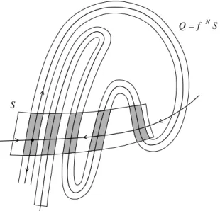
dynamical systems theory was the recognition that very simple,invertible, differentiable dynamical systems can have extremely complex closed invari-ant sets containing an infinite number of periodic and nonperiodic orbits. Smale constructed the most famous example of such a system. It provides an invertible discrete-time dynamical system on the plane possessing an invariant set Λ,whose points are in one-to-one correspondence with all the bi-infinite sequences of two symbols. The invariant set Λ is not a manifold. Moreover,the restriction of the system to this invariant set behaves,in a certain sense,as the symbolic dynamics specified in Example 1.8. That is, how we can verify that it has an infinite number of cycles. Let us explore Smale’s example in some detail.
A
B C
D
A D
(d)
B C
A D
B
C
A D C B
f-1 f
S S
(c) (b)
(a)
FIGURE 1.6. Construction of the horseshoe map.
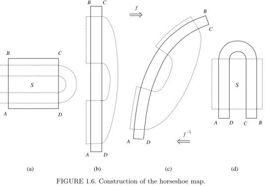
1.3.2 Example 1.9 (Smale horseshoe)
Consider the geometrical construction in Figure 1.6. Take a squareSon the plane (Figure 1.6(a)). Contract it in the horizontal direction and expand it in the vertical direction (Figure 1.6(b)). Fold it in the middle (Figure 1.6(c)) and place it so that it intersects the original square S along two vertical strips (Figure 1.6(d)). This procedure defines a mapf :R2→R2.
The image f(S) of the square S under this transformation resembles a horseshoe. That is why it is called ahorseshoe map. The exact shape of the image f(S) is irrelevant; however,let us assume for simplicity that both the contraction and expansion are linear and that the vertical strips in the intersection are rectangles. The mapf can be made invertible and smooth together with its inverse. The inverse map f−1 transforms the horseshoe f(S) back into the squareS through stages (d)–(a). This inverse transfor-mation maps the dotted squareS shown in Figure 1.6(d) into the dotted horizontal horseshoe in Figure 1.6(a),which we assume intersects the orig-inal squareS along two horizontal rectangles.
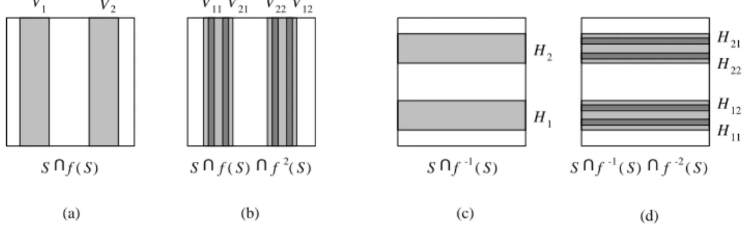
Denote the vertical strips in the intersectionS∩f(S) byV1and V2,
S∩f(S) =V1∪V1
(see Figure 1.7(a)). Now make the most important step: Perform thesecond iterationof the mapf. Under this iteration,the vertical stripsV1,2will be
1.3 Invariant sets 13 2 V 11 12 22 V 1 (b) (a) H1 2 H 21 V V S U V 21 11 22V12
U H H (d) (c) H
S U f-2
H
S f ( )S f-1 f-1( )S
( )
U
S f S U U f2( )S ( )S ( )S
FIGURE 1.7. Vertical and horizontal strips.
four narrow vertical strips: V11, V21, V22,and V12 (see Figure 1.7(b)). We write this as
S∩f(S)∩f2(S) =V11∪V21∪V22∪V12.
Similarly,
S∩f−1(S) =H1∪H2,
whereH1,2 are the horizontal strips shown in Figure 1.7(c),and
S∩f−1(S)∩f−2(S) =H11∪H12∪H22∪H21,
with four narrow horizontal stripsHij(Figure 1.7(d)). Notice thatf(Hi) =
Vi, i= 1,2,as well asf2(Hij) =Vij, i, j= 1,2 (Figure 1.8).
H
f H
(a) (b) (c)
H
H f H
f H 21 22 12 11 f ( ) ( ) 12
( ) 22
f H21
V21 V12 11
V V22
( )
f H11
FIGURE 1.8. Transformationf2(Hij) =Vij, i, j= 1,2.
Iterating the mapf further,we obtain 2k vertical strips in the
intersec-tionS∩fk(S), k= 1,2, . . .. Similarly,iteration off−1gives 2k horizontal
strips in the intersectionS∩f−k(S), k= 1,2, . . ..
Most points leave the squareSunder iteration off orf−1. Forget about
(b) (a)
S f ( )S UU f ( )
S
U
S U f( )S
-1
f ( )S f -2( )S U f-1( )S U 2
FIGURE 1.9. Location of the invariant set.
that remain in the squareS under all iterations off andf−1:
Λ ={x∈S:fk(x)∈S, for allk∈Z}.
Clearly,if the set Λ is nonempty,it is aninvariant setof the discrete-time dynamical system defined byf. This set can be alternatively presented as an infinite intersection,
Λ =· · · ∩f−k(S)∩ · · · ∩f−2(S)∩f−1(S)∩S∩f(S)∩f2(S)∩ · · ·fk(S)∩ · · ·
(any pointx∈Λ must belong to each of the involved sets). It is clear from this representation that the set Λ has a peculiar shape. Indeed,it should be located within
f−1(S)∩S∩f(S),
which is formed byfoursmall squares (see Figure 1.9(a)). Furthermore,it should be located inside
f−2(S)∩f−1(S)∩S∩f(S)∩f2(S),
which is the union ofsixteensmaller squares (Figure 1.9(b)),and so forth. In the limit,we obtain aCantor(fractal)set.
Lemma 1.1 There is a one-to-one correspondence h : Λ → Ω2, between
points ofΛ and all bi-infinite sequences of two symbols.
Proof:
For any pointx∈Λ,define a sequence of two symbols{1,2}
ω={. . . , ω−2, ω−1, ω0, ω1, ω2, . . .}
by the formula
ωk = 1 if f
k(x)∈H1,
2 if fk(x)∈H2, (1.3)
fork= 0,±1,±2, . . .. Here,f0= id,the identity map. Clearly,this formula
defines a maph: Λ→Ω2,which assigns a sequence to each point of the
1.3 Invariant sets 15
To verify that this map is invertible,take a sequenceω∈Ω2,fixm >0,
and consider a setRm(ω) of all pointsx∈S,not necessarily belonging to
Λ,such that
fk(x)∈Hωk,
for −m ≤ k ≤ m−1. For example,if m = 1,the set R1 is one of the four intersectionsVj∩Hk. In general,Rm belongs to the intersection of a
vertical and a horizontal strip. These strips are getting thinner and thinner asm→+∞,approaching in the limit a vertical and a horizontal segment, respectively. Such segments obviously intersect at a single point x with
h(x) = ω. Thus, h : Λ → Ω2 is a one-to-one map. It implies that Λ is
nonempty.✷ Remark:
The maph: Λ→ Ω2 is continuous together with its inverse (a
homeo-morphism) if we use the standard metric (1.1) in S ⊂R2 and the metric
given by (1.2) in Ω2. ♦
Consider now a point x∈ Λ and its corresponding sequence ω =h(x), wherehis the map previously constructed. Next,consider a pointy=f(x), that is,the image ofxunder the horseshoe mapf. Sincey∈Λ by definition, there is a sequence that corresponds to y : θ = h(y). Is there a relation between these sequencesω andθ? As one can easily see from (1.3),such a relation exists and is very simple. Namely,
θk =ωk+1, k∈Z,
sincefk(f(x)) =fk+1(x). In other words,the sequenceθ can be obtained
from the sequenceω by theshift mapσ,defined in Example 1.8:
θ=σ(ω).
Therefore,the restriction off to its invariant set Λ⊂R2 is equivalent to
the shift mapσon the set of sequences Ω2. Let us formulate this result as
the following short lemma.
Lemma 1.2 h(f(x)) =σ(h(x)), for allx∈Λ.
We can write an even shorter one:
f|Λ =h−1◦σ◦h.
Combining Lemmas 1.1 and 1.2 with obvious properties of the shift dy-namics on Ω2,we get a theorem giving a rather complete description of the
behavior of the horseshoe map.
The dynamics on Λ have certain features of “random motion.” Indeed, for any sequence of two symbols we generate “randomly,” thus prescribing the phase point to visit the horizontal stripsH1 andH2in a certain order, there is an orbit showing this feature among those composing Λ.
The next important feature of the horseshoe example is that we can slightly perturb the constructed mapf without qualitative changes to its dynamics. Clearly,Smale’s construction is based on a sufficiently strong contraction/expansion,combined with a folding. Thus,a (smooth) pertur-bation ˜f will have similar vertical and horizontal strips,which are no longer rectangles but curvilinear regions. However,provided the perturbation is sufficiently small (see the next chapter for precise definitions),these strips will shrink tocurves that deviate only slightly from vertical and horizon-tal lines. Thus,the construction can be carried through verbatim,and the perturbed map ˜f will have an invariant set ˜Λ on which the dynamics are completely described by the shift mapσon the sequence space Ω2. As we
will discuss in Chapter 2,this is an example ofstructurally stablebehavior.
Remark:
One can precisely specify the contraction/expansion properties required by the horseshoe map in terms of expandingand contracting cones of the Jacobian matrixfx(see the literature cited in the bibliographical notes in
Appendix 2 to this chapter). ♦
1.3.3 Stability of invariant sets
To represent an observable asymptotic state of a dynamical system,an invariant setS0must be stable; in other words,it should “attract” nearby orbits. Suppose we have a dynamical system {T, X, ϕt} with a complete metric state spaceX. LetS0 be a closed invariant set.
Definition 1.8 An invariant set S0 is calledstable if
(i)for any sufficiently small neighborhood U ⊃S0 there exists a neigh-borhoodV ⊃S0 suchthat ϕtx∈U for allx∈V and all t >0;
(ii) there exists a neighborhood U0 ⊃ S0 suchthat ϕtx → S0 for all
x∈U0, ast→+∞.
IfS0is an equilibrium or a cycle,this definition turns into the standard definition of stable equilibria or cycles. Property (i) of the definition is called
Lyapunov stability. If a setS0is Lyapunov stable,nearby orbits do not leave its neighborhood. Property (ii) is sometimes called asymptotic stability. There are invariant sets that are Lyapunov stable but not asymptotically stable (see Figure 1.10(a)). In contrast,there are invariant sets that are attracting but not Lyapunov stable,since some orbits starting near S0
1.3 Invariant sets 17
S0
0
S
(a) V
U U0
(b)
FIGURE 1.10. (a) Lyapunov versus (b) asymptotic stability.
If x0 is a fixed point of a finite-dimensional,smooth,discrete-time
dy-namical system,then sufficient conditions for its stability can be formulated in terms of the Jacobian matrix evaluated atx0.
Theorem 1.2 Consider a discrete-time dynamical system
x→f(x), x∈Rn,
wheref is a smoothmap. Suppose it has a fixed pointx0, namelyf(x0) = x0, and denote by A the Jacobian matrix of f(x) evaluated at x0, A = fx(x0). Then the fixed point is stable if all eigenvalues µ1, µ2, . . . , µn of A
satisfy|µ|<1.✷
The eigenvalues of a fixed point are usually called multipliers. In the linear case the theorem is obvious from the Jordan normal form. Theorem 1.2,being applied to the N0th iterate fN0 of the map f at any point of
the periodic orbit,also gives a sufficient condition for the stability of an
N0-cycle.
Another important case where we can establish the stability of a fixed point of a discrete-time dynamical system is provided by the following theorem.
Theorem 1.3 (Contraction Mapping Principle) LetX be a complete
metric space withdistance defined byρ. Assume that there is a mapf :X → X that is continuous and that satisfies, for allx, y∈X,
ρ(f(x), f(y))≤λρ(x, y),
withsome0< λ <1. Then the discrete-time dynamical system{Z+, X, fk}
has a stable fixed pointx0∈X. Moreover,fk(x)→x0ask→+∞, starting
from any pointx∈X.✷
restric-tion on the dimension of the spaceX: It can be,for example,an infinite-dimensional function space. Another important difference from Theorem 1.2 is that Theorem 1.3 guarantees the existence and uniqueness of the fixed pointx0,whereas this has to be assumed in Theorem 1.2. Actually,
the map f from Theorem 1.2 is a contraction near x0,provided an
ap-propriate metric (norm) in Rn is introduced. The Contraction Mapping
Principle is a powerful tool: Using this principle,we can prove the Implicit Function Theorem,the Inverse Function Theorem,as well as Theorem 1.4 ahead. We will apply the Contraction Mapping Principle in Chapter 4 to prove the existence,uniqueness,and stability of a closed invariant curve that appears under parameter variation from a fixed point of a generic pla-nar map. Notice also that Theorem 1.3 givesglobal asymptotic stability: Any orbit of{Z+, X, fk}converges to x0.
Finally,let us point out that the invariant set Λ of the horseshoe map is
notstable. However,there are similar invariant fractal sets that are stable. Such objects are calledstrange attractors.
1.4 Differential equations and dynamical systems
The most common way to define a continuous-time dynamical system is by
differential equations. Suppose that the state space of a system isX =Rn
with coordinates (x1, x2, . . . , xn). If the system is defined on a manifold,
these can be considered as local coordinates on it. Very often the law of evolution of the system is given implicitly,in terms of the velocities ˙xi as
functions of the coordinates (x1, x2, . . . , xn):
˙
xi=fi(x1, x2, . . . , xn), i= 1,2, . . . , n,
or in the vector form
˙
x=f(x), (1.4) where the vector-valued functionf :Rn →Rnis supposed to be sufficiently
differentiable (smooth). The function in the right-hand side of (1.4) is re-ferred to as a vector field,since it assigns a vector f(x) to each point x. Equation (1.4) represents a system of nautonomous ordinary differential equations,ODEs for short. Let us revisit some of the examples introduced earlier by presenting differential equations governing the evolution of the corresponding systems.
Example 1.1 (revisited)The dynamics of an ideal pendulum are de-scribed by Newton’s second law,
¨
ϕ=−k2sinϕ,
with
k2=g
1.4 Differential equations and dynamical systems 19
wherelis the pendulum length,andgis the gravity acceleration constant. If we introduceψ= ˙ϕ,so that (ϕ, ψ) represents a point in the state space
X =S1×R1,the above differential equation can be rewritten in the form
of equation (1.4):
˙
ϕ = ψ,
˙
ψ = −k2sinϕ. (1.5)
Here x= ϕ ψ , while f ϕ ψ = ψ −k2sinϕ
.✸
Example 1.2 (revisited)The behavior of an isolated energy-conserving mechanical system withsdegrees of freedom is determined by 2s Hamilto-nian equations:
˙
qi= ∂H
∂pi, p˙i=−
∂H
∂qi, (1.6)
for i = 1,2, . . . , s. Here the scalar function H = H(q, p) is the Hamilton function. The equations of motion of the pendulum (1.5) are Hamiltonian equations with (q, p) = (ϕ, ψ) and
H(ϕ, ψ) = ψ
2
2 +k
2cosϕ. ✸
Example 1.3 (revisited)The behavior of a quantum system with two states having different energies can be described between “observations” by theHeisenberg equation,
idψ
dt =Hψ,
wherei2=−1,
ψ=
a1 a2
, ai∈C1.
The symmetric real matrix
H =
E0 −A
−A E0
, E0, A >0,
is the Hamiltonian matrix of the system,andis Plank’s constant divided
by 2π. The Heisenberg equation can be written as the following system of two linearcomplex equations for the amplitudes
˙
a1 = i1(E0a1−Aa2),
˙
a2 = i1(−Aa1+E0a2).✸
Example 1.4(revisited)As an example of a chemical system,let us consider theBrusselator[Lefever & Prigogine 1968]. This hypothetical sys-tem is composed of substances that react through the following irreversible stages:
A k1
−→ X
B+X k2
−→ Y +D
2X+Y k3
−→ 3X
X k4
−→ E.
Here capital letters denote reagents,while the constantskiover the arrows
indicate the corresponding reaction rates. The substancesDandE do not re-enter the reaction,whileAandBare assumed to remain constant. Thus, thelaw of mass actiongives the following system of two nonlinear equations for the concentrations [X] and [Y]:
d[X]
dt = k1[A]−k2[B][X]−k4[X] +k3[X] 2[Y],
d[Y]
dt = k2[B][X]−k3[X] 2[Y].
Linear scaling of the variables and time yields theBrusselator equations, ˙
x = a−(b+ 1)x+x2y,
˙
y = bx−x2y. ✸ (1.8)
Example 1.5 (revisited)One of the earliest models of ecosystems was the system of two nonlinear differential equations proposed by Volterra [1931]:
˙
N1 = αN1−βN1N2,
˙
N2 = −γN2+δN1N2. (1.9)
HereN1andN2are the numbers of prey and predators,respectively,in an ecological community,αis the prey growth rate,γis the predator mortality, whileβ andδdescribe the predators’ efficiency of consumption of the prey.
✸
Under very general conditions,solutions of ODEs define smooth conti-nuous-time dynamical systems. Few types of differential equations can be solved analytically (in terms of elementary functions). However,for smooth right-hand sides,the solutions are guaranteed to exist according to the following theorem. This theorem can be found in any textbook on ordinary differential equations. We formulate it without proof.
Theorem 1.4(Existence, uniqueness, and smooth dependence)
Consider a system of ordinary differential equations
˙
1.4 Differential equations and dynamical systems 21
wheref :Rn→Rn is smoothin an open region U ⊂Rn. Then there is a
unique function x=x(t, x0),x:R1×Rn →Rn, that is smooth in (t, x),
and satisfies, for eachx0∈U, the following conditions: (i)x(0, x0) =x0;
(ii) there is an interval J = (−δ1, δ2), where δ1,2 = δ1,2(x0)>0, such
that, for allt∈ J,
y(t) =x(t, x0)∈U,
and
˙
y(t) =f(y(t)).✷
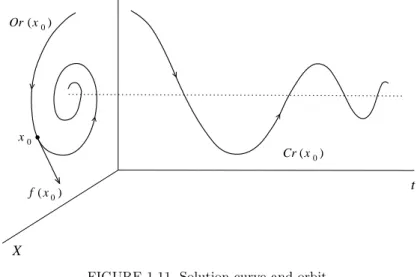
The degree of smoothness ofx(t, x0) with respect tox0 in Theorem 1.4 is the same as that of f as a function of x. The function x = x(t, x0), considered as a function of time t,is called a solution starting at x0. It defines,for eachx0∈U,two objects: asolution curve
Cr(x0) ={(t, x) :x=x(t, x0), t∈ J } ⊂R1×Rn
and anorbit,which is the projection ofCr(x0) onto the state space,
Or(x0) ={x:x=x(t, x0), t∈ J } ⊂Rn
(see Figure 1.11). Both curves are parametrized by timetand oriented by the direction of time advance. A nonzero vector f(x0) is tangent to the orbitOr(x0) atx0. There is auniqueorbit passing through a pointx0∈U. Under the conditions of the theorem,the orbit either leavesU att=−δ1
(and/or t = δ2),or stays in U forever; in the latter case,we can take
J = (−∞,+∞).
Now we can define the evolution operatorϕt:Rn →Rn by the formula
ϕtx0=x(t, x0),
which assigns tox0 a point on the orbit throughx0 that is passedt time units later. Obviously,{R1,Rn, ϕt} is a continuous-time dynamical system
(check!). This system isinvertible. Each evolution operatorϕtis defined for
x∈U andt∈ J,whereJ depends onx0 and is smooth inx. In practice, the evolution operatorϕt corresponding to a smooth system of ODEs can
be found numerically on fixed time intervals to within desired accuracy. One of the standard ODE solvers can be used to accomplish this.
0 x
t
( )
f
X Or x0
x0
Cr x0
( )
( )
FIGURE 1.11. Solution curve and orbit.
equilibria of a system defined by (1.4) are zeros of the vector field given by its right-hand side:
f(x) = 0. (1.10)
Clearly,iff(x0) = 0,then ϕtx0 = x0 for all t ∈ R1. The stability of an
equilibrium can also be detected without solving the system. For example, sufficient conditions for an equilibriumx0 to be stable are provided by the
following classical theorem.
Theorem 1.5 (Lyapunov [1892]) Consider a dynamical system defined
by
˙
x=f(x), x∈Rn,
wheref is smooth. Suppose that it has an equilibriumx0 (i.e.,f(x0) = 0),
and denote byA the Jacobian matrix off(x) evaluated at the equilibrium,
A=fx(x0). Thenx0 is stable if all eigenvaluesλ1, λ2, . . . , λn of A satisfy
Reλ <0.✷
Recall that the eigenvalues are roots of thecharacteristic equation
det(A−λI) = 0,
whereI is then×nidentity matrix.
The theorem can easily be proved for a linear system
˙
x=Ax, x∈Rn,
1.5 Poincar´e maps 23
0
x
FIGURE 1.12. Lyapunov function.
whose level surfacesL(x) =L0 surround the origin and are such that the vector field points strictly inside each level surface,sufficiently close to the equilibriumx0 (see Figure 1.12). Actually,the Lyapunov functionL(x) is
the same for both linear and nonlinear systems and is fully determined by the Jacobian matrixA. The details can be found in any standard text on differential equations (see the bibliographical notes in Appendix 2). Note also that the theorem can also be derived from Theorem 1.2 (see Exercise 7).
Unfortunately,in general it is impossible to tell by looking at the right-hand side of (1.4),whether this system has cycles (periodic solutions). Later on in the book we will formulate some efficient methods to prove the appearance of cycles under small perturbation of the system (e.g.,by variation of parameters on which the system depends).
If the system has a smooth invariant manifoldM,then its defining vector field f(x) is tangent to M at any point x∈ M,where f(x) = 0. For an (n−1)-dimensional smooth manifoldM ⊂Rn,which is locally defined by g(x) = 0 for some scalar functiong:Rn→R1,the invariance means
∇g(x), f(x)= 0.
Here∇g(x) denotes thegradient
∇g(x) =
∂g(x)
∂x1 , ∂g(x)
∂x2 , . . . , ∂g(x)
∂xn
T
,
which is orthogonal toM atx.