Stability of a Two-Sublattice Spin-Glass Model
Carlos S. O. Yokoi
Instituto de F´ısica, Universidade de S˜ao Paulo, Caixa Postal 66318, 05315-970 S˜ao Paulo, SP, Brazil
and Francisco A. da Costa
Departamento de F´ısica Te´orica e Experimental, Universidade Federal do Rio Grande do Norte,
Caixa Postal 1641, 59072-970 Natal, RN, Brazil
Received on 6 October, 2003
We study the stability of the replica-symmetric solution of a two-sublattice infinite-range spin-glass model, which can describe the transition from an antiferromagnetic to a spin-glass state. The eigenvalues associated with replica-symmetric perturbations are in general complex. The natural generalization of the usual stability condition is to require the real part of these eigenvalues to be positive. The necessary and sufficient conditions for all the roots of the secular equation to have positive real parts is given by the Hurwitz criterion. The generalized stability condition allows a consistent analysis of the phase diagram within the replica-symmetric approximation.
1
Introduction
The infinite-range Sherrington-Kirkpatrick (SK) model [1] for a spin glass has attracted considerable attention over the past decades [2, 3, 4]. These investigations have re-vealed highly non-trivial properties such as the instability of the symmetric (RS) solution [5] and the replica-symmetry-breaking scheme to produce a stable solution [6-9]. Most studies have concentrated on situations where the exchange distributions are either symmetric or with an ad-ditional ferromagnetic interaction. More recently a two-sublattice version of the SK model was introduced [10-13] to allow for antiferromagnetic interactions between differ-ent sublattices. Such extension is quite natural in view of the existence of many experimental systems such as FexMg1−xCl2[14-16] and FexMn1−xTiO3[17, 18], which exhibit a transition from an Ising antiferromagnetic into an Ising spin glass state for a certain range ofxvalues. In con-trast to the standard SK model, in the two-sublattice SK model with antiferromagnetic intersublattice interactions, the ordered (antiferromagnetic) phase extends to finite fields and the de Almeida-Thouless instability line [5] has dis-tinct branches in the paramagnetic and antiferromagnetic phases, which do not meet at a first-order transition [10-13]. Experimental determination of the field-temperature phase diagram in FexMn1−xTiO3, as well as the de Almeida-Thouless instability line [19], are in qualitative agreement with mean-field results [13].
In the previous studies of this model the stability of the RS solution against transversal fluctuations, i.e., outside the RS space, has already been investigated [10-13], and the stability against longitudinal fluctuations, i.e., inside the RS space, was also briefly considered [12]. The stability of the
RS solution against transversal fluctuations is important to establish whether replica symmetry breaking is necessary. The stability against longitudinal fluctuations, however, is also necessary to ensure the validity of RS solution. For cer-tain parameter values of the two-sublattice SK model there may be up to three RS solutions, all of them stable against transversal fluctuations. In such a situation the analysis of the stability against longitudinal fluctuations is important for a consistent study of the phase diagram by eliminating un-stable solutions.
In this work we remedy the lack of such investigation by a detailed numerical and analytical study of the eigenvalues associated with longitudinal fluctuations. Surprisingly, these eigenvalues are in general complex. It is natural to assume that stability condition should require the real part of these eigenvalues to be positive. The necessary and sufficient con-dition for all the roots of the secular equation to have pos-itive real parts is given by the Hurwitz criterion. We show that this generalized stability condition allows a consistent study of the phase diagram within the RS approximation.
2
The model
We consider a system of2NIsing spinsSi=±1located at the sites of two identical sublatticesAandB. The interac-tions are described by the Hamiltonian
H=− X
i∈A,j∈B
JijSiSj−
X
(ij)∈A J′
ijSiSj
− X
(ij)∈B J′
ijSiSj−H
X
i
where the first sum is over all distinct pairs of spins belong-ing to different sublattices, the second and third ones refer to all distinct pairs of spins belonging to the same sublattices, and the last sum is over all spins in the two sublattices. Jij is the exchange interaction between spins in different sub-lattices,J′
ijis the exchange interaction between spins in the same sublattice, andH is the applied magnetic field. The exchange interactions are independent, quenched, Gaussian random variables with mean values
hJijiJ= J0 N, hJ
′ ijiJ=
J′ 0
N, (2) and variances
hJij2iJ− hJiji2J= J2
N, hJ ′2
ijiJ− hJij′ i2J = J′2
N . (3)
The mean intrasublattice interactions will always assumed to be ferromagnetic (J′
0>0), whereas the mean intersublat-tice interactions may be ferromagnetic (J0 >0) or antifer-romagnetic (J0<0).
The standard approach to compute the quenched average is to introducennon-interacting replicasα= 1,2, . . . , nof the system, calculate the annealed averages and then take the limitn → 0[2, 4]. In this replica method the free energy per spinfis given by
f = 1 2β nlim→0
1
nφ, φ=−Nlim→∞
1
N ln hZ n
iJ, (4)
whereβ = 1/kBT andZn is the partition function ofn replicas of the system. Performing the average ofZn over the random couplings we find
⌋
hZniJ = Tr exp−N
(
−β
2J2n
2 +βJ
′ 0
n N −
β2J′2n
2
³
1−Nn´−βHX α
(mαA+mαB)
−βJ0X
α
mαAmαB− βJ′ 0 2 X α h
(mαA) 2
+ (mαB) 2i
−β2J2X (αβ)
qαβA qαβB
−β
2J′2
2
X
(αβ)
·³
qAαβ´2+³qαβB ´2
¸
, (5)
where(αβ)denotes distinct pairs of replicas and we have introduced the sublattice magnetization and sublattice overlap function of the replicas,
mαX=
1
N
X
i∈X
Siα, q αβ
X =
1
N
X
i∈X SiαS
β
i, (X =A, B). (6)
The trace over the spin variables in (5) can be performed by taking into account the constraints (6) by means of the identities
1 =
Z ∞
−∞ dmα
X
Z i∞
−i∞ N dλα
X
2πi exp
"
−N λα X Ã mα X− 1 N X
i∈X Sα
i
!#
(X=A, B), (7)
and
1 =
Z ∞
−∞ dqαβX
Z i∞
−i∞ N dλαβX
2πi exp
"
−N λαβX
Ã
qαβX −N1 X
i∈X SαiS
β i
!#
(X=A, B). (8)
We then obtain
hZniJ =
Y
α
Z ∞
−∞ dmαA
Z i∞
−i∞ N dλα
A
2πi
Z ∞
−∞ dmαB
Z i∞
−i∞ N dλα
B
2πi
Y
(αβ)
Z ∞
−∞ dqAαβ
Z i∞
−i∞ N dλαβA
2πi
×
Z ∞
−∞ dqBαβ
Z i∞
−i∞ N dλαβB
2πi exp
h
−N φ(mαA, mαB, q αβ A , q
αβ B ;λ
α A, λαB, λ
αβ A , λ
αβ B )
i
, (9)
where
φ = −β
2J2n
2 +βJ
′ 0
n N −
β2J′2n
2
³
1− n
N
´
−βHX
α
(mα
A+mαB)−βJ0
X
α mα
AmαB
−βJ ′ 0 2 X α h
(mαA) 2
+ (mαB) 2i
−β2J2X (αβ)
qAαβqBαβ−β
2J′2
2
X
(αβ)
·³
qAαβ´2+³qBαβ´2
¸
+X
α
(λαAmαA+λαBmαB) +
X
(αβ)
³
withHAandHBdenoting the “effective sublattice Hamiltonians”,
HX =
X
α
λαXSα+
X
(αβ)
λαβX SαSβ (X =A, B). (11)
In the limit of largeNthe integrations over theλvariables in (9) can be performed by the saddle-point method. The saddle point is given by
mαX =
TrSαexpH X Tr expHX
, qXαβ=TrS
αSβexpH X Tr expHX
, (X =A, B). (12) These equations determineλvariables in terms ofmandqvariables. The remaining integrations over themandqvariables in (9) can be performed by the Laplace method in the limit of largeN. The stationary-point equations are given by
λα
X =βH+βJ ′
0mαX+βJ0mαX, λαβX =β2J ′2qαβ
X +β2J2q αβ
X , (X =A, B), (13)
whereX is the sublattice complementary toX, i.e., ifX =AthenX =B, and vice versa. Substituting these results in the expression ofφgiven by Eq. (10) we find
φ = −β
2n
2 (J
2+J′2) +βJ0X α
mαAmαB+ βJ′
0
2
X
α
h
(mαA) 2
+ (mαB) 2i
+β2J2X (αβ)
qAαβqBαβ
+β
2J′2
2
X
(αβ)
·³
qαβA ´2+³qBαβ´2
¸
−lnTr expHA−lnTr expHB, (14)
where we have discarded terms that vanish in the limit of largeN. Analogously, the effective sublattice Hamiltonians (11) become
HX=β
X
α
¡
H+J′
0mαX+J0mαX
¢
Sα+β2X (αβ)
³
J′2qαβ X +J2q
αβ X
´
SαSβ, (X=A, B). (15)
To evaluate the general expressions obtained thus far it is necessary to impose some structure on mand qvariables. The simplest assumption corresponds to the RS solution[2, 4] obtained by assuming order parameters independent of replica indices,
mαX=mX, qαβX =qX, (X =A, B). (16) Proceeding in the usual way [2, 4], one finds that the saddle-point equations (12) and stationary-point equations (13) give the equations of state
mX=htanhHXi, qX =tanh2HX®, (X =A, B), (17) where
HX=β
µ
H+J′
0mX+J0mX+
q
J′2q
X+J2qXx
, (X=A, B), (18) and the brackets without subscripth· · · idenote Gaussian averages,
h· · · i=
Z ∞
−∞ dx
√ 2πe
−x2/2
(· · ·). (19)
Analogously, the free energy per spin (4) becomes
f = −βJ
2
4 (1−qA) (1−qB)−
βJ′2
8
h
(1−qA)2+ (1−qB)2
i
+J0
2 mAmB+
J′ 0
4
¡
m2A+m2B
¢
−21β hln 2 coshHAi − 1
2βhln 2 coshHBi. (20)
⌈
3
The stability of replica-symmetric
solution
The validity of the RS solution (17) rests on the applicabil-ity of Laplace method used to perform the integrations over
respect to the m andqvariables are all positive. We can equivalently considerφas a function ofλvariables, related tomandqvariables by means of Eq. (12). We will follow
the latter approach because it leads to simpler calculations. The Hessian is a[n(n+ 1)/2]×[n(n+ 1)/2]matrix whose elements are2×2matrices given by
⌋
Gαβ=
µ
GαβAA GαβAB GαβBA G
αβ BB
,Gα(βγ)=
Ã
GαAA(βγ) GαAB(βγ) GαBA(βγ) GαBB(βγ)
!
,G(αβ)(γδ)=
Ã
G(AAαβ)(γδ) G(ABαβ)(γδ) G(BAαβ)(γδ) G(BBαβ)(γδ)
!
, (21)
where
GαβXY = ∂2φ ∂λα
X∂λ β Y
, GαXY(βγ)=
∂2φ ∂λα
X∂λ (βγ) Y
, G(XYαβ)(γδ)= ∂2φ
∂λαβX∂λγδY (X, Y =A, B). (22) At the stationary point of the RS solution (17) there are seven different types of2×2elements of the Hessian matrix. We denote these elements by [5]
Gαα=A, Gαβ=B, Gα(αβ)=C, G(αβ)α=Ce, Gα(βγ)=D,
G(αβ)γ=De, G(αβ)(αβ)=P, G(αβ)(αγ)=Q, G(αβ)(γδ)=R, (23)
⌈
where the indicesα,β,γandδare all distinct and the tilde denotes the transpose of the matrix. We do not quote the lengthy expressions for these elements because only their linear combinations are needed in the calculation of the eigenvalues.
The eigenvalues of the Hessian matrix can now be de-termined by finding the eigenvectors that divide the space into orthogonal subspaces closed to the permutation oper-ation. The procedure are analogous to the case of the SK model [5] except that now the elements of the Hessian
ma-trix are 2×2matrices (23). These eigenvectors are [20]: n(n−3)transversal or replicon eigenvectors depending on two replica indices,4(n−1)anomalous eigenvalues depend-ing on a sdepend-ingle replica index, and 4 longitudinal eigenvectors independent of replica indices.
The eigenvalues associated with the transversal eigen-vectors are found to be the eigenvalues of the2×2matrix
T=P−2Q+R, (24)
with elements
⌋
T11 = (1−2qA+rA)−(βJ′)2(1−2qA+rA)2, (25) T12 = T21=−(βJ)2(1−2q
A+rA)(1−2qB+rB), (26)
T22 = (1−2qB+rB)−(βJ′)2(1−2qB+rB)2, (27) where
tX=tanh3HX®, rX=tanh4HX®, (X=A, B). (28) The necessary and sufficient condition for all the eigenvalues to be positive are
T11+T22>0 and T11T22−T2
12>0, (29)
which are equivalent to the conditions
T1 = 2−(βJ′
)2(1−2q
A+rA)−(βJ′)2(1−2qB+rB)>0, (30) T2 = [1−(βJ′
)2(1−2qA+rA)][1−(βJ′)2(1−2qB+rB)]
−(βJ)4(1−2qA+rA)(1−2qB+rB)>0, (31)
in agreement with previous studies [10, 13]. A RS solution satisfying these conditions will be called transversally (T) stable, and T unstable otherwise.
The eigenvalues associated with anomalous and longitudinal eigenvectors are the same in the limitn→0. They are found to be the eigenvalues of the4×4matrix
L=
µ A
−B D−C
2Ce −2De P−4Q+3R
where
L11 = (1−qA)−βJ0′(1−qA)2+ 2(βJ′)2(tA−mA)2, (33) L22 = (1−qB)−βJ0′(1−qB)2+ 2(βJ′)2(tB−mB)2, (34) L12 = L21=−βJ0(1−qA)(1−qB) + 2(βJ)2(tA−mA)(tB−mB), (35) L13 = −12L31= (tA−mA)[1−βJ0′(1−qA)−(βJ′)2(1−4qA+ 3rA)], (36) L24 = −12L42= (tB−mB)[1−βJ0′(1−qB)−(βJ′)2(1−4qB+ 3rB)], (37) L14 = −12L41=−βJ0(tB−mB)(1−qA)−(βJ)2(tA−mA)(1−4qB+ 3rB), (38) L23 = −12L32=−βJ0(tA−mA)(1−qB)−(βJ)2(tB−mB)(1−4qA+ 3rA), (39) L33 = (1−4qA+ 3rA)[1−(βJ′)2(1−4qA+ 3rA)] + 2βJ0′(tA−mA)2, (40) L44 = (1−4qB+ 3rB)[1−(βJ′)2(1−4qB+ 3rB)] + 2βJ0′(tB−mB)2, (41) L34 = L43=−(βJ)2(1−4qA+ 3rA)(1−4qB+ 3rB) + 2βJ0(tA−mA)(tB−mB). (42)
⌈
The characteristic equation has the form
λ4−a1λ3+a2λ2−a3λ+a4= 0, (43) where the coefficientsanaren-th order traces of the matrix L. A numerical study of equation (43) shows that the eigen-values are complex for some eigen-values of the parameters of the model, in contrast with one-sublattice SK model in which the anomalous and longitudinal eigenvalues never become complex [5]. Even though the Hessian matrix (21) forn >1
is real and symmetric, in the limitn →0there is no guar-antee that the eigenvalues will be real. In fact, complex lon-gitudinal and anomalous eigenvalues also arise in the spin 1 one-sublattice infinite-range spin-glass model with crystal-field anisotropy [21, 22]. In general, therefore, the stability condition should require the real part of the eigenvalues to be positive. According to the Hurwitz criterion [23], the nec-essary and sufficient condition for all the roots of equation (43) to have positive real parts are
⌋
D1 = a1>0, D2=
¯ ¯ ¯
¯ a11 a3a2
¯ ¯ ¯
¯=a1a2−a3>0, (44)
D3 =
¯ ¯ ¯ ¯ ¯ ¯
a1 a3 0
1 a2 a4
0 a1 a3
¯ ¯ ¯ ¯ ¯
¯=a3D2−a
2
1a4>0, D4=
¯ ¯ ¯ ¯ ¯ ¯ ¯ ¯
a1 a3 0 0
1 a2 a4 0
0 a1 a3 0
0 1 a2 a4
¯ ¯ ¯ ¯ ¯ ¯ ¯ ¯
=a4D3>0. (45)
⌈
These condition are equivalent to the following four condi-tions:
L1 = a1>0, (46) L2 = D2=a1a2−a3>0, (47) L3 = D3=a1a2a3−a32−a4a21>0, (48) L4 = a4>0. (49)
A RS solution satisfying these conditions will be called lon-gitudinally (L) stable, and L unstable otherwise.
4
Results of the stability analysis
In this section we present the results of the stability analysis of the RS solution for different values of the parameters of the model. Since the Hamiltonian (1) is invariant under the simultaneous transformations
H→ −H, Si→ −Si, (50)
4.1
Zero applied field
4.1.1 Ferromagnetic intersublattice interaction
In zero applied field (H = 0) and ferromagnetic intersub-lattice interactions (J0>0) the solutions of the set of equa-tions (17) are of the form
mA=mB =m, qA=qB =q. (51) Three types of solutions are possible:
• Paramagnetic (P) solution:m= 0, q= 0.
• Spin Glass (SG) solution:q >0, m= 0.
• Ferromagnetic (F) solution:q >0, m >0.
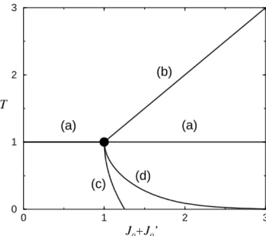
Fig. 1 shows the lines delimiting the regions where different types of solutions can be found in the plane of temperature versusJ0+J′
0.
The P solution is always possible. However it is L stable only above the line (b) and the left portion of line (a), and T stable above line (a). The L instability of P solution occurs due to the violation of the condition (49), which is given in the case of P solution by
L4= [1−β2(J′2
−J2)][1−β2(J′2+J2)]
[1−β(J′
0−J0)][1−β(J ′
0+J0)]>0. (52) For(J0+J′
0)/
√
J2+J′2 ≤ 1/2, the second factor of in (52) becomes negative below line (a). Thus the left portion of line (a) is determined by
β2(J′2+J2) = 1. (53) On the other hand, for(J0+J′
0)/
√
J2+J′2 > 1/2 the fourth factor in (52) becomes negative below line (b). Thus the equation for line (b) is
β(J′
0+J0) = 1. (54)
0 1 2 3
J0+J0’
0 1 2 3
T
(a)
(b)
(c) (d) (a)
Figure 1. Regions of the zero-field phase diagram where different types of solution are possible. For ferromagnetic intersublattice in-teraction (J0>0), the P solution is L stable above line (b) and the left portion of line (a), the F solution between lines (b) and (c), and SG solution between the left portion of line (a) and line (c). The P solution is T stable above line (a), the F solution between lines (b) and (d). The SG solution is T unstable between the left side of line (a) and line (c), and F solution between lines (c) and (d). For antiferromagnetic intersublattice interaction (J0 <0) the F solu-tion is replaced by AF solusolu-tion and the label of horizontal axis by
−J0+J0′. The temperature and energy units in the axis are such that√J2+J′2= 1
andkB = 1.
The T instability of the P solution is due to the violation of the condition (31), which is given in the case of P solution by
T2= [1−β2(J′2
−J2)][1−β2(J′2+J2)]>0. (55) The second factor in (55) becomes negative below line (a) for all values of J0 +J′
0. Thus line (a) is given by equation (53) for all J0 +J′
0. The T and L instabilities of the P solution occur simultaneously on the line (a) for
(J0+J′ 0)/
√
J2+J′2≤1/2.
The SG solution is possible only below line (a). It is T unstable throughout this region and L stable to the left of line (c). The L instability of the SG solution occurs due to the violation of the condition (49), which is given in the case of SG solution by
⌋
L4= (1−q)2(1−4q+ 3r)2 [1−β2(J′2
−J2)(1−4q+ 3r)][1−β2(J′2+J2)(1
−4q+ 3r)] ×[1−β(J′
0−J0)(1−q)][1−β(J ′
0+J0)(1−q)]>0. (56) For(J0+J′
0)/
√
J2+J′2>1/2the last factor in (56) becomes negative to the left of line (c). Thus the equation determining line (c) is
β(J′
0+J0)(1−q) = 1. (57)
The F solution is possible only between lines (b) and (c). It is L stable throughout this region but T stable only above line (d). The T instability of the F solution occurs due to the violation of the condition (31), which is given in the case of F solution by
T2= [1−β2(J′2
−J2)(1−2q+ 3r)][1−β2(J′2+J2)(1
For(J0+J′ 0)/
√
J2+J′2 >1/2the second factor in (58) becomes negative below line (d). Thus line (d) is described by equation
β2(J′2+J2)(1−2q+ 3r) = 1. (59) Rejecting solutions that are L unstable, we conclude that the P phase is located above lines (b) and left portion of line (a), the SG phase between the left portion of line (a) and line (c), and finally the F phase between lines (b) and (c). The SG phase, and the F phase between lines (c) and (d), are T unstable, indicating the need for a replica-symmetry-breaking solution in this region. The transition line (c) will change to a vertical line if such a solution is considered [24]. We mention that, as should be expected, in the caseJ0 = 0
andJ = 0, orJ′
0 = 0andJ′ = 0, these results reduce to those of one-sublattice SK model [2, 4].
4.1.2 Antiferromagnetic intersublattice interaction
The Hamiltonian (1) in zero applied field (H = 0) is invari-ant under simultaneous transformations
J0−→ −J0, Si−→ −Si (i∈B). (60) In fact, we can check explicitly that all the expressions for the RS solution, including those of stability conditions, are invariant under simultaneous transformations
J0−→ −J0, mB−→ −mB. (61) Thus the case of antiferromagnetic intersublattice interac-tion J0 < 0 is completely equivalent to the case of ferro-magnetic intersublattice interaction −J0 > 0by replacing mBby−mB. This means that the F solution is replaced by the antiferromagnetic (AF) solution
mA=−mB=m, qA=qB =q. (62) The results displayed in Fig. 1 remains valid, with J0 re-placed by−J0and F solution by AF solution.
4.2
Non-zero applied field
4.2.1 Ferromagnetic intersublattice interaction
In non-zero applied field (H >0) and ferromagnetic inter-sublattice interactions (J0 >0), only the paramagnetic (P) solution is possible for the set of equations (17), which are of the form
mA=mB=m >0, qA=qB =q >0. (63)
0.0 0.2 0.4 0.6 0.8 1.0 H
0.0 0.2 0.4 0.6 0.8 1.0 1.2
T AT
Figure 2. Region of stability in the presence of a field for the case of ferromagnetic intersublattice interaction (J0 < 0). The values of parameters are J′/J = 1, J′
0/J0 = 1 and (J0 +
J′
0)/ √
J2+J′2 = 1/2
. There is only the P solution which is always L stable but becomes T unstable below the de Almeida-Thouless line AT. The temperature and field units in the axis are such that√J2+J′2= 1
andkB= 1.
This solution is always L stable, but becomes T unstable for low temperatures due to the violation of the condition (31), which in this case is also given by Eq. (58). The instability line is given by Eq. (59), illustrated in Fig. 2 for the case J′/J = 1,J′
0/J0 = 1/2and(J0+J0′)/
√
J2+J′2 = 2. As should be expected, in the caseJ0 = 0andJ = 0, or J′
0= 0andJ′ = 0, these results reduce to the de Almeida-Thouless line of one-sublattice SK model[5].
4.2.2 Antiferromagnetic intersublattice interaction
In non-zero applied field (H >0) and antiferromagnetic in-tersublattice interactions (J0<0), two types of solutions to the set of equations (17) are possible:
• Paramagnetic (P) solution: mA = mB = m >
0, qA=qB =q >0.
• Antiferromagnetic (AF) solution: mA 6=mB, qA 6= qB.
For(−J0+J′ 0)/
√
J2+J′2 ≤ 1/2only P solution is possible. This solution is always L stable but becomes T un-stable at low temperatures due to the to the violation of the condition (31), which in this case it is also given by (58). The instability line is given by Eq. (59).
For(−J0 +J′ 0)/
√
J2+J′2 > 1/2, AF solution also becomes possible. Fig. 3 shows the lines delimiting the re-gions of existence and stability of each type of solution for
−J′
0/J0 = 1/2. The P solution becomes L unstable below line (a) due to the violation of the condition (49). In the case of P solution this condition is given by
⌋
L4 = [(1−q)(1−4q+ 3r) + 2(t−m)2]2©[1−β(J′
0+J0)(1−q)][1−β(J ′2
−J2) ×(1−4q+ 3r)] + 2β3(J′
0+J0)(J ′2
−J2)(t−m)2ª{[1−β(J′
0−J0)(1−q)]
×[1−β(J′2+J2)(1
−4q+ 3r)] + 2β3(J′
0−J0)(J
′2+J2)(t
The first factor in (64) becomes negative inside line (a). Therefore the equation determining line (a) is
[1−β(J′
0−J0)(1−q)][1−β(J ′2
−J2)(1−4q+ 3r)] + 2β3(J′
0−J0)(J ′2
−J2)(t−m)2= 0, (65)
⌈
0.0 0.5 1.0 1.5 2.0
H 0.0
0.5 1.0 1.5 2.0 2.5
T
(a)
(b)
(c)
(b)
Figure 3. Regions of stability and existence of different solu-tions in the temperature versus field phase diagram for the case of antiferromagnetic intersublattice interaction (J0<0). The val-ues of parameters areJ′/J = 1,
−J0′/J0 = 1/2and(−J0+
J′
0)/ √
J2+J′2 = 2. The P solution is L stable outside line (a) and T stable above line (b). The AF solution is possible only inside line (a) and it is always L stable, but becomes T unstable below line (c). The temperature and field units in the axis are such that √
J2+J′2= 1
andkB= 1.
which is in agreement with previous study [12]. The P so-lution is T unstable below line (b). This instability occurs due to the violation of condition (31), given in this case by Eq. (58), caused by the second factor. Therefore the line (b) is determined by equation (59). The AF solution is possible only inside line (a). It is L stable throughout this region and T unstable below line (c). This instability is due to the viola-tion of condiviola-tion (31). Therefore line (c) obeys the equaviola-tion
[1−(βJ′
)2(1−2qA+rA)][1−(βJ′)2(1−2qB+rB)]
= (βJ)4(1−2q
A+rA)(1−2qB+rB). (66) Rejecting solutions that are L unstable, we conclude that P phase exists outside and AF phase inside line (a). The P solution becomes T unstable below line (b) and AF solu-tion below line (c), which meet smoothly on the line (a). In the region below lines (b) and (c) it is necessary to consider replica symmetry breaking solution, which will presumably change line (a) in this region.
For sufficiently large values of the ratio −J′ 0/J0 the model can exhibit first-order transition from AF phase to the P phase [12]. As an example, we consider the case
−J′
0/J0 = 5shown in Fig. 4. The P solution is L stable inside line (a) given by Eq. (65), and T stable above line (b) given by Eq. (66). There is one AF solution inside line (a) and two distinct AF solutions between lines (a) and (d), as
illustrated in Figs. 5(a) and 5(b) forkBT /
√
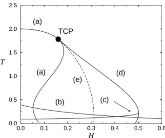
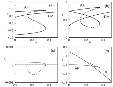
J2+J′2 = 1. One of the AF solutions, corresponding to dotted lines in Fig. 5, is L unstable due to the violation of the condition (49), as shown in Fig. 5(c). The transition between AF phase and P phase is first order, determined by equating the free energies of L stable AF and P phases, as shown in Fig. 5(d). The first-order transition line is shown as dot-ted line in Fig. 4, which ends at the tricritical point TCP. The L stable AF solution becomes T unstable below line (c) due to the violation of condition (31), and it is determined by Eq. (66). We conclude that in Fig. 4 the P phase exists outside and AF phase inside lines (a) and (e), which meet smoothly at the tricritical point TCP. The P phase becomes T unstable below line (b), and AF phase below line (c). Notice that the lines (b) and (c) are discontinuous across first-order transition [12]. It is likely that the first-order transition line will change in this part of phase diagram once the replica-symmetry-breaking solutions are considered for P and AF phases.
0.0 0.1 0.2 0.3 0.4 0.5 0.6
H 0.0
0.5 1.0 1.5 2.0 2.5
T
(a)
(b) TCP
(c) (d) (e)
(a)
Figure 4. Regions of stability and existence of different solu-tions in the temperature versus field phase diagram for the case of antiferromagnetic intersublattice interaction (J0 < 0). The values of parameters areJ′/J = 1,
−J0′/J0 = 5and (−J0 +
J′
0)/ √
J2+J′2 = 2
0.0 0.2 0.4 H −0.001
0 0.001
L4
−0.001
H
0 0.2 0.4 H −1.0
−0.5 0.0 0.5 1.0 1.5
m
0 0.2 0.4 H −1.3
−1.2 −1.1 −1 −0.9
f
0 0.2 0.4 H 0
0.5 1
q
AF
PM PM
(a)
AF
(b)
P
(c) (d)
AF
Figure 5. Field behavior of various quantities for the fixed value of temperaturekBT /
√
J2+J′2= 1
in the phase diagram of Fig. 4. In (a) and (b) the order parameters of the P and AF solution are shown, in (c) the L stability conditionL4of the AF solution, and finally in (d) the free-energy per spin of P and AF solutions. The L unstable AF solution are represented by dotted lines, and corre-sponds to the upper portion of the van der Waals loop in (d). The first-order transition is determined by the intersection of L stable AF and P solutions, as depicted in (d). The temperature and energy units in the axis are such that√J2+J′2= 1
andkB = 1.
5
Conclusions
In this paper we have investigated the stability of the RS symmetric solution of the two-sublattice generalization of the SK infinite-range spin-glass model. We have derived stability conditions for transversal fluctuations in agreement with previous investigations, and we have extended previous study of the stability against longitudinal or anomalous fluc-tuations. The eigenvalues associated with such perturbations are in general complex. We generalized the usual stability condition by requiring the real part of these eigenvalues to be positive. The necessary and sufficient stability conditions were found using the Hurwitz criterion for all the roots of the secular equation to have positive real parts. These con-ditions allowed us to select one RS solution among those that are transversally stable. We believe that the generalized stability condition should also be useful in other spin glass models where eigenvalues associated with longitudinal and anomalous perturbations become complex.
Acknowledgments
The authors acknowledge partial financial support from the Brazilian Government Agencies PROCAD/CAPES and CNPq.
References
[1] D. Sherrington and S. Kirkpatrick, Phys. Rev. Lett. 35, 1792 (1975).
[2] K. Binder and A. P. Young, Rev. Mod. Phys. 58, 801 (1986).
[3] M. M´ezard, G. Parisi, and M. A. Virasoro, Spin Glass Theory
and Beyond (World Scientific, Singapore, 1987).
[4] K. H. Fischer and J. H. Hertz, Spin Glasses (Cambridge Uni-versity Press, Cambridge, 1991).
[5] J. R. L. de Almeida and D. J. Thouless, J. Phys. A 11, 983 (1978).
[6] G. Parisi, Phys. Lett. 73A, 203 (1979).
[7] G. Parisi, J. Phys. A 13, L115 (1980).
[8] G. Parisi, J. Phys. A 13, 1101 (1980).
[9] G. Parisi, J. Phys. A 13, 1887 (1980).
[10] I. Y. Korenblit and E. F. Shender, Zh. Eksp. Teor. Fiz. 89, 1785 (1985), [Sov. Phys. JETP 62, 1030 (1985)].
[11] Y. V. Fyodorov, I. Y. Korenblit, and E. F. Shender, J. Phys. C
20, 1835 (1987).
[12] Y. V. Fyodorov, I. Y. Korenblit, and E. F. Shender, Europhys. Lett. 4, 827 (1987).
[13] H. Takayama, Prog. Theor. Phys. 80, 827 (1988).
[14] D. Bertrand, A. R. Fert, M. C. Schmidt, F. Bensamka, and S. Legrand, J. Phys. C 15, L883 (1982).
[15] P. zen Wong, S. von Molnar, T. T. M. Palstra, J. A. Mydosh, H. Yoshizawa, S. M. Shapiro, and A. Ito, Phys. Rev. Lett. 55, 2043 (1985).
[16] P. zen Wong, H. Yoshizawa, and S. M. Shapiro, J. Appl. Phys.
57, 3462 (1985).
[17] H. Yoshizawa, S. Mitsuda, H. Aruga, and A. Ito, Phys. Rev. Lett. 59, 2364 (1987).
[18] H. Yoshizawa, S. Mitsuda, H. Aruga, and A. Ito, J. Phys. Soc. Jpn. 58, 1416 (1989).
[19] H. Yoshizawa, H. Mori, H. Kawano, H. Aruga-Katori, S. Mit-suda, and A. Ito, J. Phys. Soc. Jpn. 63, 3145 (1994).
[20] C. de Dominicis and I. Kondor, in Applications of Field
Theory to Statistical Mechanics, Vol. 216 of Lecture Notes in Physics, edited by L. Garrido (Springer-Verlag, Berlin,
1985), pp. 91–106.
[21] E. J. S. Lage and J. R. L. de Almeida, J. Phys. C 15, L1187 (1982).
[22] F. A. da Costa, C. S. O. Yokoi, and S. R. A. Salinas, J. Phys. A 27, 3365 (1994).
[23] J. V. Uspensky, Theory of Equations (McGraw-Hill Book Company, Inc., New York, 1948).