804 Brazilian Journal of Physics, vol. 34, no. 3A, September, 2004
Computerized Tomography with High-Energy Proton
Beams: Tomographic Image Reconstruction
from Computer-Simulated Data
Ivan Evseev
1, Margio C. L. Klock
1, Sergei A. Paschuk
1, Hugo R. Schelin
1, Jo˜ao A. P. Setti
1,
Ricardo T. Lopes
2, Reinhard W. Schulte
3, and David C. Williams
41
Federal Center of Technological Education - CEFET/PR, Curitiba - PR - Brazil. 2
Nuclear Instruments Laboratory - LIN/UFRJ, Rio de Janeiro - RJ - Brazil. 3
Loma Linda University Medical Center, Loma Linda - CA - USA. 4
Santa Cruz Institute of Particle Physics, University of California, Santa Cruz - CA - USA.
Received on 18 September, 2003
The use of protons instead ofX-rays for computerized tomography (CT) studies has potential advantages, especially for medical applications in proton treatment planning. However, the spatial resolution of proton CT is limited by multiple Coulomb scattering (MCS). We used the Monte Carlo simulation toolGEANT4to study the resolution achievable with different experimental arrangements of a proton CT scanner. The passage of a parallel200M eV proton beam through a virtual cylindrical aluminum phantom with50mmexternal diameter was simulated. In our study, the phantom contained a set of cylindrical holes with diameters ranging from
4mmto0.5mm. TheGEANT4simulation consisted of a series of180projections at2degree intervals with
350proton track histories for each one. The filtered back projection algorithm was used to reconstruct a2D
tomographic image of phantom.
1
Introduction
Proton radiation therapy is a highly precise form of cancer therapy, which spares more healthy tissue and allows higher tumor doses than conventional radiation therapy. This is possible due to the characteristic of the proton depth dose curve: a relatively low entrance dose is followed by a high-dose Bragg peak, which can be positioned in the tumor tis-sue. Beyond the Bragg peak the dose fall-off is very steep, i.e., from90%to20%of the peak dose within a few millime-ters. Precise and conformal radiation therapy with protons therefore requires a very accurate prediction of the position of the Bragg peak within the patient to avoid damage to nor-mal tissues.
In existing proton treatment centers, dose calculations are performed based on X-ray computerized tomography (CT) and the patient is positioned withX-ray radiographs. The use ofX-ray CT images for proton treatment planning is inherently inaccurate, because it ignores fundamental dif-ferences in physical interaction processes between photons and protons. Further,X-ray radiographs depict well only skeleton structures; frequently they do not have enough con-trast to show the tumor itself. The use of charged particle beams for imaging, as an alternative, shows an excellent density resolution [1],[2]. Ideally, one would image the tu-mor directly with proton CT (pCT) by measuring the energy loss of high-energy protons that traverse the patient.
Although the idea of pCT is not new, and some
previ-ous experimental work has been published [3],[4],[5], pCT is currently not available. In the past3decades, the forces of scientists and engineers were concentrating on the progress in conventionalX-ray CT, mainly because of economical reasons. With the development of medical proton gantries, first at Loma Linda University Medical Center, and now in several other proton treatment centers, progress in multi-channel detector systems, like the silicon strip detectors (SSD), and the orders-of-magnitude increase in computing power and speed, technical and, consequently, economical obstacles for the development of pCT have been overcome.
However, due to the physical nature of the process, pCT has some limitations. For example, the spatial reso-lution of the method is limited by multiple Coulomb scat-tering (MCS) of the protons in the investigated sample. We used Monte Carlo simulations to study the spatial resolution achievable with different experimental schemes of a proton CT scanner.
2
Simulation of projections
Ivan Evseevet al. 805
Figure 1. The setup of simulated experiment.
The beam reference system(t, u, v)was considered sta-tionary, while the local phantom coordinate system(x, y, z) was systematically rotated about thez-axis. The initial pro-ton beam had a width of70.0mmalong thet-coordinate, zero width in thev-coordinate direction, and was centered att =v = 35.0mm. The protons were propagated in the direction of theu-coordinate.
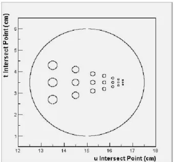
The aluminum phantom, similar to that one used in [7], had50mmexternal diameter and a set of cylindrical holes with diameters ranging from4mmto0.5mm(see Table 1). It was situated att= 35.0mmandu= 150.0mm(central point) like it is shown by Fig.2.
Figure 2. The phantom geometry.
The characteristics of outgoing protons for a given an-gle of the phantom rotation (projection) were determined at thetv-plane, symmetrically situated atu= 30.0mm. The interaction of protons with the air in the phantom holes and on the way to and behind the phantom was neglected. The energy of each outgoing protonEout, and its newt- andv -position were the principal characteristics contained in the program output file. More technical details of the simula-tion can be found in [8].
TABLE 1. The phantom geometry.
Structure D [mm] x0[mm] y0[mm]
hole 1a 4.0 -15.0 8.0
hole 1b 4.0 -15.0 0.0
hole 1c 4.0 -15.0 -8.0
hole 2a 3.0 -5.0 6.0
hole 2b 3.0 -5.0 0.0
hole 2c 3.0 -5.0 -6.0
hole 3a 2.0 2.5 4.0
hole 3b 2.0 2.5 0.0
hole 3c 2.0 2.5 -4.0
hole 4a 1.5 7.5 3.0
hole 4b 1.5 7.5 0.0
hole 4c 1.5 7.5 -3.0
hole 5a 1.0 11.25 2.0
hole 5b 1.0 11.25 0.0
hole 5c 1.0 11.25 -2.0
hole 6a 0.75 13.75 1.5
hole 6b 0.75 13.75 0.0
hole 6c 0.75 13.75 -1.5
hole 7a 0.5 15.625 1.0
hole 7b 0.5 15.625 0.0
hole 7a 0.5 15.625 -1.0
The simulation reported here consisted of a series of180 projections at2-degree intervals with350proton track histo-ries for each projection. In spite of the fact that the180o ro-tation is enough for tomographic image reconstruction, the simulation of the full360orotation of the sample was done to check the reproducibility of the results.
3
Tomographic image reconstruction
To reconstruct the2Dtomographic image of the phantom from the GEANT4simulated data, we used the so-called ”filtered back projection method” [9]. This method is com-monly used in conventionalX-ray CT. In the latter case, the intensity of theX-ray beam that follows a straight pass of lengthLin through a medium is given by:
I(Eγ) =I0(Eγ)·exp
−
L
0
µ(x, Eγ)·dx
(1)
whereµ(x, Eγ)describes the distribution of the linear coefficient of photon absorption along the path. It should be stressed, that the absorption depends not only on the mate-rial of the absorber, but also on theX-ray energyEγ. The energy spectrum of an X-ray tube, I0(Eγ), is an empiri-cally determined complex function of the tube construction and regime of operation.
806 Brazilian Journal of Physics, vol. 34, no. 3A, September, 2004
Sγ(t, ϕ) = ln
N0 N(t, ϕ)
=µmeasured·L (2)
whereN0andN(t, ϕ)are the experimentally registered initialx-ray beam intensity and outgoing beam intensity for the given beam positiontand the angle of CT scanner ro-tationϕ, respectively. (For simplicity, we here assumed the so-called ”1st generation” CT scanner scheme [9].)
In the case of a proton beam, the energy loss can be cal-culated using the expression [4]:
∆E=E0−E=
L
0
µSP(x, Ep)·dx (3)
where we used the non-traditional expression µSP(x, Ep)instead of the commonly useddE/dxfor the local stopping power, just to stress the existing analogy in the equations. The stopping power depends not only on the material, but is also a strong function of the local proton en-ergyEp. The proton energy will significantly change along the path through a thick sample. Thus, when we assume that the initial proton beam energy is maintained along the path, the situation is similar to the case of polychromaticX-rays. The backprojected signal may then be defined as:
Sp(t, ϕ) = ∆E(t, ϕ) =E0−E(t, ϕ) =µSP measured·L
(4) The similarity of expressions (2) and (4) was a strong motivation to use of the same method for the pCT image re-construction as for theX-ray CT reconstruction. Of course, one can expect the same problem - the presence of the so-called ”polychromaticity artifacts” [9] - in the reconstructed images.
4
Results and discussion
As expected, our results were strongly affected by polychro-matic artifacts (see Fig.3 and Fig.4). However, the aim of current investigation was to determine the spatial resolution of the reconstruction method; therefore, we will not further discuss these artifacts, which will have to be resolved if pCT is used for radiotherapy treatment planning [10].
The idea of image reconstruction is based on Nyquist’s theorem, i.e., our signal (projection) should be “sampled” at equal intervals (with a given spatial frequency) [9]. In a real X-ray CT scanner, this is always true, due to its construc-tion (equal translaconstruc-tion moconstruc-tion step for the first generaconstruc-tion CT scanners, or regularX-ray detector cell structure for the last generations).
However, the structure of the simulated proton data is different. The initial t-coordinate of a proton along the width of the parallel beam (see Fig.1) is a random num-ber with uniform distribution between0.0mmand70.0mm. From the experimental point of view, this corresponds to the use of a coordinate sensitive detector with an infinite spa-tial resolution. The same is true for the outgoing protont -coordinate. (For simplicity, we ignored the proton scattering
inv-direction during the current analysis, having in mind the use of a one-sided SSD fort-coordinate determination for the incoming and outgoing protons in a real experiment.)
Figure 3. The result of filtered back projection reconstruction of the proton energy loss data as a function of initial proton position.
Figure 4. The phantom pCT image after data correction assuming straight line approximation.
Thus, before the pCT image reconstruction, the initial and outgoing t-values for each proton in all projections should be rounded to the nearest center of sampling inter-val (hypothetical strip position). A0.2mmstrip pitch was assumed for a virtual (but quite realistic) SSD, and, conse-quently, one can expect a0.4mmlimit of resolution for the reconstructed CT image. A better resolution, although tech-nically possible, is not desirable in our case because under our given conditions (350protons per projection of70.0mm width) this would lead to ”empty rows” in the data matrix.
Ivan Evseevet al. 807
pixel matrix on a0−255gray scale. Using only the
ini-tialt-coordinate versus∆E data leads to the image shown in Fig.3. From the experimental point of view, this corre-sponds to a simple experimental scheme with a single SSD in front of the object, and a proton energy detector with-out position sensitivity behind the object. With this scheme, only the phantom holes of1.5mmdiameter and larger are visible. The presence of strong polychromatic artifacts is also obvious.
An improved pCT image with reasonable contrast and spatial resolution (see Fig.4) was reached when both ini-tial and final coordinates were used to reconstruct a straight-line path of the protons through the phantom. In this case, phantom holes of1mmdiameter can clearly be seen, while the location of smaller holes (0.75mmand0.5mm) can be guessed. The image illustrates the value of correcting the effect of the MCS.
5
Conclusions
A moderate spatial resolution can be achieved by using a position-sensitive proton detector in front of the object, and a proton energy detector without position sensitivity behind the object. If both entrance and exit position are taken into account to determine a straight-path approximation, a much improved resolution can be achieved. Thus, an experimental scheme with two position-sensitive detectors, one situated in the front and the other behind the object, should lead to a reasonably high spatial resolution. Further improvement of the spatial resolution can be expected when using recon-struction techniques that allow incorporation of models of proton MCS better than the straight-line approximation.
Acknowledgments
The authors are very thankful to the Brazilian agencies
CNPq, CAPES and Fundac¸˜ao Arauc´aria for financial sup-port.
R.W.Schulte’s research was sponsored by the U.S. Dept of Army (C/A #DAM D17−97−2−7016) and the
Na-tional Medical Technology Testbed (NMTB), and the con-tent and information does not reflect the position or policy of the U.S. government, or NMTB; no official endorsement should be inferred.
References
[1] E.V. Benton, R.P. Henke, and C.A. Tobias, Science182, 474 (1973).
[2] B.A. de Souza, S.C. Cabral, and R.T. Lopes, Radiation Mea-surements24, 187 (1995).
[3] A.M. Cormack and A.M. Koehler, Phys. Med. Biol.21, 560 (1976).
[4] K.M. Hanson, J.N. Bradbury, T.M. Cannonet.al., Phys. Med. Biol.26, 965 (1981).
[5] K.M. Hanson, J.N. Bradbury, R.A. Koeppe,et.al., Phys. Med. Biol.27, 25 (1982).
[6] GEANT 4 Home Page:
http://wwwinfo.cern.ch/asd/geant4/geant4.html
[7] T. Taylor and L.R. Lupton - Resolution, Artifacts and Design of Computed Tomography Systems - Nuclear Instruments and Methods in Physics Research, A242, 603 (1986). [8] Home Page:
http://scipp.ucsc.edu/ davidw/radiobiology/scan2/.
[9] A.C. Kak and M. Slaney,Principles of Computerized Tomo-graphic Imaging, IEEE Press Inc., N.Y., USA, 1988. [10] U. Schneider, E. Pedroni, and A. Lomax, Phys. Med. Biol.