Quim. Nova, Vol. 30, No. 1, 214-218, 2007
Nota Técnica
*e-mail: [email protected]
PHOTOMULTIPLIER NONLINEAR RESPONSE IN TIME-DOMAIN LASER-INDUCED LUMINESCENCE SPECTROSCOPY
Leandro José Bossy Schip, Bruno Phelippe Buzelatto, Fábio Roberto Batista, Carlos Jorge da Cunha, Lauro Camargo Dias Jr. e João Batista Marques Novo*
Departamento de Química, Universidade Federal do Paraná, CP 19081, 81531-990 Curitiba - PR, Brasil
Recebido em 16/8/05; aceito em 2/3/06; publicado na web em 26/9/06
A new procedure to find the limiting range of the photomultiplier linear response of a low-cost, digital oscilloscope-based time-resolved laser-induced luminescence spectrometer (TRLS), is presented. A systematic investigation on the instrument response function with different signal input terminations, and the relationship between the luminescence intensity reaching the photomultiplier and the measured decay time are described. These investigations establish that setting the maximum intensity of the luminescence signal below 0.3V guarantees, for signal input terminations equal or higher than 99.7 ohm, a linear photomultiplier response. Keywords: photomultiplier; time-resolved; laser-induced luminescence.
INTRODUCTION
Time-Resolved Luminescence Spectroscopy (TRLS) can be implemented by using time- and frequency-domain instrumentations, the simplest ones are built with oscilloscopes, boxcar integrators/ averagers and single-photon detection schemes. Accuracy in excited-state lifetime and time-resolved emission spectra measurements is achieved when the experimental decay curves are obtained under conditions of high signal-to-noise (S/N) ratio, with high time resolution of the instrumentation, by setting a small termination at the oscilloscope or boxcar signal input. For low intensity fluorescent samples it is a common procedure to set the photomultiplier voltage supply close to its typical high voltage value to increase the photomultiplier sensitivity, while keeping the signal input termination at the oscilloscope or boxcar to 50 Ω, to get the highest time-resolution on the instrument. However, by doing so, a distortion of the luminescence signal was obtained in our instrumentation. Photomultiplier tubes provide good linearity in anode output current over a wide range of incident light levels; in other words, they offer a wide dynamic range. However, if the incident light is too intense, the output begins to deviate from the ideal linearity. This is primarily caused by anode linearity characteristics, that are dependent only on the current value if the supply voltage is constant, being independent of the incident light wavelength. This kind of detector nonlinearity has been previously reported in a number of instruments1-8, but here, we present a new procedure to achieve the
photomultiplier linearity range, consisting of extraction of time-resolved laser intensity profile and instrument response function, to be further used in reconvolution methods9 -12 for excited-state lifetime
measurements. We report in this paper a systematic investigation on the supply voltage applied to the photomultiplier; the instrument response function with different signal input terminations; the relationship between the luminescence intensity reaching the photomultiplier and the measured decay time; and the extraction of the laser intensity profile in time-resolved luminescence measurements.
EXPERIMENTAL The instrumentation
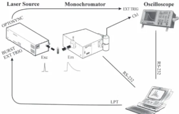
The instrumentation (Figure 1) is set up with a Thermo Laser Science mod. VSL-337ND-S (Oriel mod. 79070) pulsed nitrogen laser13 (λ
em = 337,1 nm; < 4 ns Full-Width at Half-Maximum,
FWHM) for the photo-excitation of the sample; a 1/4 m Oriel Cornerstone 260 emission monochromator14 for the spectral
resolution of the luminescence emission, coupled to an Oriel diffraction grating mod. 74063 (0.15 nm resolution at 546.1 nm, 1200 lines/mm, blaze at 350 nm), an Oriel mod. 59470 (Schott GG385) color glass filter to block the excitation light at the micrometer-driven entrance slit, and an Oriel mod. 77348 fast (2,2 ns rise-time) side-on photomultiplier tube at the micrometer-driven exit slit; a Tektronix mod. TDS3032B (300 MHz, 2 channels, 2,5 GSamples/s) Digital Oscilloscope15 to detect the signal. To be
appropriated to TRLS, the oscilloscope must meet requirements on
time resolution (1.2 ns rise-time and 0.4 ns sampling time for the mentioned oscilloscope), pre-trigger signal acquisition ability (signal waveform capture before the trigger is detected by the oscilloscope), the averaging mode acquisition (for improvement of the signal-to-noise ratio) and digital precision for the waveform acquisition (9-bits for the “sample” acquisition mode and 14-bits for the “average” mode). To acquire low intensity luminescence emission at the nanosecond time scale, an additional pre-amplifier could be used for signal amplification, but that was not used in this work. The PC-compatible computer must have at least two serial communication ports (named RS-232 in the figure) and one parallel port16 (named LPT) to control the oscilloscope, the monochromator
and the laser, respectively. Both the oscilloscope and the monochromator have a built-in GPIB (IEEE-488) interface, but the lower cost serial ports (RS-232 standard interface) were preferred in this work. The source code was developed in BASIC.
The laser used in this work is a new model that has several input and output connections that enable it to be computer controlled. Two input ports, BURST and EXT_TRIG, are used to control the electrical charging and the firing of the laser plasma tube, respectively. These controls save the plasma tube lifetime because the laser is fired only when the oscilloscope is ready for the signal acquisition. A third port, OPTOSYNC, is used to synchronize the laser firing with the signal acquisition by the oscilloscope, with low (less than 1ns standard deviation) time jitter.
The software automatically adjusts some oscilloscope parameters for TRLS data acquisition, such as: vertical menu, for channel 1 (input signal from photomultiplier): Coupling = DC; internal termination = 1 MΩ (Observation: the external termination is chosen by the user and must be appropriated for the time resolution of the experiment); Invert = On; Bandwidth= Full; trigger menu (input trigger from OPTOSYNC laser pulse): Type = Edge; Source = EXT/ 10; Coupling = DC; Slope = Rising edge; Level = 1.3 V; Mode = Normal.
Finally, a home-made metallic sample holder was built to accept either a standard 10 mm-optical path length fluorescence quartz cuvette for liquids or 0.01 mm-optical path length quartz windows for powdered samples.
Decay analysis
The decay curves in this work were analyzed with the recommended method17 of Levenberg-Marquardt least-squares18,
using 500 points per each curve. Deconvolutions18 were performed
with a spreadsheet.
THEORETICAL BACKGROUND
Response time of the instrument and signal input termination The knowledge of the instrument response time (or RC time constant of the electric circuitry), is very important because it may distort and limit the time resolution of the experimental data. As an example, the time-dependent photon flux signal reaching the photomultiplier is converted to electrical current, and its temporal profile can be seriously distorted by sources of resistance and capacitance of the instrument12 like termination (resistance R
term) at
the oscilloscope signal input, internal resistance and capacitance from the oscilloscope (Rosc, Cosc), photomultiplier (RPMT, CPMT) and the cable connecting the photomultiplier to the oscilloscope (Ccable). All these resistances and capacitances are connected in parallel and thus the reciprocal of the RC response time of the instrument, Equation 1, can be easily derived through the following steps:
R-1 = R PMT
-1 + R osc
-1 + R term
-1
C = CPMT + Ccable + Cosc (RC)-1 = (R
PMT -1 + R
osc -1 + R
term -1) × C-1
(RC)-1 = (R PMT
-1 + R osc
-1) × C-1 + C-1× R term
-1
(RC)-1 = Constant + C-1× R term
-1 (1)
Equation 1 shows that a linear relationship between (RC)-1 and
Rterm-1 should be expected when the external termination at the
oscilloscope signal input is changed.
Instrument response function and time-resolved laser intensity profile:
The true time-dependent decay of a luminescent sample (also known as Impulse Response Function, IRF) can be recorded when the sample is illuminated by a δ-function excitation pulse, and its emission is detected by an ideal equipment, possessing a δ-function instrument response, SR. However, real excitation sources and detection equipments show finite temporal-profile, I0(t), and finite instrument time-response, SR(t), respectively. Therefore, the recorded fluorescence decay, F(t), can be described by the convolution of the IRF(t), SR(t), and I0(t) functions (Equation 2).
F(t) = IRF(t) ⊗ SR(t) ⊗ I0(t) (2)
The sample’s true luminescence decay, IRF, can be therefore extracted by least-squares reconvolution methods, using SR and I0 functions.
RESULTS AND DISCUSSION
In this work, we acquired time-resolved spectra and decay cur-ves of the nitrogen laser and of the uranyl nitrate hexahydrate emissions, with different terminations. The temporal and spectral profiles of the nitrogen laser emission, and of the uranyl nitrate hexahydrate emission (Figure 2) exemplify the TRLS data that can be obtained with this instrumentation. The systematic investigations that were conducted are discussed in detail below.
Supply voltage applied to the photomultiplier and noise sources
Attempts to set the photomultiplier supply voltage to its typical value (-1000V) produced nonlinear distortion in the measurements and at least three sources of noise are present in this instrumentation: Johnson noise (thermal noise), caused by the random motion of carriers in a conductor and resulting in fluctuations in the internal resistance of the detector. The amplitude of this random noise was observed to be within the range –0.46 mV to +0.46 mV (This noise amplitude is within the 1 mV/div minimum vertical scale of the oscilloscope). Shot noise, composed of photons arriving the photomultiplier randomly in time. The manufacturer recommends19
to make this noise three times bigger than the Johnson noise, in order to measure signals with a high degree of linearity. The observed shot noise amplitude was within the range 0 to +1.4 mV, with -600V applied to the photomultiplier tube. Electromagnetic interference (EMI) of the laser plasma tube discharge, that appears in all signal and baseline acquisitions as a pattern within the range of –2.25 mV to +2.25 mV when the laser is fired. The acquisition software disables the laser plasma tube charging during the data acquisition, to avoid extra EMI noise.
be minimized by subtracting a baseline signal, previously acquired with the monochromator shutter closed. With this procedure, a 4 mV ampli-tude laser EMI noise in the original signal was reduced to 1 mV, matching the amplitude of the Johnson noise. All decay curves reported in this paper were previously submitted to such baseline subtraction.
Instrument Response Function with different signal input terminations
From Equation 1 a linear relationship between (RC)-1 and R term
-1
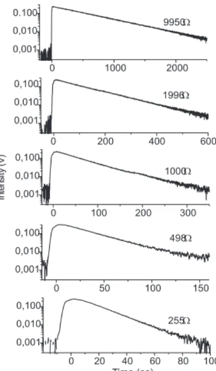
should be expected when the external termination at the oscilloscope signal input is changed. To verify this, a series of decay curves were acquired by setting the monochromator to the laser emission (λ = 336.93 nm), with seven different terminations at the oscilloscope signal input. Five acquired curves are shown as semilogarithmic plots in Figure 3. The four upper curves (9950 Ω, 1996 Ω, 1000 Ω and 498 Ω) in this figure have an acceptable linearity because the laser pulse duration was shorter than the decay time scale and, therefore, they follow the exponential decay defined by the RC time constant of the instrumentation. The curves acquired with terminations 255 Ω and 99.7 Ω (not shown in Figure 3) were acquired with the photomultiplier within its linear response range, but the decay deviate considerably from the linearity because the laser width is comparable to the decay time scale. The least-squares fit, within the linear region of the four upper curves, assuming V = Vmax × exp(-t/RC), gave the parameter RC for each termination. The relationship between RC-1 and R
term -1 has a
linear correlation coefficient of 0.99998, which is in agreement with Equation 1, and that was used to extrapolate the RC response time of
the instrument for the three lower terminations (Table 1). Note that for these fast signals (laser emission), the maximum anode current with termination 99.7 Ω is 20 times higher than that with termination 1996 Ω (Table 1). In the last section we will see evidences that with terminations 255 and 99.7 Ω the photomultiplier still operates in its linear region.
Relationship between the luminescence intensity reaching the photomultiplier and the measured decay time
The investigation of the photomultiplier behavior was performed in two independent experiments: (1) acquisition of a faster signal (laser emission, < 4ns Full-Width-at-Half-Maximum, FWHM), and (2) acquisition of a slower signal (685 µs luminescence decay of Table 1. Response time of the instrument, RC, for different termi-nations (Rterm) used in this work, calculated with equation (RC)-1 = Constant + C-1× R
term
-1, where Constant = (-5.135 ± 8) 104 s-1 and
C-1 = (1601 ± 7)107 F-1. The last column gives the estimated
photo-multiplier anode current (ianode, max = Vmax/Rterm), assuming Vmax = 0.3 V for all decay curves observed at the oscilloscope screen
Termination, Response time of Estimated anode
Rterm (Ω) the instrument, current,
RC (ns) ianode, max (µA)
49.8 3.1111 6024
99.7 6.2301 3009
255 15.941 1176
498 31.16 602
1000 62.66 300
1996 125.5 150
9950 642.0 30
1 Extrapolated values
Figure 2. Examples of two-dimensional data obtained with the instrumentation: Time-Resolved Luminescence Spectra and luminescence decays of the laser emission (top), acquired with 99.7 Ω termination at the oscilloscope signal input, and uranyl nitrate hexahydrate emission (bottom). Each decay curves were obtained with 10000 points, but only 100 points for each decay are displayed in the figure for clarity
uranyl nitrate hexahydrate) than the 125.5 ns response time of the instrumentation, with the 1996 Ω termination at the oscillos-cope signal input.
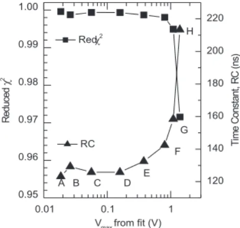
Experiment 1: The photomultiplier linearity range was investigated by acquiring decay curves of the laser emission (λ = 336.97 nm), at different slit widths in the monochromator. In this experiment, the laser can be considered as a delta function and the observed curves follow the exponential RC decay of the electrical circuitry of the instrumentation. The least-squares fit of these curves, between 50 and 500 ns, assuming V = Vmax × exp(-t/RC), gave the parameters Vmax (maximum intensity at zero time, in volts), RC, and the reduced least-squares sum (Reduced χ2) that are plotted in
Figu-re 4. This FiguFigu-re shows that RC is nearly constant at 126 ns and the Reduced χ2 is greater than 0.998 when V
max is below 0.3 V. Therefore,
this 0.3 V value corresponds to the maximum signal voltage that assures the acceptable linear response for the photomultiplier. Thus, the maximum anode current at the photomultiplier, under these conditions, is 150 µA, higher than that reported by manufacturer’s specifications (100 µA, for a DC signal).
Experiment 2: The linearity range was investigated by acquiring decay curves of the luminescence emission of solid uranyl nitrate hexahydrate (λmax = 510 nm), using different slit widths at the monochromator. In this experiment, the observed decay curve follows the characteristic excited-state decay of the uranyl nitrate. The
least-squares fit of these curves, between 0.7 and 2.5 ms, assuming V = Vmax × exp(-t/τ), gave the fitted parameters Vmax, τ, and Reduced χ2, that are plotted in Figure 5. This Figure shows that τ is
nearly constant at 685 µs and the reduced χ2 is greater than 0.97
when Vmax reaching the photomultiplier is below 1.0V for 1996 Ω termination. Therefore, this 1.0V value corresponds to the maximum signal voltage that assures the acceptable linear response for the photomultiplier for slow signals. Thus, the maximum anode current at the photomultiplier, under these conditions, is 501 µA, higher than that reported by manufacturer’s specifications. The 685 µs value obtained for the lifetime of solid uranyl nitrate hexahydrate is in very good agreement with the values 695 µs20 and 719 µs21 found in
the literature, showing the accuracy of the instrumentation. In these two experiments, the lowest limit for the photomultiplier response range is given by both, the 5mV/div vertical scale limit (for full 300MHz bandwidth) at the oscilloscope and by the noise magnitude. These two experiments show that the maximum intensity limit to achieve linearity in the photomultiplier response can be extended over its reported maximum DC anode current.
Extraction of the time-resolved laser intensity profile
The extraction of the time-resolved laser intensity profile was done with the TRLS surfaces of the laser pulse with 99.7 Ω (Figu-re 2), 255 Ω and 498 Ω terminations. Figure 6 shows that the FWHM of the baseline-corrected signals, acquired at 336.93 nm, are 14.4, 21.8 and 34.4 ns for the three terminations, respectively. The curves observed at the oscilloscope are distorted by the RC response time of the instrument and they are the result of the convolution of the real laser pulse temporal profile with the RC response of the instrument. Therefore, in order to extract the “true” laser pulse profile from these observed curves, a deconvolution between the observed (distorted) signal and the RC decay function of the instrument must be performed. The RC decay functions were assumed to be a single exponential decay with RC equal to 6.230, 15.94 and 31.16 ns, for that three terminations, respectively (Table 1 – Observation: the 6.230 and 15.94 ns RC time constants were obtained by extrapolation of Equation 1). The deconvoluted curves showed a FWHM laser profile with 3.4, 3.0 and 3.2 ns, for the 99.7, 255 and 498 Ω terminations, respectively, which are in excellent agreement with the manufacturer’s specification (< 4 ns FWHM). These consistent results show that the Figure 4. Instrument decay time constant (RC) and reduced least-squares
sum (Reduced χ2) versus maximum intensity (V
max) obtained by the least-squares fit of the laser emission decay curves
Figure 5. Decay time and reduced least-squares sum (Reduced χ2) versus maximum intensity (Vmax) obtained by the least-squares fit of the uranyl nitrate hexahydrate emission decay curves
photomultiplier still operates within its linear response range, for the terminations 99.7, 255 and 498 Ω. The laser widths obtained fluctuate within 0.4 ns, as we are working at the time limit of the instrumentation, this fluctuation can be assign to the maximum sampling rate of the oscilloscope and to the temporal jitter of the OPTOSYNC trigger pulse. The deconvolution of the signal acquired with the 49.8 Ω termination and with 0.13V maximum intensity, gave a 4.8 ns FWHM laser profile showing that for these settings the photomultiplier response is no longer linear.
CONCLUSION
The goal of the present work was the investigation of the photomultiplier nonlinear response when it is illuminated with pulsed light, in time-domain luminescence experiments. To achieve the photomultiplier linear response range, several investigations had to be performed, such as: (i) Effect of the supply voltage applied to the photomultiplier; (ii) Instrument Response Function with different signal input terminations; (iii) Relationship between the luminescence intensity reaching the photomultiplier and the measured decay time; and (iv) Extraction of the time-resolved laser intensity profile. These investigations showed that the photo-multiplier linear response can be achieved by a simple visual inspection at the oscilloscope screen: Setting the maximum intensity of the luminescence signal below 0.3V guarantees that, for signal input terminations equal or higher than 99.7 ohm, the photomultiplier response is linear. For signals with intensities higher than 0.3V, the photomultiplier response is nonlinear and a distorted decay curve is observed at the oscilloscope. The lowest limit for the photomultiplier linear response is given by the shot noise amplitude, 1.4mV, achieved by setting the photomultiplier high voltage supply to –600V, with the laser EMI noise amplitude minimized by baseline subtraction. The instrumentation presented in this paper is being used for the characterization of photophysical and photochemical processes in intercalation compounds, macrocyclic complexes, conducting polymers, and photochromic materials by least-squares Levenberg-Marquardt global analysis, whose source code was recently developed in our laboratories. Further improvement in this source code will be made, by the use of the time-resolved laser intensity profile and the instrument response function with reconvolution methods, for the extraction of the excited-state lifetime of luminescence samples at the nanosecond time scale.
ACKNOWLEDGMENTS
To Prof. Dr. F. B. T. Pessine (Institute of Chemistry, IQ-UNICAMP), Prof. Dr. F. Y. Fujiwara (IQ-IQ-UNICAMP), Prof. Dr. I. Mazzaro (Department of Physics, UFPR), and Mr. E. Bento. J. B. M. Novo is indebted to Fundação Araucária / SETI / PR for financial support for this research.
REFERENCES
1. Fang, Q.; Papaioannou, T.; Jo, J. A.; Vaitha, R.; Shastry, K.; Marcu, L.; Rev.
Sci. Instrum.2004, 75, 151.
2. Yotter, R. A.; Wilson, D. M.; IEEE Sensors J.2003, 3, 288. 3. Iwata, T.; Takasu, T.; Araki, T.; Appl. Spectrosc.2003, 57, 1145. 4. Vicic, M.; Sobotka, L. G.; Williamson, J. F.; Charity, R. J.; Elson, J. M.;
Nuclear Instrum. Methods Phys. Res., Sect. A 2003, 507, 636.
5. Xiao, M.; Selvin, P. R.; Rev. Sci. Instrum.1999, 70, 3877. 6. Alfano, A. J.; Appl. Spectrosc.1998, 52, 303.
7. Vasilchenko, Y. V.; Zhavoronkov, N. A.; Padalko, V. N.; Instruments and
Experimental Techniques1996, 39, 552.
8. Wirth, M. J.; Burbage, J. D.; Zulli, S. L.; Applied Optics1993, 32, 976. 9. Vecer, J.; Kowalczyk, A. A.; Dale, R. E.; Rev. Sci. Instrum. 1993, 64, 3403. 10. Vecer, J.; Kowalczyk, A. A.; Davenport, L.; Dale, R. E.; Rev. Sci. Instrum.
1993, 64, 3413.
11. Wahl, Ph.; Auchet, J. C.; Donzel, B.; Rev. Sci. Instrum.1974, 45, 28. 12. Demas, J. N., Excited State Lifetime Measurements, Academic Press: New
York, 1983.
13. Thermo Laser Science; VSL-337 ND-S Nitrogen Laser 337201-00/01 User
Manual, Laser Science Inc.: Franklin, 1995.
14. Thermo Oriel; Cornerstone 260 1/4m Monocromator Instruction Manual,
Thermo Oriel: Stratford, 2001.
15. Tektronix; Programmer Manual - TDS3000 & TDS3000B Series Digital
Phosphor Oscilloscopes 071-0381-02, Tektronix Inc.: Beaverton, 2002.
16. VanBommel, G.; Quinn, W. R.; Rev. Sci. Instrum.1987, 58, 2346. A short description of an optocoupler isolation circuit and BASIC commands to access the parallel printer interface are described. We plugged the parallel pins of the computer directly to the laser external trigger and burst inputs because this laser model from Laser Science is already protected with internal opto-isolators for minimizing EMI/RF interferences.
17. Eaton, D. F.; Pure Appl. Chem.1990, 62, 1631
18. Press, W. H.; Teukolski, S. A.; Vettereing, W. T.; Flannery, B. P.; Numerical
Recipes in Fortran 77: The art of scientific computing, 2nd ed, Cambridge
University Press: Cambridge, 1986, chap. 13.1 and 15.5.
19. Oriel Instruments; The Book of Photon Tools, Oriel Instruments: Stratford, USA.