ISSN 0100-2945 http://dx.doi.org/10.1590/0100-29452016533
PLOT SIZE IN THE EVALUATION OF PAPAYA SEEDLINGS
‘BAIXINHO DE SANTA AMÁLIA’ IN TUBES
1HUMBERTO FELIPE CELANTI2, OMAR SCHMILDT3, RODRIGO SOBREIRA ALEXANDRE4,
LAERCIO FRANCISCO CATTANEO5, EDILSON ROMAIS SCHMILDT6
ABSTRACT- Were evaluated three characters in papaya seedlings ‘Baixinho de Santa Amália’ to estimate the optimum plot size and the number of replications in a completely randomized experiment, a randomized block and Latin square. The characters were seedling height, leaf number and length of roots from uniformity test with 240 seedlings. The determination of the optimum plot size was done by applying the method of Hatheway (1961). The number of seedlings per plot for seedling production is variable depending on the number of treatments and replications assumed precision, the character in question and the experimental design. Comparing designs, the plot size is greater in the Latin square, followed by a randomized block design and completely randomized, and this difference is more pronounced the lower the number of treatments
and replicates used. For the same number of treatments and the same precision, the most efficient use of the
experimental area is given using smaller plot, with more replications, which require less space in the nursery than larger plots with fewer replications. For experiments completely randomized and randomized blocks
with five or more treatments, four replications, and precision of 15% around the mean, it is recommended
to use nine seedlings per plot.
Index terms: Carica papaya L.,experimental precision, experimental planning, design experimental.
TAMANHO DE PARCELA NA AVALIAÇÃO DE MUDAS DE MAMOEIRO
‘BAIXINHO DE SANTA AMÁLIA’ EM TUBETES
RESUMO- Foram avaliados três caracteres em plântulas de mamoeiro ‘Baixinho de Santa Amália’ com objetivo de estimar o tamanho ótimo de parcelas e o número de repetições em experimento inteiramente ao acaso, em blocos ao acaso e em quadrado latino. Os caracteres foram altura da plântula, número de folhas e comprimento da maior raiz a partir de ensaio em branco com 240 plântulas. A determinação do tamanho ótimo de parcela foi feita aplicando-se o método de Hatheway (1961). O número de plântulas por parcela para produção de mudas é variável em função do número de tratamentos e de repetições, precisão assumida, do caráter em questão e do delineamento experimental. Na comparação entre delineamentos, o tamanho de parcela é maior no quadrado latino, seguido de blocos ao acaso e inteiramente ao acaso, sendo que esta diferença é mais acentuada quanto menor for o número de tratamentos e de repetições. Para um mesmo número
de tratamentos e mesma precisão, o uso mais eficiente de área experimental se dá utilizando-se parcelas
menores, com maior número de repetições, as quais demandam menor espaço em viveiro do que parcelas maiores, com menor número de repetições. Para experimentos inteiramente ao acaso e em blocos ao acaso
com cinco ou mais tratamentos, quatro repetições, e, precisão de 15% em torno da média, recomenda-se o
uso de nove plântulas por parcela.
Termos para indexação: Carica papaya L., precisão experimental, planejamento experimental, delineamentos experimentais.
1(Trabalho 093-15). Recebido em: 13-04-2015. Aceito para publicação em: 11-06-2016.
2Eng. Agr., Ms., Laboratório de Melhoramento de Plantas, Universidade Federal do Espírito Santo, CEUNES, São Mateus, ES. E.mail: [email protected]
3Eng. Agr., Dr., Pós Doutorando (PNPD/CAPES), Deptº de Ciências Agrárias e Biológicas, Universidade Federal do Espírito Santo, CEUNES, São Mateus, ES. E-mail: [email protected]
4Eng. Agr., Dr., Professor, Deptº de Ciências Florestais e da Madeira, Universidade Federal do Espírito Santo, CCAUFES, Jerônimo Monteiro, ES. E-mail: [email protected]
INTRODUCTION
In conducting any experiment must begin with proper planning. In this planning, after having been determined the characters to be studied, and what design will be adopted, the researcher begins to quantify how much material will be required to perform the test, and this should determine the size of each plot (FIRMINO et al., 2012). Although the majority of researchers still choose to determine the size of the plot of arbitrary shape, the ideal is to
make that choice based on scientific criteria, which
typically involve the use of uniformity tests, also called blank test. In these tests, is demonstrated that there is nonlinear relationship between the experimental error and the size of the plot (SMITH, 1938; MEIER; LESSMAN, 1971). Although the researcher wants to reduce experimental error (STORCK et al., 2011; BRITO et al., 2012), and to this increases the plot size, this criterion should be done with caution, since, from a certain increase of the plot size, reducing experimental error is greatly reduced (PIMENTEL-GOMES, 2009), leading to spending experimental material and unnecessary physical space. Thus, seek to the optimum plot size (MEIER; LESSMAN, 1971; PARANAÍBA et al., 2009; LORENTZ et al., 2012).
About the method for determining the optimal size of the plot, the literature reports more than a dozen proposals, and most often used is the
maximum modified curvature (MEIER; LESSMAN,
1971). Recently, some works are carried out with new methodological approaches to this question, giving methods such as maximum curvature of
the coefficient of variation and the linear response
with plateau (PARANAÍBA et al., 2009), the anti-tonic regression method (BRITO et al., 2012), the maximum distance method (LORENTZ et al., 2012), and method involving the bootstrap simulation with replacement (BRITO et al., 2014). All these methods allow us only the determining portion size, without resource to determine the number of the involved plots, which can be obtained, however, by the method
of Hatheway (1961). By this method can be satisfied
the longings of the researcher who wants to know the optimum plot size for your research reality, which also includes the number of treatments and replications, the experimental design used and the precision of the experiment.
Studies by determination of the plot size
can be made for various environment as the field
(CARGNELUTTI FILHO et al., 2014; LEONARDO et al., 2014), laboratory (PEIXOTO et al., 2011; MORAIS et al., 2014) and in the nursery (CIPRIANO
et al., 2012; FIRMINO et al., 2012). In studies with production of papaya, in tubes, in nursery, useful portion sizes follow an arbitrary, given the inexistence of plot dimensioning studies. Are reported the evaluation of experiments with four plot sizes (MELO et al., 2007), six (SÁ et al., 2013), nine (OLIVEIRA FILHO et al., 2013), ten (PAIXÃO et al., 2012; MENGARDA et al., 2014) and twelve (SERRANO et al., 2010) useful papaya seedlings per plot.
This study aimed to determine the optimal size of plots in the evaluation of papaya seedlings ‘Baixinho de Santa Amália’, in tubes, for experimental design completely randomized, in a randomized blocks and Latin square, using the method of Hatheway (1961).
MATERIALS END METHODS
The study was conducted in October 2013, in a greenhouse at the Experimental Farm of CEUNES/ UFES, in São Mateus, northern city in the state of Espirito Santo, typical papaya producer in Brazil, which is located between 18°40’19.6” south latitude and 39°51’23.7” west longitude. The climate is the AWI type (humid tropical), with rains in summer and dry winter. The greenhouse used has coverage arc, benching with height of 0.5 m for placement of trays, the side and front walls are anti-aphid screen, the roof
covered with polyethylene film of 150 microns, the floor covered with crushed rock and micro sprinkler
irrigation automatic.
Determining the optimal size of plots
was made with papaya seedlings (Carica papaya
L.) cv. Baixinho de Santa Amália, whose seeds were obtained from the germplasm bank of the Caliman Agrícola Company S/A. The blank test was conducted using three black polyethylene trays containing 10x14 tubetes de 50 cm3. The trays were allocated on the stands together to provide 14 rows of 30 tubes, a total of 420 tubes. In October 2013, were seeded all 420 tubes being utilized to evaluate only the seedlings of the eight central rows, which corresponds to 240 seedlings, as shown in Figure 1.
the “tipping” or “damping-off” (Rhizoctonia solani
Khun) given that were not carried out phytosanitary treatments.
The characteristics evaluated at 30 days after sowing were: SH: seedling height, determined with ruler graduated in centimeters, measuring from the base of the stem to the apex of the last leaf; NL: number of leaves, by counting the developed true leaves; and, LRL: the longest root length, determined by measuring from the base of the seedling to end thereof with ruler graduated in centimeters.
To determine the optimum plot size (X0) it was used the second method of Hatheway (1961). By this method, from the blank test is possible to determine for the X0 to different experimental accuracies, as demonstrated by Henriques Neto et al. (2004) and Cargnelutti Filho et al. (2014).
Thus, was structured 240 seedlings of the blank test in basic experimental units (BEU), from the eight rows of 30 seedling trays (Figure 1), where each BEU foi was constituted by one seedling. The BEU were added, using a number of exact divisors of the total number of seedlings in the seedling of the blank test varying from 1 to 60 BEU, constituting
13 groupings. For each specific grouping, it was
observed all the possibilities of grouping composition for evaluating seedling characters within each of the eight rows (WR) 30 seedlings or seedlings between the rows (BR). Thus, the sizes of the groupings (Xi) were in BEU: X1 = 1 (1WR x 1BR); X2 = 2 (1WR x 2 BR, 2WR x 1 BR); X3 = 3 (3WR x 1 BR); X4 = 4 (1WR x 4 BR e 2WR x 2 BR); X5 = 5 (5WR x 1 BR); X6 = 6 (6WR x 1 BR e 3WR x 2 BR); X8 = 8 (1WR
x 8 BR e 2WR x 4 BR); X10 = 10 (10WR x 1 BR e
5WR x 2 BR); X12 = 12 (6WR x 2 BR e 3WR x 4
BR); X15 = 15 (15WR x 1 BR); X20 = 20 (10WR x 2 BR e 5WR x 4 BR); X30 = 30 (30WR x 1 BR e 15WR x 2 BR); X60 = 60 (30WR x 2 BR e 15WR x 4 BR).
The evaluation of height, number of leaves and the longest root length of seedlings, for each of Xi BEU is calculated: m(Xi) , mean plots with Xi BEU of size;V(Xi), variance between plots with Xi BEU of size; CV(Xi), coefficient of variation between plots with Xi BEU of size; and VU(Xi) = V (Xi)/ X2
i, variance by BEU between plots of Xi BEU of size. From the relation of
VU(Xi) in function of Xi, it was determined heterogeneity index (b) from of the logarithmic function in base 10 of the equationVU(Xi)= V1/Xb
1, according to Smith (1938), with weighting by the degrees of freedom associated with the number of applicable plots of size Xi BEU for each plot size planned in the blank test (STEEL et al., 1997).
For each character evaluated were simulated experimental designs for the designs completely
randomized (DCR), in randomized blocks (DRB) and Latin square (DLS), for the scenarios formed by combinations of I treatments (I = 3, 4, ..., 30), r replications (r = 2, 3, ..., 10) end d differences
between treatment mean being detected as significant at the 5% probability, express in percent of overall mean of the blank test (d = 5, 10, 15 e 20%).
As reported by Cargnelutti Filho et al. (2014), the d indicates precision, being that, small percentage of d indicates greater precision, in other words the small differences between treatment mean
will be considered significant. In the simulations, the
criteria for combinations take into consideration: the lowest number of treatments was three (I = 3), whereas that the detection of the difference between two mean can now be made by analysis of variance; the smallest number of replications was 2 (r = 2), because this is the minimum for detecting the experimental error; the I treatments and r replications were combined to provide a minimum of 20 plots per experiment, according to Pimentel Gomes (2009) recommendation; to DLS were simulated only combinations that provide size of 25 (I = 5; r = 5), 36 (I = 6; r = 6), 49 (I = 7; r = 7), 64 (I = 8; r = 8), 81 (I = 9; r = 9) and, 100 (I = 10; r = 10) plots, as this is a requirement for analysis by DLS, on which I2 = n plots; for I greater than 10, was only evaluated combinations of I = 15, I = 20, I = 25 and, I =30 with r = 2, r = 3, r = 4 and r = 5 for a DCR and DRB.
In each character (HS, NL e LRL), for each experimental design and the outlining DCR, DRB and DLS, was calculated the optimum plot size (X0), in number of BEU, by means of the method of Hatheway (1961), given by .
In this equation, it follows that: b is the heterogeneity index Smith Smith (1938); CV is the
estimate of the coefficient of variation between plots
of one BEU of size, in percentage; r is the number of replications considered; d is the difference between
treatment mean to be detected as significant at the 5%
probability, expressed as a percentage of the overall mean of the blank test; t1 is the tabulated value of
t for significance tests (5% two-sided test) with df
degrees of freedom; t2 is the tabulated value of t bilateral, corresponding to an error of 2 (1-p) with degrees of freedom df, with p = 0.80 the probability
of significant results.
The tabulated values of t distribution were obtained with residue degrees of freedom df, according to the treatments I and r replications, where gl = I(r – 1) for a DIC, df = (I - 1)(r – 1) for a DRB and, df = (I - 1)(I – 2) for a DLS.
The basic experimental units (BEU) of the same size Xi BEU and different shapes have been
grouped to form 13 sizes of Xi UEB upon which the analysis was carried out.
The data have been analyzed using the computational resources of the R software (R Development Core Team, 2014). Since this is a discrete random variable, the optimum plot size was presented by integer number, adopting rounding to whole number.
RESULTS AND DISCUSSION
In 10 days after sowing (DAS),
95.83% of the seeds were emerged.
And then was made the substitution of 10 tubes who did not have emerged seeds, so that in 30 DAS could be evaluated 240 seedlings of the blank test.
There was mean increase in plots [m(Xi)]
and, decrease the coefficient of variation [CV(Xi)] and variance by BEU between plots [VU(xi)],with increasing planned plot size, measured in number of BEU (Table 1). The mean seedling height (SH), number of leaves (NF) and the longest root length (LNR), was of 6.47cm; 3.49 leaves e 13.50cm, respectively, this shows that the seedlings were in acclimation conditions for further planting in the field. This statement can be made especially in relation to LRL since seedlings with very small roots tend to suffer more in the initial stage of growth in
the field. In the production of papaya, Serrano et al. (2010) in the evaluation of five cultivars, Paixão et
al. (2012) in the evaluation of ‘Golden THB’ and, Mengarda et al. (2014) in the evaluation of four cultivars, obtained similar results in root length, in the evaluation at 30, 30 and 45 DAS, respectively.
The coefficient of variation between 240 BEU
was different between the SH characters, NL and
LRL, with values of 14.03%; 20.29% and 17.78%, respectively. Different coefficients of variation for
different characters in the same plants were also detected in the production of Catuaí Yellow 2SL coffee seedlings (FIRMINO et al., 2012) and Rubi coffee (CIPRIANO et al., 2012). Presence of variability
between the BEU, measured by the coefficient of
variation (CV) and the heterogeneity index (b), are important for the study of the optimum plot size by method of Hatheway (1961). In this research, the values of b were 0.667 para AP, 0.967 for a NL and 0.973 for a LRL (Figure 2). Thus, it is observed by the expression X0 = √2(t1+t2)2 CV2/rd2 that for the same number r of replications, I of treatment, the same d precision and the same experimental design, there is greater plot size trend (X0) for characters with higher CV, and the opposite occurs with respect to
b. Thus, as the CV values and b are uncorrelated, Xo also it depends on which precision (d) was assumed.
It was considered a DCR, DRB and DLS with five treatments and five replications, the larger portion
size will be for AP when considering d = 5 and d =
10% around the mean, and to NL when considering d = 15% or more (Table 2, 3, 4).
Over the years, many papaya farmers have improved the seedling production system. The seedlings that were prepared in polyethylene bags with about 500 cm3 of substrate, with soil, could be substituted for plastic tubes with volume of commercial substrate only 50 cm3. Thus, it decreases the probability of spread of disease by the substrate and also the space spent in the nursery, the same amount of production seedlings. In the case of research involving the production of seedlings in plastic tubes, one of the researcher’s wishes is also to decrease the space spent in the nursery. This can be achieved, according to the equation presented by Hatheway (1961); by the assumed precision (d), by the arrangement between the number of replications (r), and also due to the assumed experimental design. These options can be assumed individually or together.
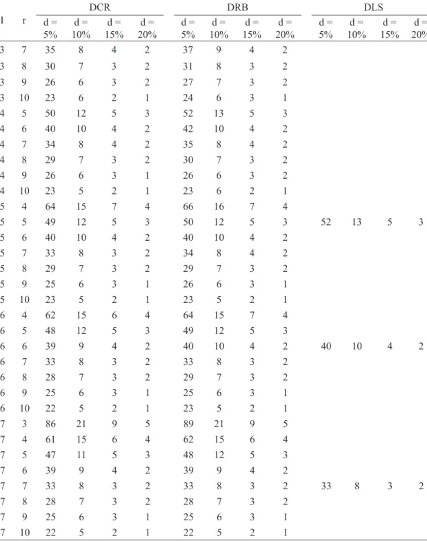
In the case of working with d, it is observed that X0 is greater how bigger the d, considering the same character, the same number of treatments and replications, as can be observed to SH (Table 2), NL (Table 3) and LRL (Table 4).
The researcher, however, should do so with caution. Taking as an example the character SH, is
assumed precision of 20% (d = 20%), in a DRB,
with 5 treatments and 4 replications, X0 = 2BEU. However, when analyzing, in Figure 2a, the plot size as 3 BEU corresponds to high variance per basic experimental unit (BEU) between the plots of Xi UEB of size [VU(Xi)]. In this example, it is more
prudent to use d = 15%, which corresponds to X0 = 7 BEU, which as can be seen, It shows small change in VU(Xi) from this plot size (Table 2). However, larger size is required when considering NL that requires X0 = 9 seedlings per plot, which approximates to the useful plot size assumed by other researchers in research with seedlings in tubes of other varieties of papaya (SERRANO et al., 2010; PAIXÃO et al., 2012; OLIVEIRA FILHO et al., 2013; SÁ et al., 2013; MENGARDA et al., 2014).
In case it is desired to more efficient use of
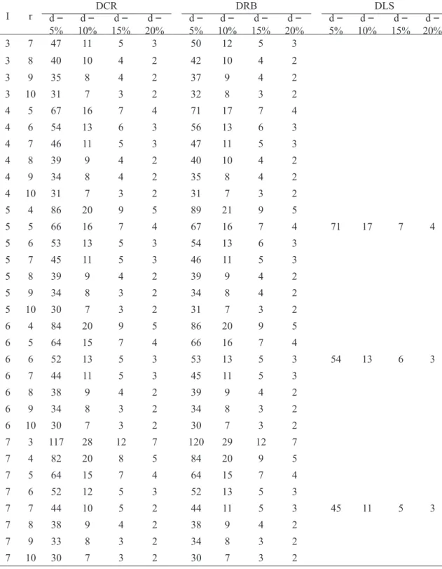
the space of the experimental area, The question that comes up is whether to increase the plot size or the number of replications. In case the researcher wants to evaluate NL of 5 treatments in a DCR, and
wishes to 15% precision, can use as options, seedling
plots with 9 and 4 replications, 7 seedlings and 5 replications, 4 seedlings and 5 replications, among others (Table 3), since, in the said experiment, each BEU corresponds to a single seedling. In the three options mentioned, the total number of seedlings per experiment would be, respectively 180, 175
and 150. Thus, it is clear that the most efficient
use of space in the nursery occurs with increasing number of replications. This same behavior was also observed by Henriques Neto et al. (2004) to wheat and, Cargnelutti Filho et al. (2014) to gray velvet
bean in field experiments.
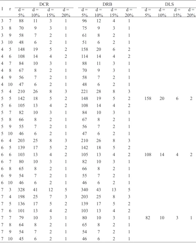
In the comparative evaluation between experimental designs for a particular character, for the same number of treatments, replications and the same precision, there is a tendency of the sample size grow in order DCR <DRB <DLS. By way of example consider the SH assessment of 5 treatments,
5 replicates and 5% precision, wherein X0 will beof 142, 148 and 158 seedlings per plot, respectively, for a DCR, DRB and DLS (Table 2). Algebraically, the difference is in the number of degrees of freedom (df) attributed to the residue, that will alter the values of t1 and t2 expression of Hatheway (1961). In the said example are 20 df to DCR, obtained by I (r – 1) = 5(5 – 1) = 20 df; 16 df for a DRB, obtained by (I – 1)(r – 1) = (5 – 1)(5 – 1) = 16 df e 12 df for a DLS, obtained by (I – 1)(I – 2) = (5 – 1)(5 – 2) = 12 df, whose values t1 will 2,086 for a DCR; 2,120
for a DRB and 2,179 for a DLS. Another finding
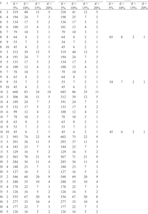
in the comparison between the designs is that, as it increases the number of treatments and replications, it also increases the number of df residue and consequently the difference of X0 decreases until no more exist. In the said example for SH with
5% precision, when it is increased to 10 treatments
and 10 replications, X0 is of 45 plants per plot for a DCR, DRB and DLS (Table 2). It explained this fact, due to alterations in Student’s t values were far smaller to high residue df values, assuming values of 1.987 for a DCR, 1.9895 for a DRB and 1.993 for a DLS. Another practical aspect of these results is that, as the seedlings are grown in nurseries, where the environment tends to be homogeneous; experimentation can be performed in a completely randomized design, with less spent seedlings in most cases.
Tables 2, 3 and 4 bring options so that one can work on developing experimental research with ‘Baixinho de Santa Amália’ guided in design
and efficiency of the use of experimental designs
completely randomized, randomized block and Latin square. However, the researcher may have the necessity to work with a number of treatments and
replications or in which scenarios is not included in this study. In this case the referred plot size can
be obtained from the coefficient of variation values
between the plots of Xi UEB of size (Table 1) and
the heterogeneity coefficient values (Figure 2) using
the equation X0 = √2(t1+t2)2 CV2/rd2 of Hatheway (1961). The Student’s t value necessary in equation can be obtained in books that contains more complete table, without the necessity of interpolation, such as Zar (2010), or directly in software such as Excel (LEVINE et al., 2012), (MATLAB, 2010) and, R (R Development Core Team, 2014), among others.
In a realistic scenarios, appointed by the variance between the experimental units according to the number of BEU (Table 1, Figure 2), it is observed that reducing the variance is very negligible with the number of BEU above of 10. The same behavior
can be verified when evaluating the coefficients
of variation between the BEU according to the different plot sizes (Table 1). Thus, the adoption of plot size above 10 require much less precision
verified in this study, which are between 10 and 20%. In fact, in all these scenarios it was detected plot size above 10 when used precision of 5%. Thus,
it is recommended that the plot size is not more than 10 seedlings. In fact if is considered a precision of
15% will be needed 9 seedlings per plot, with use
5 to 30 treatments and four replications (Table 3) in the design of randomized blocks and completely randomized design.
TABLE 1 - Size planned plot (Xi), in basic experimental units (BEU); number of plots with Xi BEU of size (n); mean plots with Xi BEU of size [ m(Xi)]; coeficiente of variation between plots of Xi BEU of size [ CV(Xi), in %]; and, varience by BEU between plots of Xi BEU of size [VU (Xi) ]. Seedling height data (SH, in cm), number of leaves per plant (NL) and the longest root length (LRL, in cm) in papaya seedlings (Carica papaya L.) cv. Baixinho de Santa Amália in a blank test with 240 BEU.
TABLE 2 - Optimal size of plots (X0), in number of seedlings per plot, estimated by method of Hatheway (1961) to experimental design in designs completely randomized (DCR), randomized blocks (DRB) and Latin square (DLS), in scenarios formed by combinations of I treatments, r
replications, and d differences between treatment means to be detected as significant at the 5% probability, expressed as a percentage of the overall mean of the experiment (precision)
for the data height papaya seedling (Carica papaya L.) cv. Baixinho de Santa Amália.
I r
DCR DRB DLS
d =
5% 10%d = 15%d = 20%d = d = 5% 10%d = 15%d = 20%d = d = 5% 10%d = 15%d = 20%d =
3 7 88 11 3 1 96 12 4 1
3 8 70 9 3 1 75 9 3 1
3 9 58 7 2 1 61 8 2 1
3 10 48 6 2 1 51 6 2 1
4 5 148 19 5 2 158 20 6 2
4 6 108 14 4 2 114 14 4 2
4 7 84 10 3 1 88 11 3 1
4 8 67 8 2 1 70 9 3 1
4 9 56 7 2 1 58 7 2 1
4 10 47 6 2 1 48 6 2 1
5 4 210 26 8 3 221 28 8 3
5 5 142 18 5 2 148 19 5 2 158 20 6 2
5 6 105 13 4 2 108 14 4 2
5 7 82 10 3 1 84 10 3 1
5 8 66 8 2 1 67 8 2 1
5 9 55 7 2 1 56 7 2 1
5 10 46 6 2 1 47 6 2 1
6 4 203 25 8 3 210 26 8 3
6 5 139 17 5 2 142 18 5 2
6 6 103 13 4 2 105 13 4 2 108 14 4 2
6 7 80 10 3 1 82 10 3 1
6 8 65 8 2 1 66 8 2 1
6 9 54 7 2 1 55 7 2 1
6 10 46 6 2 1 46 6 2 1
7 3 328 41 12 5 340 43 13 5
7 4 198 25 7 3 203 25 8 3
7 5 136 17 5 2 139 17 5 2
7 6 101 13 4 2 103 13 4 2
7 7 79 10 3 1 80 10 3 1 82 10 3 1
7 8 64 8 2 1 65 8 2 1
7 9 54 7 2 1 54 7 2 1
7 10 45 6 2 1 46 6 2 1
TABLE 2 – continuation ...
I r
DCR DRB DLS
d =
5% 10%d = 15%d = 20%d = d = 5% 10%d = 15%d = 20%d = d = 5% 10%d = 15%d = 20%d =
8 3 319 40 12 5 328 41 12 5
8 4 194 24 7 3 198 25 7 3
8 5 134 17 5 2 136 17 5 2
8 6 100 13 4 2 101 13 4 2
8 7 79 10 3 1 79 10 3 1
8 8 64 8 2 1 64 8 2 1 65 8 2 1
8 9 53 7 2 1 54 7 2 1
8 10 45 6 2 1 45 6 2 1
9 3 312 39 12 5 319 40 12 5
9 4 191 24 7 3 194 24 7 3
9 5 133 17 5 2 134 17 5 2
9 6 100 12 4 2 100 13 4 2
9 7 78 10 3 1 79 10 3 1
9 8 63 8 2 1 64 8 2 1
9 9 53 7 2 1 53 7 2 1 54 7 2 1
9 10 45 6 2 1 45 6 2 1
10 2 660 83 24 10 685 86 25 11
10 3 306 38 11 5 312 39 12 5
10 4 189 24 7 3 191 24 7 3
10 5 132 17 5 2 133 17 5 2
10 6 99 12 4 2 100 12 4 2
10 7 78 10 3 1 78 10 3 1
10 8 63 8 2 1 63 8 2 1
10 9 53 7 2 1 53 7 2 1
10 10 45 6 2 1 45 6 2 1 45 6 2 1
15 2 593 74 22 9 602 75 22 9
15 3 291 36 11 5 293 37 11 5
15 4 183 23 7 3 184 23 7 3
15 5 129 16 5 2 129 16 5 2
20 2 563 70 21 9 567 71 21 9
20 3 284 36 11 4 285 36 11 4
20 4 180 23 7 3 180 23 7 3
20 5 127 16 5 2 127 16 5 2
25 2 546 68 20 9 548 69 20 9
25 3 280 35 10 4 280 35 10 4
25 4 178 22 7 3 178 22 7 3
25 5 126 16 5 2 126 16 5 2
30 2 535 67 20 8 536 67 20 8
30 3 277 35 10 4 277 35 10 4
30 4 177 22 7 3 177 22 7 3
TABLE 3 - Optimal size of plots (X0), in number of seedlings per plot, estimated by method of Hatheway (1961) to experimental design in designs completely randomized (DCR), randomized blocks (DRB) and Latin square (DLS), in scenarios formed by combinations of I treatments, r
replications, and d differences between treatment means to be detected as significant at the 5%
probability, expressed as a percentage of the overall mean of the experiment (precision) for the data number of leaves for papaya seedlings (Carica papaya L.) cv. Baixinho de Santa Amália
I r
DCR DRB DLS
d =
5% 10%d = 15%d = 20%d = d = 5% 10%d = 15%d = 20%d = d = 5% 10%d = 15%d = 20%d =
3 7 47 11 5 3 50 12 5 3
3 8 40 10 4 2 42 10 4 2
3 9 35 8 4 2 37 9 4 2
3 10 31 7 3 2 32 8 3 2
4 5 67 16 7 4 71 17 7 4
4 6 54 13 6 3 56 13 6 3
4 7 46 11 5 3 47 11 5 3
4 8 39 9 4 2 40 10 4 2
4 9 34 8 4 2 35 8 4 2
4 10 31 7 3 2 31 7 3 2
5 4 86 20 9 5 89 21 9 5
5 5 66 16 7 4 67 16 7 4 71 17 7 4
5 6 53 13 5 3 54 13 6 3
5 7 45 11 5 3 46 11 5 3
5 8 39 9 4 2 39 9 4 2
5 9 34 8 3 2 34 8 4 2
5 10 30 7 3 2 31 7 3 2
6 4 84 20 9 5 86 20 9 5
6 5 64 15 7 4 66 16 7 4
6 6 52 13 5 3 53 13 5 3 54 13 6 3
6 7 44 11 5 3 45 11 5 3
6 8 38 9 4 2 39 9 4 2
6 9 34 8 3 2 34 8 3 2
6 10 30 7 3 2 30 7 3 2
7 3 117 28 12 7 120 29 12 7
7 4 82 20 8 5 84 20 9 5
7 5 64 15 7 4 64 15 7 4
7 6 52 12 5 3 52 13 5 3
7 7 44 10 5 2 44 11 5 3 45 11 5 3
7 8 38 9 4 2 38 9 4 2
7 9 33 8 3 2 34 8 3 2
7 10 30 7 3 2 30 7 3 2
TABLE 3 – continuation ...
I r
DCR DRB DLS
d =
5% 10%d = 15%d = 20%d = d = 5% 10%d = 15%d = 20%d = d = 5% 10%d = 15%d = 20%d =
8 3 114 27 12 7 117 28 12 7
8 4 81 19 8 5 82 20 8 5
8 5 63 15 7 4 64 15 7 4
8 6 52 12 5 3 52 12 5 3
8 7 44 10 4 2 44 10 5 2
8 8 38 9 4 2 38 9 4 2 38 9 4 2
8 9 33 8 3 2 33 8 3 2
8 10 30 7 3 2 30 7 3 2
9 3 113 27 12 6 114 27 12 7
9 4 80 19 8 5 81 19 8 5
9 5 63 15 6 4 63 15 7 4
9 6 51 12 5 3 52 12 5 3
9 7 43 10 4 2 44 10 4 2
9 8 38 9 4 2 38 9 4 2
9 9 33 8 3 2 33 8 3 2 33 8 3 2
9 10 30 7 3 2 30 7 3 2
10 2 189 45 19 11 194 46 20 11
10 3 111 27 11 6 113 27 12 6
10 4 80 19 8 5 80 19 8 5
10 5 62 15 6 4 63 15 6 4
10 6 51 12 5 3 51 12 5 3
10 7 43 10 4 2 43 10 4 2
10 8 37 9 4 2 38 9 4 2
10 9 33 8 3 2 33 8 3 2
10 10 30 7 3 2 30 7 3 2 30 7 3 2
15 2 176 42 18 10 177 42 18 10
15 3 107 26 11 6 108 26 11 6
15 4 78 19 8 4 78 19 8 4
15 5 61 15 6 3 61 15 6 3
20 2 169 40 17 10 170 41 18 10
20 3 106 25 11 6 106 25 11 6
20 4 77 18 8 4 77 18 8 4
20 5 61 14 6 3 61 14 6 3
25 2 166 40 17 9 166 40 17 9
25 3 105 25 11 6 105 25 11 6
25 4 77 18 8 4 77 18 8 4
25 5 60 14 6 3 60 14 6 3
30 2 163 39 17 9 164 39 17 9
30 3 104 25 11 6 104 25 11 6
30 4 76 18 8 4 76 18 8 4
TABLE 4 - Optimal size of plots (X0), in number of seedlings per plot, estimated by method of Hatheway (1961) to experimental design in designs completely randomized (DCR), randomized blocks (DRB) and Latin square (DLS), in scenarios formed by combinations of I treatments, r
replications, and d differences between treatment means to be detected as significant at the 5% probability, expressed as a percentage of the overall mean of the experiment (precision),
for the data length of the longest root papaya seedlings (Carica papaya L.) cv. Baixinho de Santa Amália
I r
DCR DRB DLS
d =
5% 10%d = 15%d = 20%d = 5%d = 10%d = 15%d = 20%d = 5%d = 10%d = 15%d = 20%d =
3 7 35 8 4 2 37 9 4 2
3 8 30 7 3 2 31 8 3 2
3 9 26 6 3 2 27 7 3 2
3 10 23 6 2 1 24 6 3 1
4 5 50 12 5 3 52 13 5 3
4 6 40 10 4 2 42 10 4 2
4 7 34 8 4 2 35 8 4 2
4 8 29 7 3 2 30 7 3 2
4 9 26 6 3 1 26 6 3 2
4 10 23 5 2 1 23 6 2 1
5 4 64 15 7 4 66 16 7 4
5 5 49 12 5 3 50 12 5 3 52 13 5 3
5 6 40 10 4 2 40 10 4 2
5 7 33 8 3 2 34 8 4 2
5 8 29 7 3 2 29 7 3 2
5 9 25 6 3 1 26 6 3 1
5 10 23 5 2 1 23 5 2 1
6 4 62 15 6 4 64 15 7 4
6 5 48 12 5 3 49 12 5 3
6 6 39 9 4 2 40 10 4 2 40 10 4 2
6 7 33 8 3 2 33 8 3 2
6 8 28 7 3 2 29 7 3 2
6 9 25 6 3 1 25 6 3 1
6 10 22 5 2 1 23 5 2 1
7 3 86 21 9 5 89 21 9 5
7 4 61 15 6 4 62 15 6 4
7 5 47 11 5 3 48 12 5 3
7 6 39 9 4 2 39 9 4 2
7 7 33 8 3 2 33 8 3 2 33 8 3 2
7 8 28 7 3 2 28 7 3 2
7 9 25 6 3 1 25 6 3 1
TABLE 4 – continuation ...
I r
DCR DRB DLS
d =
5% 10%d = 15%d = 20%d = d = 5% 10%d = 15%d = 20%d = d = 5% 10%d = 15%d = 20%d =
8 3 85 20 9 5 86 21 9 5
8 4 60 14 6 3 61 15 6 4
8 5 47 11 5 3 47 11 5 3
8 6 38 9 4 2 39 9 4 2
8 7 32 8 3 2 33 8 3 2
8 8 28 7 3 2 28 7 3 2 28 7 3 2
8 9 25 6 3 1 25 6 3 1
8 10 22 5 2 1 22 5 2 1
9 3 83 20 9 5 85 20 9 5
9 4 60 14 6 3 60 14 6 3
9 5 47 11 5 3 47 11 5 3
9 6 38 9 4 2 38 9 4 2
9 7 32 8 3 2 32 8 3 2
9 8 28 7 3 2 28 7 3 2
9 9 25 6 3 1 25 6 3 1 25 6 3 1
9 10 22 5 2 1 22 5 2 1
10 2 139 34 15 8 143 34 15 8
10 3 82 20 9 5 83 20 9 5
10 4 59 14 6 3 60 14 6 3
10 5 46 11 5 3 47 11 5 3
10 6 38 9 4 2 38 9 4 2
10 7 32 8 3 2 32 8 3 2
10 8 28 7 3 2 28 7 3 2
10 9 25 6 3 1 25 6 3 1
10 10 22 5 2 1 22 5 2 1 22 5 2 1
15 2 130 31 14 7 131 31 14 8
15 3 80 19 8 5 80 19 8 5
15 4 58 14 6 3 58 14 6 3
15 5 45 11 5 3 46 11 5 3
20 2 125 30 13 7 126 30 13 7
20 3 78 19 8 5 78 19 8 5
20 4 57 14 6 3 57 14 6 3
20 5 45 11 5 3 45 11 5 3
25 2 122 29 13 7 123 30 13 7
25 3 77 19 8 4 78 19 8 4
25 4 57 14 6 3 57 14 6 3
25 5 45 11 5 3 45 11 5 3
30 2 121 29 13 7 121 29 13 7
30 3 77 18 8 4 77 19 8 4
30 4 57 14 6 3 57 14 6 3
CONCLUSIONS
In the comparison between experimental designs, the plot size is greater in the Latin square, followed by a randomized block design and completely randomized, and this difference is more pronounced the lower the number of treatments and replicates used.
For the same number of treatments and
the same precision, the most efficient use of the
experimental area is given using smaller plot, with more replications, which require less space in the nursery than larger plots with fewer replications.
For experiments completely randomized and
randomized blocks with five or more treatments and
four or more replications, it is recommended to use nine seedlings per plot of ‘Baixinho de Santa Amália’
in nurseries, corresponding precision to 15% of the
mean.
ACKNOWLEDGEMENTS
T h e a u t h o r s t h a n k C o o r d e n a ç ã o d e Aperfeiçoamento de Pessoal de Nível Superior (CAPES) by the grant of scholarships and to Caliman agrícola S/A for the supply of seeds for the research.
REFERENCES
BRITO, M.C.M.; FARIA, G.A.; MORAIS, A.R.; SOUZA, E.M.; DANTAS, J.L.L. Estimação do tamanho ótimo de parcela via regressão antitônica.
Revista Brasileira Biometria, São Paulo, v.30, n.3, p.353-366, 2012. Disponível em: <http://jaguar.fcav. unesp.br/RME/fasciculos/v30/v30_n3/A4_Marcio. pdf>.
BRITO, M.C.M.; HUMADA-GONZÁLEZ, G.G.; MORAIS, A.R. de; MOREIRA, J.M. Avaliação do desempenho do algoritmo de reamostragem
bootstrap na verificação da estimação do tamanho
ótimo da parcela. Revista da Estatística UFOP, Ouro Preto, v.3, n.3, p.255-259, 2014. Disponível em: <http://www.cead.ufop.br/jornal/index.php/rest/ article/view/577/481>.
CARGNELUTTI FILHO, A.; TOEBE, M.; ALVES, B.M.; BURIN, C.; NEU, I.M.; FACCO, G. Tamanho amostral para avaliar a massa de plantas de mucuna cinza. Comunicata Scientiae, João Pessoa, v.5, n.2, p.196-204, 2014. Disponível em: <http:// comunicata.ufpi.br/index.php/comunicata/article/ view/328/245>.
CIPRIANO, P.E.; COGO, F.D.; CAMPOS, K.A.;
ALMEIDA, S.L.S de. Suficiência amostral para mudas
de cafeeiro cv. Rubi. Revista Agrogeoambiental, Pouso Alegre, v.4, n.1, p.61-66, 2012. Disponível em: <http://agrogeoambiental.ifsuldeminas.edu.br/ index.php/Agrogeoambiental/article/view/375/371>.
FIRMINO, R.A.; COGO, F.D.; ALMEIDA, S.L.S.; CAMPOS, K.A.; MORAIS, A.R.Tamanho ótimo de parcela para experimentos com mudas de café Catuai Amarelo 2SL. Revista Tecnologia e Ciência Agropecuária, João Pessoa, v.6, n.1, p.9-12, 2012. Disponível em: <http://www.emepa.org.br/revista/ volumes/tca_v6_n1_mar/tca6102.pdf>.
HATHEWAY, W.H. Convenient plot size. Agronomy
Journal, Madison, v.53, n.4, p.279-280, 1961.
HENRIQUES NETO, D.; SEDIYAMA, T.; SOUZA, M.A. de; CECON, P.R.; YAMANAKA, C.H.; SEDIYAMA, M.A.N.; VIANA, A.E.S. Tamanho de parcelas em experimentos com trigo irrigado
sob plantio direto e convencional. Pesquisa
Agropecuária Brasileira, Brasília, v.39, n.6, p.517-524, 2004. Disponível em: <http://www.scielo.br/ pdf/pab/v39n6/v39n6a01>.
LEONARDO, F.A.P.; PEREIRA, W.E.; SILVA, S.M.; ARAÚJO, R.C.; MENDONÇA, R.M.N. Tamanho ótimo da parcela experimental de abacaxizeiro ‘Vitória’. Revista Brasileira de Fruticultura, Jaboticabal, v.36, n.4, p.909-916, 2014. Disponível em: <http://www.scielo.br/pdf/rbf/v36n4/a18v36n4. pdf >.
LEVINE, D.M.; STEPHAN, D.F.; KREHBIEL, T.C.; BERENSON, M.L. Estatística: teoria e aplicações usando Microsoft Excel em português. 6.ed. Rio de Janeiro: LTC Editora, 2012. 832p.
LORENTZ, L.H.; ERICHSEN, R.; LÚCIO, A.D. Proposta de método para estimação de tamanho de parcela para culturas agrícolas. Revista Ceres, Viçosa, MG, v.59, n.6, p.772-780, 2012. Disponível em: <http://www.scielo.br/pdf/rceres/v59n6/06. pdf >.
MEIER, V.D.; LESSMAN, K.J. Estimation of optimum Field plot shape and size for testing yield in
Crambe abyssinica Hochst. Crop Science, Madison, v.11, n.5, p.648-650, 1971. Disponível em: <https:// www.crops.org/publications/cs/abstracts/11/5/CS01 10050648?access=0&view=pdf>.
MELO, A.S.; COSTA, C.X.; BRITO, M.E.B.; VIÉGAS, P.R.A.; SILVA JUNIOR, C.D. Produção de mudas de mamoeiro em diferentes substratos e doses de fósforo. Revista Brasileira de Ciências Agrárias, Recife, v.2, n.4, p.257-261, 2007. Disponível em: <http://www.agraria.pro.br/sistema/ index.php?journal=agraria&page=article&op=view &path[]=148&path[]=111>.
MENGARDA, L.H.G.; LOPES, J.C.; BUFFON, R.B. Emergência e vigor de mudas de genótipos
de mamoeiro em função da irradiância. Pesquisa
Agropecuária Tropical, Goiânia, v.44, n.3, p.325-333, 2014. Disponível em: <http://www.redalyc.org/ pdf/2530/253032129011.pdf>.
MORAIS, A.R. de; ARAÚJO, A.G. de; PASQUAL, M.; PEIXOTO, A.P.B. Estimação do tamanho de parcela para experimento com cultura de tecidos em videira. Semina: Ciências Agrárias, Londrina, v.35, n.1, p.113-124, 2014. Disponível em: <http://www. uel.br/revistas/uel/index.php/semagrarias/article/ view/12579/pdf_216>.
OLIVEIRA FILHO, F.S.; HAFLE, O.M.; ABRANTE, E.G.; OLIVEIRA, F.T.; SANTOS, V.M. Produção de mudas de mamoeiro em tubetes com diferentes fontes e doses de adubos orgânicos. Revista Verde de Agroecologia e Desenvolvimento Sustentável, Pombal, v.8, n.3, p.96-103, 2013. Disponível em: <http://www.gvaa.com.br/revista/index.php/ RVADS/article/view/2269/pdf_747>.
PAIXÃO, M.V.S.; SCHMILDT, E.R.; MATTIELLO, H.N.; FERREGUETTI, G.A.; ALEXANDRE, R.S. Frações orgânicas e mineral da produção de mudas de mamoeiro. Revista Brasileira de Fruticultura, Jaboticabal, v.34, n.4, p.1105-1112, 2012. Disponível em: <http://www.scielo.br/pdf/rbf/v34n4/18.pdf>.
PARANAÍBA, P.F.; FERREIRA, D.F.; MORAIS, A.R. Tamanho ótimo de parcelas experimentais:
proposição de métodos de estimação. Revista
Brasileira de Biometria, São Paulo, v.27, n.2, p.255-268, 2009. Disponível em: <http://jaguar.fcav.unesp. br/RME/fasciculos/v27/v27_n2/Patricia.pdf>.
PEIXOTO, A.P.B.; FARIA, G.A.; MORAIS, A.R. Modelos de regressão com platô na estimativa do tamanho de parcelas em experimento de conservação
in vitro de maracujazeiro. Ciência Rural, Santa Maria, v.41, n.11, 1907-1913, 2011. Disponível em: <http://www.scielo.br/pdf/cr/v41n11/a16711cr4630. pdf>.
PIMENTEL-GOMES, F. Curso de estatística
experimental. 15.ed. Piracicaba: Fealq, 2009. 451p.
R Core Team. R: a language and environment for statistical computing. Vienna: R Foundation for Statistical Computing. 2014. Disponível em: <http:// www.R-project.org/>. Acesso em: 4 dez. 2014.
SÁ, F.V.S.; BRITO, M.E.B.; MELO A.S.; ANTÔNIO NETO, P.; FERNANDES, P.O.D.; FERREIRA, I.B. Produção de mudas de mamoeiro irrigadas com
água salina. Revista Brasileira de Engenharia
Agrícola e Ambiental, Campina Grande, v.17, n.10, p.1047–1054, 2013. Disponível em: <http://www. scielo.br/pdf/rbeaa/v17n10/04.pdf>.
S E R R A N O , L . A . L . ; C AT TA N E O , L . F. ; FERREGUETTI, G.A. Adubo de liberação lenta na produção de mudas de mamoeiro. Revista Brasileira de Fruticultura, Jaboticabal, v.32, n.3, p.874-883, 2010. Disponível em: <http://www.scielo.br/pdf/rbf/ v32n3/aop09010.pdf>.
SMITH, H.F. An empirical law describing heterogeneity in the yields of agricultural crops. The Journal of Agricultural Science, Cambridge,v.28, n.1, p.1-23, 1938. Disponível em: <http://journals. cambridge.org/action/displayAbstract?fromPage=o
nline&aid=4689276&fileId=S0021859600050516>.
STEEL, R.G.D.; TORRIE, J.H.; DICKEY, D.A.
Principles and procedures of statistics: a biometrical approach. 3rd ed. New York: MacGraw-Hill Book Companies, 1997. 666p.
STORCK, L.; GARCIA, D.C.; LOPES, S.J.;
ESTEFANEL, V. Experimentação vegetal. 3.ed.
Santa Maria: UFSM, 2011. 198p.
![TABLE 1 - Size planned plot (X i ), in basic experimental units (BEU); number of plots with X i BEU of size (n); mean plots with X i BEU of size [ m(Xi) ]; coeficiente of variation between plots of Xi BEU of size [ CV(Xi) , in %]; and, varience by BEU](https://thumb-eu.123doks.com/thumbv2/123dok_br/15882171.667356/6.765.50.682.226.557/table-size-planned-experimental-number-coeficiente-variation-varience.webp)

![FIGURE 2 - Graphical representation of the relation between the variance per basic experimental unit (BEU) between plots of X i BEU of size [VU (Xi) ] and the size of plots planned BEU and, estimates of function parameters VU (Xi) = V1(X i ) -b of Smi](https://thumb-eu.123doks.com/thumbv2/123dok_br/15882171.667356/13.765.152.660.80.962/graphical-representation-relation-variance-experimental-estimates-function-parameters.webp)
