ECODOURO - Modelling the effect of freshwater reduction and pulse discharge on the water dynamics and processes of the Crestuma Reservoir

Texto

(1)PROJECTOS DE INVESTIGAÇÃO CIENTÍFICA E DESENVOLVIMENTO TECNOLÓGICO. RELATÓRIO FINAL Relatório de Execução Material. REFERÊNCIA DO PROJECTO Nº POCTI/MGS/45533/2002. União Europeia – Fundos Estruturais. Governo da República Portuguesa.

(2) Data de Entrada_____________________ Nº de Registo ______________________. Data de Verificação__________________ Assinatura ________________________. Espaço reservado à Fundação para a Ciência e a Tecnologia. Referência do projecto: POCTI/MGS/45533/2002 Título do projecto: ECODOURO - Modelling the effect of freshwater reduction and pulse discharge on the water dynamics and processes of the Crestuma Reservoir Data de Início do Projecto: __15__/______MAR_______/_____2003__ Duração: ____36__ Meses. Prorrogado até: __15__/____SEP________/_____2006_. Data de Conclusão do Projecto: __20__/_____DEC_______/_____2006. Identificação da instituição proponente. Nome ou designação social: Centro de Investigação Marinha e Ambiental - CIIMAR Morada Rua do Campo Alegre, 823 Localidade Porto Telefone 22 608 04 70 / 71. Código postal 4150-180 Porto Fax 22 608 04 79. Email cimar@cimar.org. Unidade responsável pela execução do projecto Nome Laboratório de Hidrobiologia - ICBAS Morada Largo Abel Salazar, 2 Localidade Porto Telefone 22206285. Código postal 4099-003 Porto Fax 222062284. Email. Identificação do investigador responsável Nome Adriano Agostinho Donas Bôto Bordalo e Sá Telefone 222062285. Fax 222062284. Email bordalo@icbas.up.pt.

(3) Centro de Investigação Marinha e Ambiental Universidade do Porto Laboratório de Hidrobiologia. ECODOURO - Modelling the effect of freshwater reduction and pulse discharge on the water dynamics and processes of the Crestuma Reservoir POCTI/MGS/45533/2002. Final Report Prepared by: Adriano A. Bordalo e Sá (PI), Pedro Duarte and William Wiebe. Porto,March 2007.

(4) 1. Executive summary This report deals with the activities carried out during the project 72 months, from March 15, 2003 to September 15, 2006 under the framework of the ECODOURO - Modelling the effect of freshwater reduction and pulse discharge on the water dynamics and processes of the Crestuma Reservoir (POCTI/MGS/45533/2002). The report includes the fieldwork, data interpretation and mathematical modeling according to the seven working packages presented in the original proposal. Data is available to the public at http://ecodouro.icbas.up.pt. The main objectives of this goal oriented research project implemented on the Crestuma Reservoir (Douro River) are: i. To evaluate the long-term effects of flow reduction on key environmental variables and processes that occur in the Crestuma Reservoir; and ii. To evaluate the effect of high frequency oscillations (freshwater pulse discharges) on the ecosystem dynamics in terms of water column stratification, water temperature and turbidity, oxygen, nutrient availability, phytoplankton biomass and primary productivity. The original requested budget was reduced by 19%, and the evaluation commission recommended the non-acquisition of a second multiprobe CTD. Thus, the entire field survey program was changed accordingly. The seasonal sampling was conducted at two anchor stations located about 500 m and 2,500 m from the Crestuma dam crest. Surveys were performed on December 2003 (Fall), February 2004 (Winter), May 2004 (Spring) and August 2004 (Summer). An un-scheduled survey was carried out at the onset of the program (May 2003), in order to gather basic data since no departure data (short term series) were available contrarily to what was though. This approach proved to be very useful and the obtained results were applied in the following surveys. Moreover, since no workable bathymetrics were available to the research team (only depth contours in chart format restricted to the navigational channel) several dedicated surveys were organized in order to generate bottom contour maps for the last 10 km of the reservoir, covering the two-field stations location. As a result, a costume-made GIS was created and data used to run the model. All technical details of both the employed models (2D-vertically resolved model and the coupled biogeochemical model), including the complete mathematical formulae, are 1.

(5) presented in Annexes I and II. The rationale for selection of the modeled parameters are presented; the field data obtained from the 4+1 surveys were used to initialize the models. It was found that the different flow time-scales might influence water dynamics, biogeochemistry and primary productivity. For example, during the day, longitudinal flows results from upstream forcing, with river water entering into the reservoir. A clear longitudinal flow profile emergeed, disturbed in some points by depth changes that forces upwelling of bottom water. During the night, in the absence of river flow, at it happens frequently in Spring through Fall, convective flow dominated, with surface cooled water sinking to the bottom and forcing the ascent of bottom water. Vertical flows may be larger than horizontal ones. On the other hand, the highest phytoplankton production was observed in May and September, when microalgae were using more efficiently the available light. Furthermore, phytoplankton efficiency decreased from morning to dawn. Considering the objectives of this project, several model simulations were carried out to analyze the effects of flow variability on water column stratification and quality (cf. – Annexe III). These simulations were carried out with the same average flow magnitude and forcing conditions, in terms of water temperature, nutrients and chlorophyll concentrations, but different flow frequencies and amplitudes. Results obtained suggest that flow variability may not have a large effect on water temperature, nutrient and chlorophyll concentration and net primary production at annual time scales. However, when the time scale under analysis is reduced to seasonal and monthly, effects of flow variability become apparent, especially during the summer period and when flow is hold constant. Constant flow implies that extreme low and high values do not occur. Under this situation of “extreme” flow regulation, it appears that the synergies between river forcing and reservoir processes tend to reduce phytoplankton biomass. Therefore, from a management point of view, it is apparent that stabilizing the flow may prevent the development of phytoplankton blooms. On the other hand, results presented and discussed in Annex IV suggest that the Crestuma reservoir has undergone some important changes over the period 1999-2005, with significant increases in nitrogen and phosphorus and a decrease in the nitrogen: phosphorus ratio i.e. the Redfield ratio. One possible change, arising from the shifts in the nitrogen: phosphorus ratio, is the apparent autumn shift towards nitrate-nitrogen limitation of phytoplankton. Apart from increasing nutrient runoff within the watershed, the 2.

(6) noticeable nutrient increase trend found in the Crestuma resevoir may also be explained by the reduction of chlorophyll as a result of the massive development of the invasive clam Corbicula sp. Thus, the Crestuma reservoir is now a predominantly heterotrophic ecosystem that is the source of water to 20% of the Portuguese population and feeds the Douro estuary with most of the water that reaches the Atlantic Ocean.. As a result of this project, a full functional calibrated with dedicated data model is available. During the 72 mo of the project, three young researchers were able to work and get training in the different areas covered by the program. Due to the enormous amount of data gathered, only two research papers were published. Thus, in the near future, two papers will be submitted (as a result of Annex III and Annex IV), and two additional papers are under preparation. Part of the obtained data has being used for teaching purposes at undergraduate and Master/PhD levels by the PI and the Cemas team.. 3.

(7) 2. Introduction The Douro River flows within the largest watershed in the Iberian Peninsula, draining 98,000 km2 or 17% of this territory. The Douro is an international watershed, shared between Spain (80%) and Portugal (20%). Within the watershed, 51 large dams regulate the flow, allowing, presently, about 15 km3 of freshwater per year to be discharged into the Atlantic Ocean at 41º08’N; 08º41’W, an equivalent to 455 m3s-1. However, because the flow regime depends not only on climatic conditions but also is controlled for hydroelectric power generation needs in both countries, as well as by irrigation needs in Spain, the daily discharge rate into the ocean ranges between zero and >13,000 m3s-1 (Vieira and Bordalo 2000). The first dam on the watershed was built in 1920, but most large dams (>15m wall height) started operating in the late 1950s. The concentration of dams is particularly heavy in the last 350 km of the river main course, with a hydroelectric power dam about every 30 km. Altogether, the large dams retain up to 1100 hm3 (13%) of water in Portuguese reservoirs and 7500 hm3 (87%) on the Spanish side of the watershed. The scientific evaluation of the water quality, and its temporal trends, is an important task for risk assessment. This is particularly critical when dealing with an international river, i.e., a shared watershed, because the management goals of the different countries may not coincide. The main objectives of this goal oriented research project implemented on the Crestuma Reservoir (Douro River) are: i.. To evaluate the long term effects of flow reduction on key environmental variables and processes that occur in the Crestuma Reservoir;. ii.. To evaluate the effect of high frequency oscillations (freshwater pulse discharges) on the ecosystem dynamics in terms of water column stratification, water temperature and turbidity, oxygen, nutrient availability, phytoplankton biomass and primary productivity.. In order to achieve the above stated objectives, a 2-D vertically resolved coupled physicalbiogeochemical model, based on an object-oriented ecological approach, was implemented.. 4.

(8) The present final progress report deals with the activities carried out during the project 72 months, from March 15, 2003 to September 15, 2006.. 3. Selection of BIC researchers In April 2003 two vacancies for BIC fellowships associated to ECODOURO were advertised. By April 10, 19 candidacies were received and on May 7, interviews of 18 candidates were conducted. Two candidates were selected: for BIC1 – Rita Teixeira and for BIC2 - Claudia Martins. The BIC1 is based at Laboratório de Hidrobiologia ICBAS/CIIMAR (Prime Contractor) and BIC2 at CEMAS (second project partner). BIC1 started working on May 15, 2003 and BIC2 on July 25, 2003. BIC1 was initially awarded for 18 mo but, with permission from FCT, was extended until the end of the project (36 mo). By December 2004 BIC2 left the research team. Thus, in February 2005, a BIC fellowship associated with ECODOURO was advertised, to replace the BIC2 grant given previously to CEMAS (second project partner). By March 31, 57 proposals were received, 17 were selected for interview. Of these, only 12 candidates showed-up and were interviewed. One candidate was selected - Cátia Rabaça. The selected candidate started working in May 2005. By October 2005 BIC2 also left the research team.. 4. Funding From the original budget of 125 266€ requested to FCT, only 105 266€ were made available, according to the evaluation panel. Thus, a 20 000€ stake (initially allocated for the purchase of a multiprobe CTD) was not considered. The budget was reformulated and sent to FCT on March 15, 2003. However, the first installment was made available to the Prime Contractor only on September 1, 2003, followed by two additional installments (Table 1.1).. 5.

(9) Table 1.1. Listing of installments from FCT and from Ciimar to Cemas.. 5. Work Plan According to the original proposal submitted on May 25, 2002, ECODOURO is divided into seven Work Packages (WP) as follows: i.. WP1 – Data gathering and organization;. ii.. WP2 – Seasonal sampling surveys;. iii.. WP3 – Time-series analysis;. iv.. WP4 – Implementation of a 2D vertically resolved model;. v.. WP5 – Model calibration and validation;. vi.. WP6 – Data analysis and reporting;. vii.. WP7 – Web page.. Due to the budget reduction, some changes were introduced, namely on WP2. The unavailability of the second multiprobe logger, which purchased was jugged unnecessary by the evaluation panel, resulted in the impossibility to perform water column mass balance of key environmental parameters, namely temperature, conductivity, dissolved oxygen, pH and turbidity according to the original plan.. 6.

(10) WP1 – Data gathering and organization The work planned for 3 mo was completed. The database was organized in Excel, as originally proposed. It consists of historic surface water physical and chemical data from the Portuguese Water Institute - Ministry of Environment (www.inag.pt) for three locations within the Crestuma Reservoir, namely Crestuma (1988 - 2001), Melres (1993 – 2002) and Entre-os-Rios (1993 – 2000). Also, physical and chemical data from the Porto Water Board was obtained, for a single water column station located about 1 km from the dam, covering the period 1989 – 1997. Our own data set, of monthly surveys carried out in 15 stations located in the last 30 km of the reservoir, from June 2000 to May 2001 was made available, as well as monthly (1933 – 2005), daily (1955 – 2005) and hourly (selected dates) of freshwater discharge. The main drawback of using the above mentioned third party physical and chemical databases is the lack of control over sampling and laboratory treatment the samples, as well as the existence of blanks over the considered period, either of individual parameters for one to several months (e.g. temperature and pH) as well as the discontinuation of selected parameters (phytoplankton, etc), reducing dramatically the scientific usefulness of the data. Nevertheless, and because the Crestuma INAG survey station is a rather long data-set, it was possible to identify trends, at least as yearly averages, in key environmental parameters, such as nutrients. In order to characterize the quality of the Portuguese side of the watershed, useful for the understanding of the water quality dynamics of the Crestuma Reservoir, data for two additional upstream reservoirs were also obtained from the INAG website (www.inag.pt). After a suitable data treatment, namely through the application of a water quality index, a research paper was published in an international journal (Bordalo et al 2006).. WP2 – Seasonal sampling surveys This Work Package was reformulated, in order to increase the amount of data to be obtained, following the analysis and interpretation of the above mentioned data basis, specially our own. The 12 h seasonal surveys were transformed into 25 h seasonal surveys and the seasonal weekly surveys performed during 5 days, at only one station, 7.

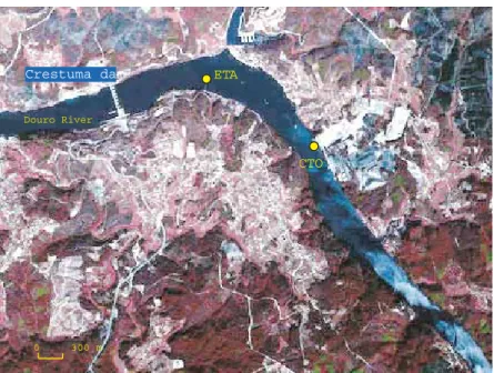
(11) due to the lack of power/logging autonomy of the existing CTDs since only one new CTD was purchased as mentioned above Moreover, an unscheduled preliminary seasonal survey was organized in May 2003 in order to gather time-series data in a single sampling station. Two 25 h sub-surveys were carried out on Sunday, May 23 and Wednesday, May 26. This corresponded roughly to periods of artificially reduced flow (Sunday), due to the modest needs in hydroelectric power generation, and to “regular” flow (Wednesday) for that period of the year. It should be noted that the fieldwork started in May, well before the first installment was received (see #4). Further seasonal surveys were organized between 7 – 10 December 2003 (Fall), 15 – 18 February 2004 (Winter), 23-27 May 2004 (Spring), 31 August – 6 September 2004 (Summer).. May 2003 survey The anchor station was located 2.5 km upstream the dam crest, at the premises of the Turbogás Tapada do Outeiro Power Plant (CTO) (Figure WP1.2), a private company that kindly gave the necessary permit for the use of the facilities. Three CTDs were installed at surface, 5 m and near bottom. Temperature, conductivity, dissolved oxygen, oxygen saturation, pH and turbidity data were obtained at 5 min intervals. Since only one CDT with a chlorophyll sensor was purchased (the second was considered non-essential by the evaluation team), continuous record of chlorophyll data was possible only at surface. A subsurface current meter gathered water velocity data and flow direction also at 5 min intervals. Every three hours, surface water samples were retrieved for nutrients, phytoplankton biomass (chlorophyll a), community respiration and primary productivity. At 15 min intervals, photosynthetic active radiation was recorded, and every 3 h, water column light profiles were obtained. Water transparency was also evaluated from Secchi disk measurements. Samples were processed immediately in a field laboratory installed on location, equipped with all required equipment and materials (Figure WP2.2). Wastes (especially toxic and/or radioactive liquid effluents) were disposed according to good laboratory practice.. 8.

(12) Crestuma dam. ETA. Douro River. CTO. 0. 300 m. Figure WP1.2. Location of the sampling stations in Crestuma reservoir (ETA - downstream; CTO – upstream).. December 2003 - fall survey Two anchor stations were established. The first, CTO, was described above (Figure WP2.2). The second (ETA), was located at the surface water treatment plant of the public company Águas do Douro e Paiva (ADP) about 500 m from the dam crest. It should also be noted the support of ADP for this project by allowing assess to their premises. At each location, two CTDs and one current meter were deployed, respectively at surface/near bottom, and at subsurface. Since only one CTD with a chlorophyll sensor was purchased as mentioned, continuous record of chlorophyll data was possible only at the CTO station (Figure WP3.2). Additionally, every three hours, surface water samples were retrieved for nutrients, phytoplankton biomass (chlorophyll a), community respiration, BOD5, primary productivity and direct bacterial counts on December 7-8 and December 10-11, for 25 h. Samples were processed immediately in the field laboratory (Figure WP4.2). At 15 min intervals, photosynthetic active radiation was recorded, and every 3 h, water column light profiles were obtained. Water transparency was also evaluated from Secchi disk measurements.. 9.

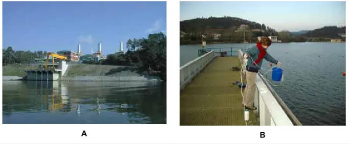
(13) A. B. Figure WP2.2. Views of CTO (A) and ETA (B) sampling stations in the Crestuma reservoir.. Figure WP3.2. Example of continuous 25-h chlorophyll a record (5 min intervals) and every 3-h measurements using the spectrophotometric method at CTO station (Fall survey).. 10.

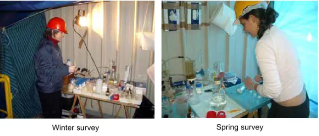
(14) February 2004 – winter survey The anchor stations were established at the above-mentioned CTO and ETA locations. At each location, two CTDs and one current meter were deployed, respectively at surface/near bottom, and at subsurface. Every three hours, surface water samples were retrieved for nutrients, phytoplankton biomass (chlorophyll a), community respiration, BOD5, primary productivity and direct bacterial counts on February 15-16 and February 18-19, for 25 h. Samples were processed immediately in the field laboratory installed at the CTO station (Figure WP4.2). At 15 min intervals, photosynthetic active radiation was recorded, and every 3 h, water column light profiles were obtained. Water transparency was also evaluated from Secchi disk measurements.. Winter survey. Spring survey. Figure WP4.2. Field laboratory installed at the Turbogás Power Plant by the Crestuma reservoir.. May 2004 - spring survey According to the original schedule, the spring surveys were performed between 23 - 27 May. The same two anchor stations were established and equipment was deployed at CTO and ETA stations as stated above. An example of surface and near bottom measurements of dissolved oxygen, pH and temperature at CTO stations is presented in Figure WP5.2.. 11.

(15) 5:30. 2:10. 22:50. 19:30. 16:10. 12:50. 9:30. 6:10. 2:50. 23:30. 20:10. 8.25 t(ºC). 8.50. 8.40. 8.30. 8.20. 8.10. 8.00. Bottom. 7.70 17.3. 7.60. 7.50. 7.40 16.7. 7.30. 16.5 t(ºC). 5:35. 2:15. 22:55. 19:35. 16:15. 12:55. 9:35. 6:15. 2:55. 23:35. 20:15. 16:55. 13:35. 10:15. 6:55. 3:35. 0:15. 20:55. 17:35. 14:15. 8.45. 16:50. pH Temperaure. 13:30. 10:10. 6:50. 3:30. 8.00. 0:10. 20:50. 7.90. 17:30. 10:55. 7:35. 4:15. 0:55. 21:35. 18:15. 14:55. 8.35. 14:10. 10:50. 7:30. 4:10. 0:50. 21:30. 18:10. 14:50. 11:35. 8:15. 6:35. 3:30. 0:25. 21:20. 18:15. 15:10. 12:05. 9:00. 5:55. 2:50. 23:45. 20:40. 17:35. 14:30. 11:25. 8:20. 5:15. 2:10. 23:05. 20:00. 16:55. 13:50. 10:45. 7:40. 4:35. 1:30. 22:25. 19:20. 16:15. 13:10. 10:05. 7:00. 3:55. 0:50. 21:45. 18:40. 15:35. DO (% Saturation) 120. 11:30. 8:10. 4:55. 1:35. 22:15. 18:55. 15:35. pH 105. 4:50. 1:30. 22:10. 18:50. 15:30. pH. 130. 125. Surface. 115. 110. 100. Bottom. 95. 90. Hours. 19.0. Surface. pH Temperature 18.5. 18.0. 17.5. 8.15. 17.0. 8.05. 16.5. Hours 17.9. 17.7. 7.80 17.5. 17.1. 16.9. Hours. Figure WP5.2. Continuous dissolved oxygen saturation, pH and temperature measurements (5-min intervals) at CTO station during the Spring 2004 survey for 5 days.. 12.

(16) August/September 2004 - summer survey The last scheduled survey was carried out between 31 August and 6 September, again at the same premises as in the previous surveys (CTO and ETA, Figure WP1.2). An example of photosynthetic active radiation measurements at CTO is presented in Figure WP6.2 whereas in Figure WP7.2 the 25-h variation of surface and bottom temperatures (5-min intervals) is presented.. 3000 1-Sep 5-Sep. 2500 2000 1500 1000 500 0 7:00. 9:00. 11:00. 13:00. 15:00. 17:00. 19:00. Hour. Figure WP6.2. Photosynthetic active radiation (PAR) measured at the water surface (Summer survey). CTO 01SEP04 24.8 24.6 24.4 24.2 24.0 23.8 TEMP S TEMP B. 23.6 23.4 23.2 7:00. 10:20. 13:40. 17:00. 20:20. 23:40. 3:00. 6:20. Hour. Figure WP7.2. 25-h variation of surface (S) and bottom (B) temperatures at CTO station (Summer survey).. 13.

(17) WP3 – Time series analysis This task consisted in chronological analysis of data from WP2 (both 25 h and 5-d surveys), and was implemented upon all the surveys were completed. The hourly discharges rates essential for the time series analysis, where requested and obtained from the Portuguese Water Institute (INAG). Several methods have been used such as auto and cross correlation and Fourier analysis, using the MatLab software. Time-series of current velocity, temperature, turbidity, pH, dissolved oxygen and chlorophyll concentrations were analysed. The main objective of this task is answering to the following question: “How does flow variability at different time-scales influences water biogeochemistry at the Crestuma reservoir?” In order to implement the task, 5-d datasets (see – WP2: Seasonal sampling surveys) of current velocity, dissolved oxygen, pH and fluorimetry (as a surrogate to Chl) were analysed by Fourier analysis, auto and cross correlation (Legendre & Legendre, 1998). Fourier analysis and auto correlations were carried out to break down the measured signal into constituent sinusoids of different frequencies. Cross correlations were used to compare different time series and search for time lags between them. All analyses were carried out after removing linear trends from raw data. The 25-h datasets were analysed by graphical methods. Correlation and cluster analysis was carried out with the Statistica software to detect eventual relationships between studied variables. Separate analyses were carried out for each station and sampling date to emphasize short-term relationships between the studied variables (correlations within sampling occasions). One of the goals was to understand the potential importance of river flow on the variability of the remaining variables. Another analysis was carried out using average values for each survey and considering all sampling campaigns, in order to look for relationships between the variables at larger time scales (correlations among sampling occasions). Production-light intensity (P/E) curves were obtained from production determinations and corresponding light intensities, using non-linear regression analysis techniques, namely the Gauss-Newton method with Statistica software. In all cases known P/E functions were tested as those of Steele (1962) and Eilers & Peeters (1988). Some parameters were 14.

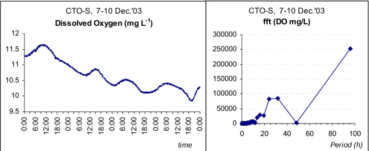
(18) common to almost all models or could be derived from the models themselves, namely initial slope or photosynthetic efficiency ( ), optimal light intensity or the light level that maximizes photosynthesis under given nutrient and temperature conditions (Eopt) as well as the maximal production rate or photosynthetic capacity (Pmax). Parameter. may be. obtained by calculating the limit of the derivative of P in relation to E as E approaches zero. In inhibition models, Eopt may be determined by calculating the light intensity that maximizes the same derivative (Duarte, in press). During the fitting procedure described above, Pmax, Eopt and. were estimated.. The first part of this section will deal with time-series analysis of the 5-d datasets for each survey. Further, some comparisons were made among data from different seasons, as well as between surface and bottom data along the year but only at station CTO, due to the above mentioned lack of a second updated multiprobe logger. The second part will deal with the analysis of the shorter datasets.. December 2003 survey – surface Temperature showed a regular temporal pattern, increasing during the morning towards a maximum at the early afternoon (Fig.3). Although dissolved oxygen (DO) patterns (.3) were similar to those of temperature, no significant correlation was found between them (maximum raw correlation coefficient (r.c.c.) was 0.48, for a time lag of almost 4h). DO saturation was generally below 90%, but always higher than 88% (Error! Reference source not found..3). DO maximum occurred in the morning and showed no significant correlation with pH (maximum r.c.c. = 0.46 for a 18h lag) (Error! Reference source not found..3). The DO morning maximum and the absence of correlation with pH, combined with a saturation level under 100%, suggests that photosynthesis was not compensating for net respiratory metabolism and that the ecosystem was predominantly heterotrophic. Figure WP1.3. Temperature variation (left) and fast Fourier transform power spectrum (right) at station B surface level, for a 96h sampling period on December 2003.. CTO-S, 7-10 Dec.'03 Temperature (ºC). 10.75. CTO-S, 7-10 Dec.'03 fft (T) 8000. 10.65 10.55. 6000. 10.45. 4000. 10.35. 2000. time. 18:00. 6:00. 12:00. 0:00. 18:00. 6:00. 12:00. 0:00. 18:00. 6:00. 12:00. 0:00. 18:00. 6:00. 12:00. 0:00. 10.25. 15. 0 0. 20. 40. 60. 80. 100. Period (h).

(19) CTO-S, 7-10 Dec.'03 fft (DO mg/L). CTO-S, 7-10 Dec.'03 Dissolved Oxygen (mg L-1). 100000. 9.5. 50000. 0:00. 10 12:00 18:00. 150000. 0:00 6:00. 10.5. 12:00 18:00. 200000. 18:00 0:00 6:00. 11. 6:00 12:00. 250000. 18:00 0:00. 11.5. 6:00 12:00. 300000. 0:00. 12. 0 0. 20. 40. 60. 80. 100. Period (h). time. Figure WP2.3. Dissolved oxygen variation (left) and fast Fourier transform power spectrum (right) at station B surface level, for a 96h sampling period on December 2003. CTO-S, 7-10 Dec.'03 Oxygen Saturation (%). 110. CTO-S, 7-10 Dec.'03 fft (DO sat) 2.50E+07. 105. 2.00E+07. 100. 1.50E+07. 95. 1.00E+07. 90. 5.00E+06 0:00. 18:00. 6:00 12:00. 0:00. 18:00. 6:00 12:00. 0:00. 6:00. 12:00 18:00. 0:00. 12:00 18:00. 6:00. 0:00. 85. 0.00E+00 0. 20. 40. 60. 80. 100. Period (h). time. Figure 3.3. Oxygen saturation variation (left) and fast Fourier transform power spectrum (right) at station B surface level, for a 96h sampling period on December 2003.. CTO-S, 7-10 Dec.'03 fft (pH). CTO-S, 7-10 Dec.'03 pH. 7.8 7.75. 3500. 7.7. 3000. 7.65. 2500 2000. 7.6. 1500. time. 0:00. 18:00. 6:00 12:00. 0:00. 18:00. 12:00. 0:00 6:00. 18:00. 6:00. 12:00. 0:00. 500. 12:00 18:00. 7.5 6:00. 1000. 0:00. 7.55. 0 0. 20. 40. 60. 80 100 Period (h). 16.

(20) Figure 4.3.pH variation (left) and fast Fourier transform power spectrum (right) at station B surface level, for a 96h sampling period on December 2003.. February 2004 survey – surface. In February, circadian patterns were easily detectable by Fourier analysis, for oxygen and pH (Figs. WP7.3, 8.3 and 9.3). Dissolved oxygen and pH were highly correlated (r.c.c.= 0.73) for a 4 min lag, although the highest correlation among all parameters was between pH and conductivity (r.c.c. = 0.87 for a 2 min lag). The high correlation between pH and dissolved oxygen was consistent with the underwater photosynthetic process, where oxygen was the end product of a chemical pathway that comprised CO2 consumption and a corresponding pH increase. The opposite was true during the night period, when community respiration leads to a pH reduction. Oxygen saturation was always above 100% (Error! Reference source not found..3), as a result of a net predomination of photosynthetic activity over heterotrophic metabolism. CTO-S, 16-19 Feb.'04 fft (T). CTO-S, 16-19 Feb.'04 Tem perature (ºC) 9.3. 2000. 9.2. 1500. 9.1. 1000. 9. 500. 8.9 0 0 10 20 30 40 50 60 70 80 90 10 0. 0:00. 16:00. 8:00. 0:00. 16:00. 8:00. 0:00. 16:00. 8:00. 0:00. 16:00. 8:00. 0:00. 8.8. Period (h). time. Figure WP5.3. Temperature variation (left) and fast Fourier transform power spectrum (right) at station B surface level, for a 96 h sampling period on February 2004.. CTO-S, 16-19 Feb.'04 fft (DO m g/L). CTO-S, 16-19 Feb.'04 -1. Dissolved Oxygen mg L ) 13.2. 3000. 13. 2500. 12.8. 2000. 12.6 12.4. 1500. 12.2. 1000. 12. 500. time. 0:00. 16:00. 8:00. 0:00. 16:00. 8:00. 0:00. 16:00. 8:00. 0:00. 16:00. 8:00. 0:00. 11.8. 0 0. 10. 20 30 40. 50 60 70 80. 90 100. Period (h). 17.

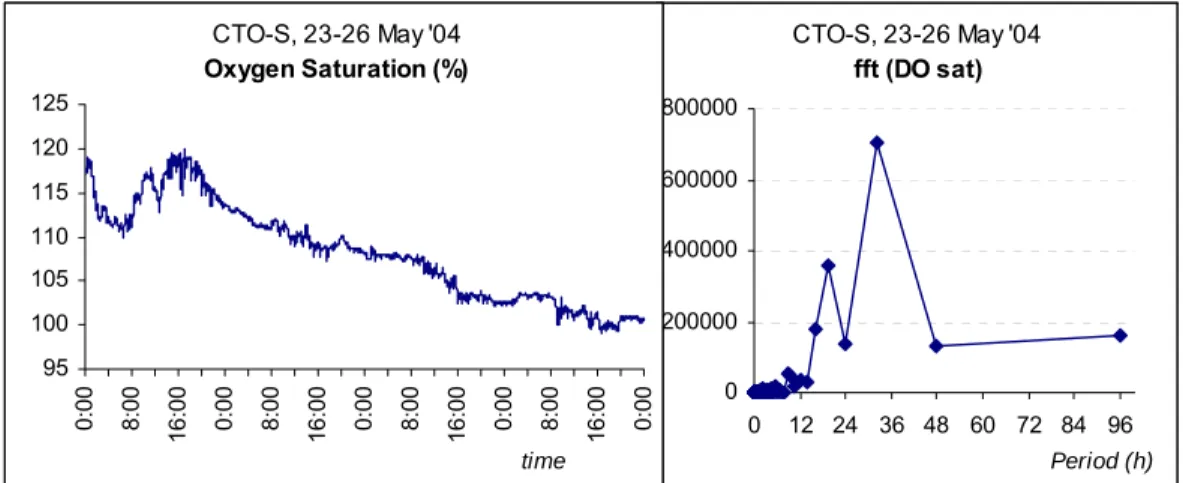
(21) Figure WP6.3. Dissolved oxygen variation (left) and fast Fourier transform power spectrum (right) at station B surface level, for a 96h sampling period on February 2004. CTO-S, 16-19 Feb.'04 fft (DO sat). CTO-S, 16-19 Feb.'04 Oxygen Saturation (%) 114. 200000. 112 150000. 110 108. 100000. 106 50000. 104. 0. 0:00. 16:00. 8:00. 0:00. 16:00. 8:00. 0:00. 8:00. 16:00. 0:00. 16:00. 8:00. 0:00. 102. 0. 10 20 30 40 50 60 70 80 90 100. Period (h). time. Figure WP7.3. Oxygen saturation variation (left) and fast Fourier transform power spectrum (right) at station B surface level, for a 96h sampling period on February 2004.. CTO-S, 16-19 Feb.'04 fft (pH). CTO-S, 16-19 Feb.'04 pH 8.05 8 7.95 7.9. time. 0:00. 16:00. 8:00. 0:00. 16:00. 8:00. 0:00. 16:00. 8:00. 0:00. 16:00. 8:00. 0:00. 7.85. 180 160 140 120 100 80 60 40 20 0 0. 12. 24. 36. 48. 60. 72 84 96 Period (h). Figure 8.3. pH variation (left) and fast Fourier transform power spectrum (right) at station B surface level, for a 96h sampling period on February 2004.. May 2004 survey – surface All variables showed considerable temporal variations, becoming quite difficult to visually identify cyclic events, contrasting with Fourier transform results where several periods were determined for each variable. It was possible to distinguish a 24h period only for temperature (Error! Reference source not found..3). In general, temperature reached a maximum value in the morning (~9h) that was followed by a strong rapid decline, after 18.

(22) which a smooth decrease was observed until the first hours of the day. These patterns probably depended on water inputs at different temperatures from upstream. A high r.c.c. (0.91) was found between DO concentration (Fig.3) and pH (Figure WP13.3) and for a zero min lag, corroborating the close chemical relationship between those variables. Oxygen saturation was always above 100% suggesting autotrophy dominance (Fig.3). As for previous datasets, cyclic events in chlorophyll concentration variations were only detected by Fourier transform and were not identified in the time series, even after data interpolation.. CTO-S, 23-26 May '04 fft (T). CTO-S, 23-26 May '04 Temperature (ºC) 18.5. 25000. 18. 20000 15000. 17.5. 10000. 17. 5000. 0:00. 16:00. 8:00. 0:00. 16:00. 8:00. 0:00. 16:00. 8:00. 0:00. 8:00. 16:00. 0:00. 16.5 0 0. 12 24 36 48 60 72 84 96. time. period (h). Figure WP9.3. Temperature variation (left) and fast Fourier transform power spectrum (right) at station B surface level, for a 96h sampling period on May 2004.. CTO-S, 23-26 May '04 fft (DO mg/L). CTO-S, 23-26 May '04 Dissolved Oxygen (mg/L). time. 0:00. 16:00. 8:00. 0:00. 0 16:00. 500. 9 8:00. 9.5 0:00. 1000. 16:00. 1500. 10. 8:00. 2000. 10.5. 0:00. 2500. 11. 16:00. 11.5. 8:00. 3000. 0:00. 12. 0. 12 24 36 48 60 72 84 96 Period (h). Figure WP10.3. Dissolved oxygen variation (left) and fast Fourier transform power spectrum (right) at station B surface level, for a 96h sampling period on May 2004.. 19.

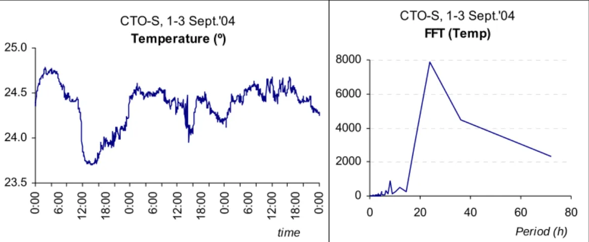
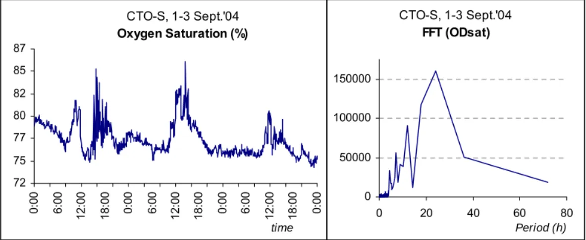
(23) CTO-S, 23-26 May '04 Oxygen Saturation (%). CTO-S, 23-26 May '04 fft (DO sat). 125. 800000. 120 600000. 115 110. 400000. 105 200000. 100. 0. 0:00. 16:00. 8:00. 0:00. 16:00. 8:00. 0:00. 16:00. 8:00. 0:00. 16:00. 8:00. 0:00. 95. 0. 12 24 36 48 60 72 84 96 Period (h). time. Figure WP11.3. Oxygen saturation variation (left) and fast Fourier transform power spectrum (right) at station B surface level, for a 96 h sampling period on May 2004.. CTO-S, 23-26 May '04 pH. CTO-S, 23-26 May '04 fft (pH) 300. 8.45. 250 200. 8.35. 150 8.25. 100 50 0:00. 8:00. 16:00. 0:00. 16:00. 8:00. 0:00. 16:00. 8:00. 0:00. 16:00. 8:00. 0:00. 8.15. 0 0. time. 12 24 36 48 60 72 84 96 Period (h). Figure WP12.3. pH variation (left) and fast Fourier transform power spectrum (right) at station B surface level, for a 96h sampling period on May 2004.. September 2004 survey – surface Circadian patterns were detectable by Fourier analysis for oxygen and pH (Figs. WP15.3, 16.3, and 17.3). Cross-correlation results revealed low r.c.c. among all variables (below 0.57). Despite the distinct periods determined by Fourier transform for DO and pH, their temporal variation were rather consistent with the expected relationships between those variables. In contrast with preceding two surveys, DO saturation was always below 100% (Figure WP16.3) suggesting heterotrophic dominance.. 20.

(24) CTO-S, 1-3 Sept.'04 FFT (Temp). CTO-S, 1-3 Sept.'04 Temperature (º). 25.0. 8000. 24.5. 6000 4000. 24.0. 2000 0:00. 18:00. 12:00. 6:00. 0:00. 18:00. 12:00. 6:00. 0:00. 18:00. 6:00. 12:00. 0:00. 23.5. 0 0. 20. 40. 60. 80. Period (h). time. Figure WP13.3. Temperature variation (left) and fast Fourier transform power spectrum (right) at station B surface level, for a 96 h sampling period on September 2004.. CTO-S, 1-3 Sept.'04 FFT (ODconc). CTO-S, 1-3 Sept.'04 Dissolved Oxygen (mg/L) 7.2. 2000. 7. 1500. 6.8 6.6. 1000. 6.4 6.2. 500. time. 0:00. 18:00. 6:00. 12:00. 0:00. 18:00. 12:00. 6:00. 0:00. 18:00. 12:00. 6:00. 0:00. 6. 0 0. 20. 40. 60 80 Period (h). Figure WP14.3. Dissolved oxygen variation (left) and fast Fourier transform power spectrum (right) at station B surface level, for a 96 h sampling period on September 2004.. 21.

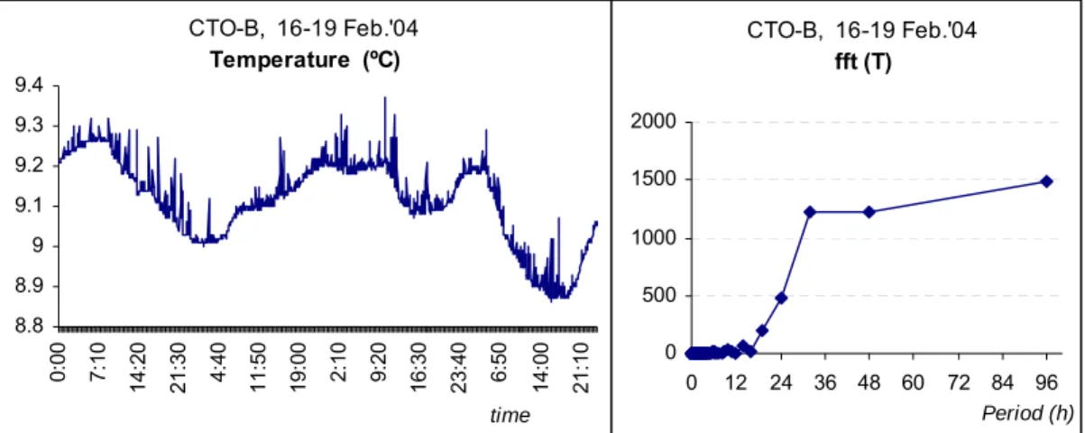
(25) CTO-S, 1-3 Sept.'04 FFT (ODsat). CTO-S, 1-3 Sept.'04 Oxygen Saturation (%) 87 85. 150000. 82 80. 100000. 77 50000. 75. 0. 0:00. 18:00. 12:00. 6:00. 0:00. 18:00. 12:00. 6:00. 0:00. 18:00. 12:00. 6:00. 0:00. 72 0. 20. 40. 60 80 Period (h). time. Figure WP15.3. Oxygen saturation variation (left) and fast Fourier transform power spectrum (right) at station B surface level, for a 96 h sampling period on September 2004. .. CTO-S, 1-3 Sept.'04 FFT (pH). CTO-S, 1-3 Sept.'04 pH. 7.65. 40 7.6 30 7.55 20 7.5 10. time. 0:00. 18:00. 12:00. 6:00. 0:00. 18:00. 12:00. 6:00. 0:00. 18:00. 12:00. 6:00. 0:00. 7.45 0 0. 20. 40. 60 80 Period (h). Figure WP16.3. pH variation (left) and fast Fourier transform power spectrum (right) at station B surface level, for a 96h sampling period on September 2004.. February 2004 survey – bottom (9 m) DO (Figure WP19.3) and pH (Fig.3) showed the expected direct relationship, varying instantaneously in a direct way readily evident from graphical interpretation. Highest correlation was observed for a one minute time lag (r.c.c.=0.67). Oxygen saturation was always above 100% (Error! Reference source not found..3), denoting a net autotrophic 22.

(26) metabolism of the system although measurements were carried out well below the light penetration zone (1% light saturation, or ~ 6 m). Oxygen was the only parameter with a well-defined variation pattern along the sampling period, where circadian cycles were easily identified.. CTO-B, 16-19 Feb.'04 Temperature (ºC). CTO-B, 16-19 Feb.'04 fft (T). 9.4. 2000. 9.3 9.2. 1500. 9.1 9. 1000. 8.9. 500 0. 21:10. 14:00. 6:50. 23:40. 16:30. 9:20. 2:10. 19:00. 11:50. 4:40. 21:30. 14:20. 7:10. 0:00. 8.8. 0. 12. time. 24 36 48 60. 72 84 96 Period (h). Figure WP17.3. Temperature variation (left) and fast Fourier transform power spectrum (right) at station B bottom level, for a 96h sampling period on February 2004.. CTO-B, 16-19 Feb.'04 fft (DO mg/L). CTO-B, 16-19 Feb.'04 Dissolved Oxygen (mgL-1) 13.4 13.2. 2000. 13. 1500. 12.8 12.6. 1000. 12.4. 500 0:00. 18:00. 12:00. 6:00. 0:00. 18:00. 12:00. 6:00. 0:00. 18:00. 6:00. 12:00. 0:00. 18:00. 12:00. 6:00. 0:00. 12.2. 0 0. 12 24 36 48 60 72 84 96 Period (h). time. Figure WP18.3. Dissolved oxygen variation (left) and fast Fourier transform power spectrum (right) at station B bottom level, for a 96 h sampling period on February 2004.. CTO-B, 16-19 Feb.'04 Oxygen Saturation (%). CTO-B, 16-19 Feb.'04 fft (DO sat). 116 160000. 114 112. 120000. 110. 80000. 108. 40000. 23. time. 0:00. 18:00. 12:00. 6:00. 0:00. 18:00. 12:00. 6:00. 0:00. 18:00. 6:00. 12:00. 0:00. 18:00. 12:00. 6:00. 0:00. 106 0 0. 12 24 36 48 60 72 84 96 Period (h).

(27) Figure WP19.3. Oxygen saturation variation (left) and fast Fourier transform power spectrum (right) at station B bottom level, for a 96 h sampling period on February 2004.. CTO-B, 16-19 Feb.'04 pH. CTO-B, 16-19 Feb.'04 fft (pH). 7.4 400. 7.3 7.2. 300. 7.1. 200. 7. 100. 0:00. 6:00. 12:00 18:00. 18:00 0:00. 6:00 12:00. 0:00. 12:00 18:00. 0:00 6:00. 18:00. 6:00 12:00. 0:00. 6.9 0 0. 12 24. 36 48. 60 72. time. 84 96 Period (h). Figure WP 20.3. pH variation (left) and fast Fourier transform power spectrum (right) at station B bottom level, for a 96 h sampling period on February 2004.. May 2004 survey – bottom. DO concentration increased during the first hours of the day, but the daily DO maximum occurred at different times of the day. Consequently, it was very difficult to identify a regular pattern of variation (.3). Nevertheless, the pattern followed the temperature trend (Error! Reference source not found..3). Fourier transform highlighted 32h and 48h periods, but were absent in temporal plots. Oxygen saturation was always above 100%, suggesting a net autotrophic metabolism (Figure WP23.3). In contrast with previous results, pH did not reveal any clear relationship with dissolved oxygen. In fact, the lowest r.c.c. found between them (0.45, for a 9 min lag) suggested the interference of external factors.. CTO-B, 23-26 May '04 fft (T). CTO-B, 23-26 May '04 Temperature (ºC) 17.9. 12000 10000. 17.4. 8000 6000. 16.9. 4000 2000. time. 0:00. 16:00. 8:00. 0:00. 16:00. 8:00. 0:00. 16:00. 8:00. 0:00. 16:00. 8:00. 0:00. 16.4. 0 0. 12 24 36 48 60 72 84 96 period (h). 24.

(28) Figure WP21.3. Temperature variation (left) and fast Fourier transform power spectrum (right) at station B bottom level, for a 96h sampling period on May 2004.. CTO-B, 23-26 May '04 fft (DO mg/L). CTO-B, 23-26 May '04 Dissolved Oxygen (mg/L) 11. 5000 4000. 10.5 3000 2000. 10. 1000 0. 19:40. 11:20. 3:00. 18:40. 10:20. 2:00. 17:40. 9:20. 1:00. 16:40. 8:20. 0:00. 9.5. 0. 12 24 36 48 60 72 84 96 period (h). time. Figure WP22.3. Dissolved oxygen variation (left) and fast Fourier transform power spectrum (right) at station B bottom level, for a 96 h sampling period on May 2004.. CTO-B, 23-26 May '04 Oxygen Saturation (%). CTO-B, 23-26 May '04 fft (DO sat). 115. 1000000. 110. 800000 600000. 105. 400000. 100. 200000. 0:00. 16:00. 8:00. 0:00. 16:00. 8:00. 0:00. 16:00. 8:00. 0:00. 16:00. 8:00. 0:00. 95. 0 0. 12 24 36 48 60 72 84 96. time. period (h). Figure WP23.3. Oxygen saturation variation (left) and fast Fourier transform power spectrum (right) at station B bottom level, for a 96 h sampling period on May 2004.. CTO-B, 23-26 May '04 fft (pH). CTO-B, 23-26 May '04 pH 1000. 7.8. 800. 7.6. 600. 7.4. 400. 7.2. 200. time. 0:00. 16:00. 8:00. 0:00. 16:00. 8:00. 0:00. 16:00. 8:00. 0:00. 16:00. 8:00. 0:00. 7. 0 0. 12 24 36 48 60 72 84 96 period (h). 25.

(29) Figure WP24.3. pH variation (left) and fast Fourier transform power spectrum (right) at station B bottom level, for a 96 h sampling period on May 2004.. 26.

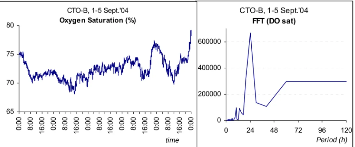
(30) September 2004 survey – bottom A 24h period was identified by Fourier transform for temperature (Error! Reference source not found..3), oxygen concentration (Fig.3) and oxygen saturation (Figure WP27.3). Temperature was relatively high (always above 23.5ºC) as expected for this time of the year with minimum values consistently observed during the night. Oxygen saturation was always below 100%, indicating that respiratory metabolism prevailed over photosynthesis. On the other hand, Fourier transform of pH data revealed events with 20h and 30h periods, which were not visually identified in the time series data (Error! Reference source not found..3). Moreover, the expected relationship between this variable and oxygen was not apparent.. CTO-B, 1-5 Sept.'04 FFT (Temp). CTO-B, 1-5 Sept.'04 Temperature (ºC). 24.9. 16000. 24.7 24.5. 12000. 24.3 24.1. 8000. 23.9. 4000. 23.7 0:00. 8:00. 16:00. 0:00. 8:00. 16:00. 0:00. 8:00. 16:00. 0:00. 8:00. 16:00. 0:00. 16:00. 8:00. 0:00. 23.5. 0 0. 24. 48. 72. time. 96 120 Period (h). Figure WP25.3. Temperature variation (left) and fast Fourier transform power spectrum (right) at station B bottom level, for a 96h sampling period on September 2004.. CTO-F, 1-5 Sept.'04 Dissolved Oxygen (mg/L). 6.7. CTO-B, 1-5 Sept.'04 FFT (DO conc). 6.5. 4000. 6.3. 3000. 6.1. 2000. 5.9. 1000. time. 0:00. 16:00. 8:00. 0:00. 16:00. 8:00. 0:00. 16:00. 8:00. 0:00. 16:00. 8:00. 0:00. 16:00. 8:00. 0:00. 5.7. 0 0. 24. 48. 72. 96. 120. Period (h). Figure WP26.3. Dissolved oxygen variation (left) and fast Fourier transform power spectrum (right) at station B bottom level, for a 96h sampling period on September 2004.. 27.

(31) CTO-B, 1-5 Sept.'04 FFT (DO sat). CTO-B, 1-5 Sept.'04 Oxygen Saturation (%). 80. 600000 75. 400000 70. 200000. 0. 0:00. 8:00. 16:00. 0:00. 8:00. 16:00. 0:00. 8:00. 16:00. 0:00. 8:00. 16:00. 0:00. 8:00. 16:00. 0:00. 65. 0. 24. 48. 72. time. 96 120 Period (h). Figure WP27.3. Oxygen saturation variation (left) and fast Fourier transform power spectrum (right) at station B bottom level, for a 96h sampling period on September 2004.. CTO-B, 1-5 Sept.'04 FFT (pH). CTO-B, 1-5 Sept.'04 pH. 7.8. 600. 7.7 7.6. 400. 7.5. 200. time. 0:00. 16:00. 8:00. 0:00. 8:00. 16:00. 0:00. 16:00. 8:00. 0:00. 16:00. 8:00. 0:00. 16:00. 8:00. 0:00. 7.4. 0 0. 24. 48. 72. 96 120 Period (h). Figure WP28.3. pH variation (left) and fast Fourier transform power spectrum (right) at station B bottom level, for a 96h sampling period on September 2004.. Seasonal Analysis The seasonal analysis was performed with the 96h datasets and was restricted to the upstream station CTO since at this station a complete surface-bottom data set was obtained throughout the study. At ETA station, the lack of a new multiprobe (never 28.

(32) purchased following the recommendations of the evaluation panel, and the malfunctioning of an existing old equipment (limited to temperature and conductivity) restricted the continuous gathering of data to the surface. CTO-S Tem perature (ºC). CTO-S Dissolved Oxygen (m g/L) 14. 30. 12. 25. 10. 20. 8. 15. 6. 10. 4. 5. 2. 0. 0 7-10 Dec. 15-20 Feb 23-26 May. 1-3 Sept. CTO-S Oxygen Saturation (%). 7-10 Dec. 1-3 Sept. CTO-S pH. 8.5. 120. 15-20 Feb 23-26 May. 100 8. 80 60. 7.5. 40 20 0. 7 7-10 Dec. 15-20 Feb 23-26 May. 1-3 Sept. 7-10 Dec. 15-20 Feb 23-26 May. 1-3 Sept. Figure WP29.3. Comparison among mean values of environmental variables, measured at sampling station B surface level (CTO-S), along the year.. Surface (Figure WP29.3) Temperature and oxygen showed an inverse pattern of variation along the year. As temperature rose, dissolved oxygen decreased as well as oxygen saturation. Mean oxygen saturation was below 100% only in September. pH showed an identical seasonal pattern, increasing from February until May and then decreasing in September. Bottom (Figure WP30.3) Temperature increased from February to September as dissolved oxygen decreased to half values in the same period. An increase in pH was also observed along the year, but it was very slight (variation amplitude of only 0.3). 29.

(33) CTO-B Dissolved Oxygen (m g/L). CTO-B Tem perature (ºC). 14. 30. 12. 25. 10. 20. 8. 15. 6. 10. 4. 5. 2. 0. 0 16-19 Feb. 23-26 May. 1-6 Sept. CTO-B Oxygen Saturation (%). 16-19 Feb. 1-6 Sept. CTO-B pH. 7.7. 120. 23-26 May. 7.6. 100. 7.5. 80. 7.4. 60. 7.3 7.2. 40. 7.1. 20. 7. 0. 6.9 16-19 Feb. 23-26 May. 1-6 Sept. 16-19 Feb. 23-26 May. 1-6 Sept. Figure WP30.3. Comparison among mean values of environmental variables, measured at sampling station B bottom level (CTO-B), along the year. Overall comparison between surface and bottom data The comparison between surface and bottom environment was only possible for the year 2004 (February, May and September), using the 96-h data set. Bottom and surface mean values of dissolved oxygen and oxygen saturation decreased from winter till summer. An overall heterotrophic metabolism was apparent in the hottest season (September) at both depth levels.. Station ETA Mean values of all measured environmental variables were similar for surface and bottom data, except for dissolved oxygen, which was always higher at bottom (Figure WP 31.3). These higher levels of dissolved oxygen at lower depths suggest that heterotrophic metabolism was not consuming all the oxygen that was being produced at surface or the existence of DO transfers, either top-down or longitudinal.. 30.

(34) ETA SURFACE vs BOTTOM (24h) Dissolved Oxygen. ETA SURFACE vs BOTTOM (24h) Oxygen Saturation 160. 16 14. 140. 12 10. 120 100. 40. 8 6 4. 20. 2. 80 60. 0. 0 Dec. Feb. Surface. M ay1. Dec. M ay2. Feb Surface. Bottom. ETA SURFACE vs BOTTOM (24h) Tem perature. May1. May2. Bottom. ETA SURFACE vs BOTTOM (24h) pH. 45 40 35 30 25 20 15 10 5 0. 10 9 8 7 6 5 4 3 2 1 0 Dec. Feb. Surface. May1. Bottom. May2. Dec. Feb. May1. Surface. Bottom. May2. Figure WP31.3 Comparison between surface and bottom 24h data measured at ETA sampling station, for each season.. Station CTO At CTO station large differences were not detected between surface and bottom data along the year, except for pH, that was relatively higher at surface in February and May (Figure WP32.3). As mean temperature increased along the year, mean dissolved oxygen decreased and, in Septembe,r this value was half of the February value. Mean oxygen saturation variation along the year was less pronounced and only in May it was below 100%.. 31.

(35) CTO SURFACE vs BOTTOM Oxygen Saturation. CTO SURFACE vs BOTTOM Dissolved Oxygen 14. 120. 12. 100. 10. 80. 8. 60. 6. 40. 4. 20. 2 0. 0 Feb. May. Surface. Sept. Feb. May. Surface. Bottom. CTO SURFACE vs BOTTOM Tem perature. Sept. Bottom. CTO SURFACE vs BOTTOM pH 8.5. 30 25. 8. 20. 7.5. 15 10. 7. 5. 6.5. 0 Feb. May. Surface. Sept. Bottom. Feb. May Surface. Sept Bottom. Figure WP32.3. Comparison between surface and bottom 96h data measured at CTO sampling station, for each season. Analysis of 25-h datasets DO, temperature and pH ranges observed at both stations over the sampling period are synthesized in Tables WP1.3-WP4.3. Diurnal variability of chlorophyll, nutrient concentrations and river flow are summarized in Figs. WP33.3 through WP40.3. Correlation analysis did not reveal any clear influence of river flow on the remaining variables at short (25-h) time scales. The obtained results suggest that river flow may be strongly influence the behaviour of some variables in specific occasions, but without any consistent overall pattern. In fact, significant correlations (p < 0.05) between river flow and other variables were observed solely in three out of fifteen 25 h-datasets (station B X eight sampling occasion, plus station A X seven sampling occasions). However, these correlations were not consistent between the four mentioned datasets. For example, in two of them, photosynthetic pigments were significantly correlated with river flow, whereas in the third one only silicate exhibited a significant correlation with flow (p< 0.05). 32.

(36) Regarding long (seasonal) time scales, a significant negative correlation (p < 0.05) was observed between river flow and photosynthetic pigments. This may be explained by the fact that chlorophyll concentrations reached highest values in May, whereas river flow attained maximums in December and February i.e. during the coldest and the less light availability period of the year. Cluster analysis suggested a positive relationship between river flow and phosphate concentrations at seasonal time scales. Table WP1.3. Range values measured for dissolved oxygen saturation (DOsat) and concentration (DOconc), temperature (T) and pH for sampling station A (ETA) at surface level. ETA surface DO sat (%) DO conc (mg/L) T (ºC) pH. December. February. May. September. 86.1 – 108.1. 95.7 – 101.8. 92.3 – 108.7. ----------------. 4.52 – 16.54. 13.47 – 15.04. 9.48 – 11.43. ----------------. 10.31 – 10.81 6.93 – 7.26. 8.89 – 9.18 7.12 – 7.55. 16.91 – 18.13 7.39 – 8.26. -------------------------------. Table WP2.3. Range values measured for dissolved oxygen saturation (DOsat) and concentration (DOconc), temperature (T) and pH for sampling station A (ETA)at bottom level. ETA bottom DO sat (%) DO conc (mg/L) T (ºC) pH. December. February. May. September. 83.8 – 148.1. 117.2 – 130.6. 98.6 – 119.3. ----------------. 4.52 – 16.54. 13.47 – 15.04. 9.48 – 11.43. ----------------. 10.34 -51.3 7.1 – 8.04. 8.9 – 9.2 6.76 – 7.4. 16.87 – 17.52 7.02 – 9.78. -------------------------------. Table WP3.3. Range values measured for dissolved oxygen saturation (DOsat) and concentration (DOconc), temperature (T) and pH for sampling station B (CTO) at surface level. CTO surface DO sat (%) DO conc (mg/L) T (ºC) pH. December. February. May. September. 87.9 – 104.9. 104.9 - 113. 99.1 – 119.9. 73.7 – 85.6. 9.83 -11.67. 12.07 – 13.1. 9.52 – 11.38. 6.17 – 7.16. 10.24 – 10.66 7.52 – 7.72. 8.83 – 9.25 7.91 – 8.01. 16.93 -18.27 8.18 – 8.48. 23.7 -24.78 7.46 – 7.6. 33.

(37) Table WP4.3. Range values measured for dissolved oxygen saturation (DOsat) and concentration (DOconc), temperature (T) and pH for sampling station B (CTO) at bottom level. CTO bottom DO sat (%) DO conc (mg/L) T (ºC) pH. December. February. May. September. ----------------. 108.2 – 115.1. 103.2 – 112.8. 68.1 – 79.2. ----------------. 12.43 – 13.34. 9.96 – 10.84. 5.76 – 6.67. -------------------------------. 8.86 – 9.37 7.05 – 7.31. 16.7 – 17.8 7.31 – 7.76. 23.62 – 24.66 7.46 – 7.76. 34.

(38) CTO, 7-8 Dec.'03 CHLa. ETA, 7-8 Dec.'03 CHLa. 2.7. 2.5 2.5. 2.3. μ. μ. 2.3. 2.1 2.1. 1.9 1.9. 1.7 1.7. 1.5 8h. 11h. 14h. 17h. 20h 23h. 2h. 5h. 1.5. 8h. 8h. time. 11h. 14h. 17h. 20h. 23h. 2h. 5h. 8h. time. ETA, 7-8 Dec.'03 Nutrients. CTO, 7-8 Dec.'03 Nutrients 3. 4. 140. 130. 120. 125. 3. 100. 2. 120. 80. 2. 60 1. 115. 40. 1. 110. 20 0. 0. 0 8h. 11h. 14h 17h 20h 23h 2h. NO2-. NH4. 5h. 105 8h. 8h. P O4. NO3-. 11h. 14h 17h 20h 23h 2h. NO2-. NH4. 5h. 8h. P O4. NO3-. 7-8 Dec. '03 3. 2750. Flow (m /s). 2250 1750 1250 750. 9:00. 8:00. 7:00. 6:00. 5:00. 4:00. 3:00. 2:00. 1:00. 0:00. 23:00. 22:00. 21:00. 20:00. 19:00. 18:00. 17:00. 16:00. 15:00. 14:00. 13:00. 12:00. 11:00. 10:00. 9:00. 8:00. 7:00. 250. time. Figure WP33.3. Chlorophyll-a and nutrients data measured at both sampling stations (upper charts), corresponding to a 24h sampling period from 7 to 8 of December 2003. Bottom chart represents the flow regime and the dots the moments when chlorophyll-a and nutrients were sampled. 35.

(39) CTO, 10-11 Dec.'03 CHLa. 4. 3.5 3.0 CHLa ( g/L). CHLa ( g/L). 3.5 3 2.5 2. 8h 11h 14h 17h 20h 23h 2h. 2.0. 8h 11h 14h 17h 20h 23h 2h. 5h 8h time. CTO, 10-11 Dec.'03 Nutrients. 5. 140. 4. 135. 3. 5h 8h time. ETA, 10-11 Dec.'03 Nutrients. 145 140 135. (μ. 4 (μ. 2.5. 1.5. 1.5. 3 130. 130. 2. μ. μ. 2. 125 125. 1. 1 120. 0. 120 8h. 11h. NO2-. 1350. ETA 10-11 Dec.'03 CHLa. 14h 17h 20h 23h 2h NH4. 5h. P O4. 0. 115 8h. 8h NO3-. 11h. NO2-. 14h 17h 20h 23h NH4. 2h. 5h. 8h. P O4. NO3-. 10-11 Dec. '03 3 Flow (m /s). 1300 1250 1200 1150 1100 time. Figure WP34.3. Chlorophyll-a and nutrients data measured at both sampling stations (upper charts), corresponding to a 24h sampling period from 10 to 11 of December 2003. Bottom chart represents the flow regime and the dots the moments when chlorophyll-a and nutrients were sampled.. 36.

(40) CTO, 15-16 Feb.'04 CHLa. 3.5. 2.6 2.5 CHLa ( g/L). 3.0 CHLa ( g/L). ETA, 15-16 Feb.'04 CHLa. 2.5 2.0. 2.4 2.3 2.2. 1.5. 2.1. 1.0. 2.0. 7h 10h 13h 16h 19h 22h 1h. 4h 7h time. 7h 10h 13h 16h 19h 22h 1h. ETA, 15-16 Feb.'04 Nutrients. CTO, 15-16 Feb.'04 Nutrients 3. 5. 80. 80. 4. 60 2. 60. 3 40. 40 μ. 2. 1 20. 0 10h 13h. NO2-. 16h. 19h 22h. NH4. 1h. 4h. 0. 0 7h. 7h. P O4. 20. 1. 0 7h. 10h. 13h. NO2-. NO3-. 16h. 19h 22h. NH4. 1h. 4h. 7h. P O4. NO3-. 15-16 Feb. '04 FLOW (m 3/s). 1000 900 800 700 600. 8:00. 7:00. 6:00. 5:00. 4:00. 3:00. 2:00. 1:00. 0:00. 23:00. 22:00. 21:00. 20:00. 19:00. 18:00. 17:00. 16:00. 15:00. 14:00. 13:00. 12:00. 11:00. 9:00. 10:00. 8:00. 7:00. 500 6:00. (μ. 4h 7h time. time. Figure WP35.3. Chlorophyll-a and nutrients data measured at both sampling stations (upper charts), corresponding to a 24h sampling period from 15 to 16 of February 2004. Bottom chart represents the flow regime and the dots the moments when chlorophyll-a and nutrients were sampled.. 37.

(41) ETA 18 Feb.'04 CHLa. CTO, 18-19 Feb.'04 CHLa 3.4. 2.8 CHLa ( g/L). 3.2 CHLa ( g/L). 2.6 2.4. 3.0 2.8 2.6 2.4. 2.2. 2.2 2.0. 2.0 7h 10h 13h 16h 19h 22h 1h. CTO, 18-19 Feb.'04 Nutrients. 3. 7h 10h 13h 16h 19h 22h 1h. 4h 7h time. 7h. time. ETA, 18 Feb.'04 Nutrients. 180. 2. 4h. 4. 100 80. 3. 160. 60 2. 1. 40. 140 1. 0. 120 7h. 10h 13h. NO2-. 16h 19h 22h NH4. 1h. 4h. 20. 0. 7h. 0 7h. P O4. NO3-. 10h. 13h 16h. NO2-. 19h 22h. NH4. 1h. 4h. 7h. P O4. NO3-. 18-19 Feb. '04 FLOW (m 3/s). 900 850 800 750 700. 8:00. 7:00. 6:00. 5:00. 4:00. 3:00. 2:00. 1:00. 0:00. 23:00. 22:00. 21:00. 20:00. 19:00. 18:00. 17:00. 16:00. 15:00. 14:00. 13:00. 12:00. 11:00. 9:00. 10:00. 8:00. 7:00. 6:00. 650. time. Figure WP36.3 Chlorophyll-a and nutrients data measured at both sampling stations (upper charts), corresponding to a 24h sampling period from 18 to 19 of February 2004. Bottom chart represents the flow regime and the dots the moments when chlorophyll-a and nutrients were sampled. 38.

(42) CTO, 23-24 May '04 CHLa. 11. 15 14. 10. 13 12. CHLa ( g/L). CHLa ( g/L). 16. ETA, 23-24 May '04 CHLa. 11 10 9 8. 9 8 7. 7. 6 7h 10h 13h 16h 19h 22h 1h. 4h. 7h 10h 13h 16h 19h 22h 1h. 7h. time. CTO, 23-24 May '04 Nutrients. 12. 200. ETA, 23-24 May '04 Nutrients. 12. 10. 4h 7h time. 200. 10 150. 150. 8. 8. 6. 100. 6. 100. \ 4. 4 50. 50. 2. 2. 0. 0 7h. 10h 13h 16h 19h 22h. NO2-. NH4. 1h. 4h. 0. 7h. 0 7h. P O4. NO3-. 10h. 13h 16h. NO2-. 19h 22h. NH4. 1h. 4h. 7h. P O4. NO3-. 23-24 May'04 FLOW (m3/s). 1200 1000 800 600 400 200 0. 8:00. 7:00. 6:00. 5:00. 4:00. 3:00. 2:00. 1:00. 0:00. 23:00. 22:00. 21:00. 20:00. 19:00. 18:00. 17:00. 16:00. 15:00. 14:00. 13:00. 12:00. 11:00. 9:00. 10:00. 8:00. 7:00. 6:00. -200. time. Figure 37.3. Chlorophyll-a and nutrients data measured at both sampling stations (upper charts), corresponding to a 24h sampling period from 23 to 24 of May 2004. Bottom chart represents the flow regime and the dots the moments when chlorophyll-a and nutrients were sampled. 39.

(43) 10. 14 13. 9. 12 11. CHLa ( g/L). CHLa ( g/L). CTO, 26-27 May '04 CHLa. 8. 10 9. 7. 8 7. 6. 6 5 7h 10h 13h 16h 19h 22h 1h. 5. 7h 10h 13h 16h 19h 22h 1h. 4h 7h time. CTO, 26-27 May '04 Nutrients. 4. ETA 26 May'04 CHLa. 4h 7h time. ETA, 26 May '04 Nutrients. 100. 4. 100. 75. 3. 75. 50. 2. 50. 25. 1. 25. 0. 0. 3 2 1 0 7h. 10h 13h 16h 19h 22h. NO2-. NH4. 1h. 4h. 0 7h. 7h. P O4. 10h. 13h. 16h. NO2-. NO3-. 19h 22h. NH4. 1h. 4h. 7h. P O4. NO3-. 26-27 Maio'04 FLOW (m3/s). 1000 800 600 400 200. 8:00. 7:00. 6:00. 5:00. 4:00. 3:00. 2:00. 1:00. 0:00. 23:00. 22:00. 21:00. 20:00. 19:00. 18:00. 17:00. 16:00. 15:00. 14:00. 13:00. 12:00. 11:00. 9:00. 10:00. 8:00. 7:00. 6:00. 0. time. Figure 38.3. Chlorophyll-a and nutrients data measured at both sampling stations (upper charts), corresponding to a 24h sampling period from 26 to 27 of May 2004. Bottom chart represents the flow regime and the dots the moments when chlorophyll-a and nutrients were sampled.. 40.

(44) CTO 1-2 Sept. '04 CHLa. 6.0. 7. 5.5. 6 CHLa ( g/L). CHLa ( g/L). ETA, 1-2 Sept. '04 CHLa. 5.0. 5 4. 4.5. 3. 4.0 7h 10h 13h 16h 19h 22h 1h. CTO, 1-2 Sept. '04 Nutrients. 6. 7h 10h 13h 16h 19h 22h 1h. 4h 7h time. 80. 4h 7h time. ETA, 1-2 Sept. '04 Nutrients. 4. 80. 5 4. 3. 60. 2. 40. 1. 20. 75. 3 2. 70. 1 0. 65 7h. 10h. 13h. 16h. NO2-. 19h. 22h. NH4. 1h. 4h. 0. 7h. 0 7h. P O4. 10h. 13h. 16h. NO2-. NO3-. 19h. 22h. NH4. 1h. 4h. 7h. P O4. NO3-. 1-2 Sept. '04 FLOW (m 3/s). 1000 800 600 400 200. 8.00. 7.00. 6.00. 5.00. 4.00. 3.00. 2.00. 1.00. 0.00. 23.00. 22.00. 21.00. 20.00. 19.00. 18.00. 17.00. 16.00. 15.00. 14.00. 13.00. 12.00. 11.00. 9.00. 10.00. 8.00. 7.00. 6.00. 0. time. Figure 39.3. Chlorophyll-a and nutrients data measured at both sampling stations (upper charts), corresponding to a 24h sampling period from 1 to 2 of September 2004. Bottom chart represents the flow regime and the dots the moments when chlorophyll-a and nutrients were sampled.. 41.

(45) CTO, 5-6 Sept. '04 CHLa. 7.5. 6.5 5.5 CHLa ( g/L). 6.5 CHLa ( g/L). ETA, 5-6 Sept. '04 CHLa. 5.5 4.5. 4.5 3.5. 3.5. 2.5 7h 10h 13h 16h 19h 22h 1h. 4h 7h time. CTO, 5-6 Sept. '04 Nutrients. 10 8. 7h 10h 13h 16h 19h 22h 1h. 4h 7h time. ETA, 5-6 Sept. '04 Nutrients. 80. 4. 60. 3. 60. 40. 2. 40. 20. 1. 20. 0. 0. 80. 6 4 2 0 7h. 10h. 13h. 16h. NO2-. 19h 22h. NH4. 1h. 4h. 7h. P O4. 0 7h. NO3-. 10h. 13h. 16h. NO2-. 19h 22h. NH4. 1h. 4h. 7h. P O4. NO3-. 5-6 Sept. '04 FLOW (m 3/s). 400 300 200 100. 8.00. 7.00. 6.00. 5.00. 4.00. 3.00. 2.00. 1.00. 0.00. 23.00. 22.00. 21.00. 20.00. 19.00. 18.00. 17.00. 16.00. 15.00. 14.00. 13.00. 12.00. 11.00. 9.00. 10.00. 8.00. 7.00. 6.00. 0. time. Figure 40.3. Chlorophyll-a and nutrients data measured at both sampling stations (upper charts), corresponding to a 24h sampling period from 5 to 6 of February 2004. Bottom chart represents the flow regime and the dots the moments when chlorophyll-a and nutrients were sampled.. 42.

(46) Table WP5.3 summarizes the results obtained by fitting Steels’ P/I equation (Steele, 1962) to production light data (cf. – Methodology – Data analysis). The analysis of these results suggests the following patterns: 1) Highest Pmax values were observed in May and September (up to five fold higher than in December and February); 2). was also generally higher in May and September. Therefore, phytoplankton was not only more productive but also more efficient in using available light;. 3). decreased from morning to dawn, suggesting that in early morning phytoplankton cells were more efficient in using light – presumably, dark adapted;. 43.

(47) Table WP5.3. Photosynthetic parameters Pmax (maximum photosynthetic rate), Iopt (optimal light intensity) and Slope (initial slope of the P-I relationship or quantum yield) estimated from the results of primary production measurements under various light intensities, conducted during the sampling campaigns. The second column indicates the incubation period in hours AM. The variance explained by all P-I curves obtained was significantly larger than the residual variance (p < 0.05), as tested by Analysis of Variance.. Hours Dec 7th 2003 Feb 15th 2004 Feb 19th 2004 May 22nd 2004 May 26th 2004 Sep 1st 2004 Sep 5th 2004. 8 – 10 12-12.33 12-15 15-17 8 – 10 11-13 12-13.25 8 – 10 11-13 14-16 7-8 10-11 13-14 16-17 7-8 10-11 13-14 16-17 7–8 12-13 16-17 7–8 12-13 16-17. Pmax. (mgC mg Chla-1 h-1). 0.93 1.25 0.89 0.57 0.88 1.16 1.19 0.86 1.44 1.01 2.01 3.23 2.58 1.97 2.01 3.69 4.30 5.33 5.00 5.83 3.44 2.86 3.34 1.61. Eopt.  mol quanta m-2 s-1). 191.3 238.2 404.8 347.5 268.4 492.5 425.2 219.6 426.0 579.5 436.6 994.0 999.4 1015.3 246.9 523.3 608.6 762.2 149.7 414.2 927.2 28.27 717.7 666.5. (mgC mg Chla-1 h-1 mol quanta m2 s1). 0.013 0.014 0.006 0.004 0.009 0.006 0.007 0.011 0.009 0.005 0.013 0.009 0.007 0.005 0.022 0.019 0.019 0.019 0.091 0.038 0.010 0.275 0.013 0.007. 44.

(48) WP4/WP5 – Implementation of a 2D vertically resolved model/ Model calibration and implementation. Introduction This section describes the implementation of WP4 coupled with WP5. The model was implemented and tested after concluding its calibration and validation based upon the data gathered during WP2 and WP3 (Figure WP1.4).. Figure WP1.4. Model flow chart.. Model conceptual and tools The main processes and variables simulated by the model are summarized in Table WP1.4. There are feedbacks between most processes and variables. For example, water temperature depends on heat exchanges between the river, the atmosphere and other. 45.

(49) water masses, but it also depends on the radiation budget. Phytoplankton production depends on light intensity, water temperature and nutrient concentrations. The concentration of any variable depends not only on its production and decay processes but also on transport (advection and diffusion) by river flow. Horizontal and vertical transport is calculated with a hydrodynamic 2D vertically resolved sub-model. This depends on river flow and horizontal pressure gradients due to differences in water level (barotropic pressure gradients) and density (baroclinic pressure gradients). The model was implemented in EcoDyn – a shell for ecological modelling in windows environment (Duarte & Pereira, in prep) - following an object oriented programming methodology. Initially, it has been planned to use EcoWin (Ferreira, 1995). However, several technical difficulties in using EcoWin for coupled physical-biogeochemical modelling justified the development and implementation of EcoDyn, by the CEMAS research team. In Figure WP2.4 the model interface is shown together with some graphical outputs. In EcoDyn, hydrodynamic transport, water temperature (Figure WP3.4), nutrients and phytoplankton are implemented though different sub-models, as classes (in object oriented programming language), written in C++ code. These classes may be plugged in or unplugged through the software interface (see the list box in Figure WP1.4. Each variable is described by a differential equation which is a mass balance including production, decay and transport processes (Table WP2.4). The variables are resolved simultaneously for each model compartment and layer and transported among them by the transport sub-model.. 46.

(50) Table WP1.4. Main processes and variables simulated by the model. There are feedbacks between most of the processes and variables as in the real system (see text).. Physical processes and variables Thermodynamic. Transport. Heat exchanges between the water and the Processes atmosphere and between different water masses Water temperature and density. Advection and diffusion of water. Nutrient Phytoplankton consumption and production and regeneration decay. Nitrogen and phosphorus concentrations. Phytoplankton biomass. Flow vs. Time 600 500 400. Flow. Variables. Current velocity and flow. Radiation balance Water reflection and emission and sun light absorption Light intensity as a function of depth and water turbidity. Biogeochemical processes and variables Nutrients Phytoplankton. 300 200 100 0 -100. 0. 50. 100. 150 Time (hours). 200. 250. 300. Figure WP2.4. Model interface of EcoDyn.. 47.

(51) Figure WP3.4. Temporal simulations of flow and temperature for a summer situation.. The detailed equations for the 2D transport, the nutrient and the phytoplankton sub-model rate processes (the parcels of equations depicted in Table WP2.4) are presented together with the respective parameters in Annexes I and II.. 48.

(52) Table WP2.4. Main model equations representing the changes in the state variables as a function of time. The equations are solved for all 22 model compartments and 7 layers. For details regarding current speed (transport model) refer to Annexes I and II. Note that the sinks for phytoplankton are sources for the dissolved nutrients and vice-versa. Fluxes are expressed in Carbon, Nitrogen and Phosphorus units (see text).. Current speed (m s-1). du = pressure _ gradient _ force ± advection _ of _ momentum dt ± diffusion _ of _ momentum ± drag _ forces Water temperature changes (ºC d-1). (WP4. 1). d T ij. = solar _ radiation + atmospheric _ emission − water _ emission (WP4. dt 2) −latent _ heat ± heat _ advection ± heat _ diffusion Dissolved mineral nitrogen variation (μmol L-1 d-1). d DIN ij. = PHYRespN ij + PHYExudN ij + PHYMortN ij + PHYSetN ij dt + DINLloads ij − PHYUptakeN ij ± Advection ± Diffusion. (WP4. 3). DINij = Nitrateij + Nitriteij + Ammoniumij Dissolved mineral phosphorus variation (μmol L-1 d-1). d P ij. = PHYRespP ij + PHYExudP ij + PHYMortP ij + PHYSetP ij dt + PLoads ij − PHYUptakeP ij ± Advection ± Diffusion. (WP4.4 ). Phytoplankton carbon biomass changes (μg C L-1 d-1). ⎛ PHYGPP ij − PHYExud ij − ⎞ ⎟ = PHYC ij ⎜ ⎜ PHYResp ij − PHYMort ij − PHYSet ij ⎟ dt ⎝ ⎠ ± Advection ± Diffusion d PHYC ij. This is also expressed as μg Chl L-1 h-1 (PHYChlij) using a Carbon:Chlorophyll ratio of 50 Jørgensen & Jørgensen (1991). (WP4. 5). Phytoplankton nitrogen biomass changes (μg N L-1 d-1). d PHYN ij. = PHYUptakeN ij − PHYRespN ij − PHYExudN ij dt − PHYMortN ij − PHYSetN ij ± Advection ± Diffusion. Phytoplankton phosphorus biomass changes (μg P L-1 d1) d PHYP ij = PHYUptakeP ij − PHYRespP ij − PHYExudP ij dt − PHYMortP ij − PHYSetP ij ± Advection ± Diffusion. (WP4. 6). (WP4. 7). 49.

(53) PHYGPPij PHYExudij PHYRespij PHYMortij PHYSetij PHYMortNij PHYExudNij PHYRespNij PHYUptakeNij PHYSetNij PHYMortPij PHYExudPij. PHYRespPij PHYUptakePij PHYSetPij. Gross primary productivity Exudation rate Respiration rate Mortality rate Settling rate Phytoplankton mortality Phytoplankton exudation Phytoplankton respiration Phytoplankton uptake Phytoplankton settling Phytoplankton mortality Phytoplankton exudation Phytoplankton respiration Phytoplankton uptake Phytoplankton settling. d-1. μmol N L-1 d-1 or μg N L-1 d-1 μmol P L-1 d-1 or μg P L-1 d-1. Note – All fluxes are referred to days except current speed, since its usual units are m s-1. The Crestuma-Lever reservoir was divided in several compartments (boxes) (Figure WP4.4) each with 500 m length. In Table WP3.4, the areas, the depths and the volumes of each compartment are shown. In the model, each compartment is divided in 7 vertical layers (Figure WP5.4). The initial depth of each layer (but the bottom one) is 2.5 m, the average width and volume were estimated from frequency distributions of depths measured during a bathymetric survey. Recently, the results of this survey were loaded into a Geographical Information System (GIS), using ArcGIS 8.1, to obtain more accurate estimates of box and layer geometry (cf. - Implementation of a Geographical Information Ssytem (GIS) for accurate definition of model geometry). The 2D model represents the reservoir as a V-shaped channel divided in several compartments and layers.. 50.

(54) Figure WP4.4. The 22 model compartments, each with a length of 500 m (see text).. The model is forced by river flow, river temperature, nutrient and phytoplankton loads, light intensity, wind speed, cloud cover, air humidity and air temperature. There are forcing function objects in EcoDyn that read the appropriate values from files or calculate them for use by other objects. Surface light intensity and water temperature are calculated from standard formulations described in Brock (1981) and Portela & Neves (1994).. Phytoplankton light limited productivity was calculated with a depth integrated version of the Steele’s equation (Steele, 1962). However, from experimental data collected during the first year of the project and experiments to describe the relationship between productivity and light intensity for the Crestuma reservoir, it is likely that other functional formulations canl also be used. Temperature limitation is considered using a standard exponential formulation. Nutrient limitation is calculated from internal cell nutrient quotas. All the involved equations, parameters and respective units are presented in Tables AII.1 and AII.2.. 51.

(55) Table WP3.4. Model compartments and their morphology.. Compartment 1 2 3 4 5 6 7 8 9 10 11 12 13 14 15 16 17 18 19 20 21 22. Area (m2) 191423 233535 214393 164623 137824 156966 156966 130167 118682 130167 138426 131685 122567 111080 102948 131017 137664 133430 159353 173686 158579 142623. Average depth (m) 14.3 14.3 14.3 14.3 14.3 14.3 14.3 14.3 14.3 14.3 14.6 15.0 15.6 11.3 11.5 11.9 12.5 12.8 13.0 12.7 12.7 12.5. Volume (m3) 2734375 3335938 3062500 2351563 1968750 2242188 2242188 1859375 1695313 1859375 2023438 1968750 1914063 1257813 1186979 1559918 1720806 1707223 2069271 2201308 2019643 1789332. The analysis of previously collected data suggests that stratification is a phenomenon that can occur under particular conditions, especially during the summer low river flow discharge period. Rare situations can have very important consequences on natural ecosystems, and thus they must be carefully considered. The model has been thoroughly tested. Herein, only an example simulation is presented, showing two flow fields along the reservoir predicted by the model forced by a river flow 0 and 350 m3 s-1 (Figure WP5.4). During the day, longitudinal flows results from upstream forcing, with river water entering into the reservoir. There is a clear longitudinal flow profile, disturbed in some points by depth changes that forces upwelling of bottom water. During the night, in the absence of river flow, at it happens frequently in Spring through Fall, convective flow dominates, with surface cooled water sinking to the bottom and forcing the ascent of bottom water. Vertical flows may be larger than horizontal ones (Figure WP6.4), not because of their velocity, but because of the large surface area of. 52.

(56) each model compartment. Therefore, even very small vertical velocities (in the order of a few mm s-1) may produce large flows. These results were obtained with compartment geometry estimated from depth frequency distributions and not with the GIS (see above). The update of compartment geometry completed enabling the calibration of simulations. Dam. 11 km. Power plant (m3 ). Figure WP5.4 - Bidimensional model setup. Longitudinal cross section of volumes, discretised in 7 layers and 22 columns over a horizontal distance of 11 km. Vertical dimensions not to scale (see text).. Dam. 2. 5. 5. 7. 5. 1 (km 0 ). 3. 3. CP P. Figure WP6.4 - An example of flows predicted by the model during daytime (top), with river flow up to 350 m3 s-1 and nigh time (bottom) with river flows down to zero m3 s-1 (see text). 53.

(57) Implementation of a Geographical Information System (GIS) for accurate definition of model geometry Introduction. The objective of this part of the work was to implement a Geographical Information System (GIS) to calculate areas and volumes of the model compartments and associate to the sampling points, bathymetric information as well as parameters of water quality. Since no geo-referred bathymetric data was available in the open literature for the Crestuma reservoir (the charts available are in Autocad and deal only with the 60-m wide navigational channel), an unscheduled bathymetric survey was carried out in a limited portion of the reservoir (see below Figure WP7.4). It should be noted that, initially, neither the bathymetric survey nor the GIS approach was stated in the initial proposal. However, the additional work (both field and data treatment) performed proved to be very useful for the project.. Procedure for the GIS elaboration Digitalisation of the Military Chart The first step was to acquire the Military Chart of the studied area - "Estuary of the Sousa (Gondomar)", sheet 134 of the Portugal Military Chart, series M 888, scale 1: 25000 - and proceed to its digitalization and input into the GIS as raster data.. Management of files in the ArcCatalog With ArcCatalog it is possible to manage, create, organize and search geographic and alphanumeric data. It contains publishers to introduce metadata, a structure for the storage of these and sheets of properties to visualize the data. It also allows data conversions among different formats. The file “carta_militar.jpg” and the file “Batimetria.dbf” of the X, Y, Z table that contains the coordinates (X, Y) of the points where the bathymetric data (Z) have been registered, were added to ArcCatalog.. 54.

(58) In the properties of the file “carta_militar.jpg” the projected coordinate system was configured to “Lisboa Hayford Gauss IgeoE” (military coordinates). From. the. table. “Batimetria.dbf”. a. shapefile. of. points. has. been. created. -. “Batimetria_ptos.shp”. The geographic coordinate system attributed to these points was WGS 1984 in accordance with the GPS readings. Figure Wp4.5 represents the ArcCatalog window, where several types of introduced and/or created files can be seen.. Figure WP7.4. Window of the application ArcCatalog.. Use of the ArcToolbox The ArcToolbox is an application that contains GIS tools for geographic data processing. The shapefile of points created in the ArcCatalog, which represents the sites where bathymetric values were registered, was in the geographic coordinates system WGS 1984, but it was decided to represent all data using the military coordinate system and ArcToolbox was used to make the automatic transformation of the coordinates from one system to another.. 55.