Dave Lage Moderno
Shadow Mapping and Ray-Tracing
Tese de Mestrado
Mestrado em Informática
Trabalho efectuado sob a orientação do
Professor Doutor António Ramires Fernandes
Tracing
orientação do
É AUTORIZADA A REPRODUÇÃO INTEGRAL DESTA TESE APENAS PARA EFEITOS DE INVESTIGAÇÃO, MEDIANTE DECLARAÇÃO ESCRITA DO INTERESSADO, QUE A TAL SE COMPROMETE.
Universidade do Minho, ___/___/______
ACKNOWLEDGMENTS
I would like to thank the following people:
- my family, and especially my parents Celeste and Albino for sponsoring this work (and my life in general);
- my friends, too many to be named here, be it those with whom I studied, those with whom I played (and still play) videogames or those with whom I just hang out with;
- my thesis advisor, PhD António Ramires Fernandes, for putting up with all of my questions (many of which weren’t very smart);
- my girlfriend, Helena, for supporting me in finishing this work, even considering all the time it took to finish.
SHADOW MAPPING AND RAY-TRACING
ABSTRACT
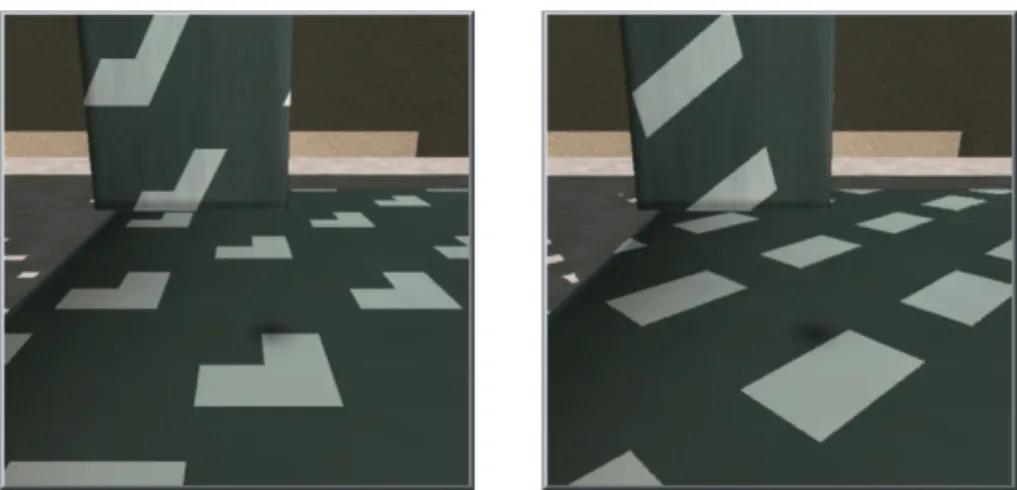
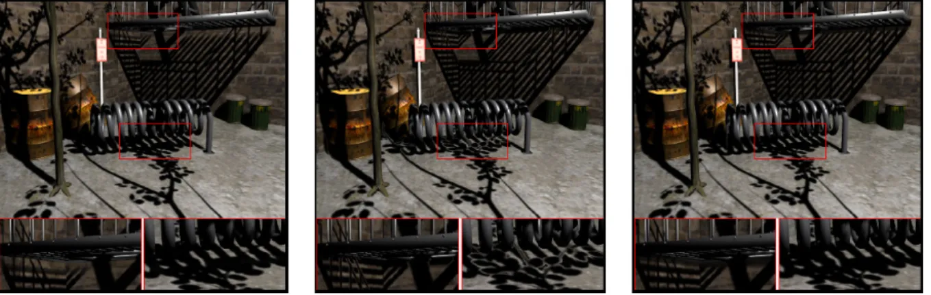
Shadow mapping has been one of the most used algorithms for real time calculation of shadows, since it is extremely simple and quick in calculating said shadows, but not always presents the best results. On the other hand, ray-tracing presents pixel-perfect shadows, but it is more demanding from a computational point of view.
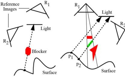
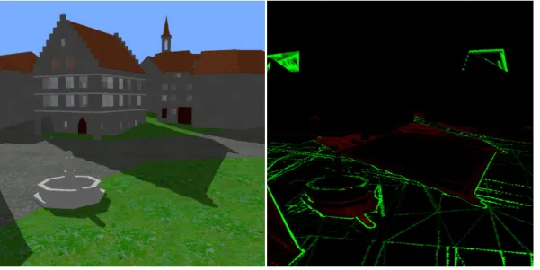
Shadow mapping has seen many proposals to increase its accuracy, while retaining its high performance nature. Some of the methods proposed, based solely on the standard shadow mapping technique, do improve significantly the standard shadow mapping result at the expense of a minor decrease in performance. Other approaches propose hybrid methods, using shadow mapping as a way of limiting the number of pixels that require ray-tracing. One of such approaches uses texel coherence to reduce the number of pixels that require testing.
These latter approaches establish the theme for this work. The goal is to narrow down as much as possible the amount of pixels that require a ray-tracer to determine its shadow status.
The first step was to identify the location of the errors present in a shadow map. The tests confirmed the intuition that most of these errors should be located in the contours of the shadow areas.
The next step focuses on these contour areas and looks for ways to determine the correctness of a pixel’s shadow status. Several methods were proposed to achieve this goal. Some methods were capable of confirming pixels in shadow. Some were capable of correcting pixels in light.
Each method, with the exception of texel coherence, uses a very selective ray-tracer, i.e. only very few triangles are tested for intersection with a single light ray.
Since each method has its strengths and weaknesses an algorithm was proposed, chaining all these methods together. The first step is to determine the set of pixels in the contours of the shadow areas. Then each method is applied in turn, so that only the pixels the remaining unconfirmed/uncorrected pass on to the next stage.
At the end of the algorithm a very large percentage of pixels in shadow were confirmed and a significant number of pixels in light were corrected. The remaining pixels could then be fed to a full ray-tracer. The load of the ray-tracer is severely reduced under this approach making it an affordable solution to obtain pixel perfect shadows in the contours of the shadowed areas.
SHADOW MAPPING E RAY-TRACING
RESUMO
O shadow mapping tem sido um dos algoritmos mais utilizados para o cálculo de sombras em tempo real, já que é extremamente simples e rápido em calcular estas sombras, mas nem sempre apresenta os melhores resultados. Por outro lado, ray-tracing apresenta sombras perfeitas ao nível do pixel mas é mais exigente de um ponto de vista computacional.
Têm havido muitas propostas para o aumento de qualidade do shadow mapping sem afectar o seu desempenho. Alguns dos métodos propostos, baseados somente na técnica de shadow mapping padrão, de facto melhoram significativamente o resultado do shadow mapping padrão ao custo de uma pequena diminuição no desempenho. Outras abordagens propõem métodos híbridos, usando o shadow mapping para limitar o número de pixéis que requerem ray-tracing. Uma destas abordagens usa o texel coherence para reduzir o número de pixéis que precisam de ser testados.
Estas últimas abordagens estabelecem o tema deste trabalho. O objectivo é limitar o máximo possível a quantidade de pixéis que requerem um ray-tracer para determinar o seu sombreamento.
O primeiro passo foi identificar a localização dos erros presentes num shadow map. Os testes confirmaram a intuição de que a maior parte destes erros se deveriam encontrar nos contornos das zonas sombreadas.
O próximo passo foca-se nestas áreas de contorno e procura maneiras de determinar se o sombreamento de um pixel está correcto. Vários métodos foram propostos para conseguir este objectivo. Alguns métodos foram capazes de confirmar pixéis em sombra. Alguns foram capazes de corrigir pixéis em luz.
Cada método, com a excepção do texel coherence, usa um ray-tracer muito selectivo, isto é, apenas uma muito pequena quantidade de triângulos é testada para intersecção com cada raio de luz.
Como cada método tem as suas vantagens e desvantagens um algoritmo que encadeia todos estes métodos foi proposto. O primeiro passo é determinar o conjunto de pixéis nos contornos das áreas sombreadas. Depois cada método é aplicado à vez de modo a que os pixéis que se mantêm por confirmar ou corrigir passem para o próximo passo.
No fim do algoritmo uma grande percentagem de pixéis em sombra foi confirmada e um número significativo de pixéis em luz foi corrigido. O resto dos pixéis poderia então passar por um ray-tracer completo. A carga do ray-tracer é severamente reduzida sob esta abordagem tornando-o numa solução acessível à obtenção de sombras perfeitas ao nível do pixel nos contornos das áreas sombreadas.
TABLE OF CONTENTS
1. INTRODUCTION ... 1 1.1. Motivation ... 2 1.2. Goals... 2 1.3. Methodology ... 3 1.4. Thesis Structure ... 42. STATE OF THE ART ... 5
2.1. Shadow Mapping... 5
2.1.1. Shadow Mapping Basics ... 5
2.1.2. Shadow Mapping Problems ... 6
2.1.3. Shadow Mapping Approaches ... 8
2.2. Ray-Tracing ... 13
2.2.1. Ray-Tracing Basics ... 13
2.3. Combining Both ... 15
2.3.1. Coherence-Based Ray-Tracing ... 15
2.3.2. Hybrid GPU Rendering Pipeline for Alias-Free Hard Shadows ... 16
2.3.3. Hybrid GPU-CPU Renderer ... 18
2.4. Conclusion ... 19
3. ALGORITHM DESCRIPTION ... 21
3.1. Shadow Mapping Errors... 21
3.1.1. Shadow Status and Errors ... 21
3.1.2. Error Location ... 23
3.2. Using Texel Information ... 24
3.3. Using the Information of the Neighbouring Texels ... 28
3.4. Using Texel Coherence ... 31
3.6. Putting It All Together ... 37
3.7. Conclusion ... 41
4. ALGORITHM TESTING ... 43
4.1. Test Scenes ... 44
4.2. Ray-Tracer ... 46
4.3. Shadow Mapping Errors... 52
4.4. Using Texel Coherence ... 55
4.5. Using Texel Information ... 60
4.6. Using the Information of the Neighbours of the Texel ... 63
4.7. Using Geometric Adjacency Information ... 67
4.8. Putting It All Together ... 71
4.9. Final Observations... 76
5. CONCLUSIONS AND FUTURE WORK ... 81
6. BIBLIOGRAPHY ... 85
FIGURE INDEX
Figure 1: How a Shadow Map works. ... 6
Figure 2: The shadow of the tree presents aliasing. ... 6
Figure 3: Perspective Shadow Map example. ... 8
Figure 4: Light Space Perspective Shadow Map example. ... 9
Figure 5: Trapezoidal Shadow Mapping movement flickering. ... 10
Figure 6: Adaptive Shadow map result compared to a shadow mapping result (2048x2048 shadow map versus an effective 524288x524288 shadow map result). ... 10
Figure 7: Parallel-Split Shadow Maps example... 11
Figure 8: Variance Shadow Map light leaking example. ... 12
Figure 9: Comparison between Convoluted, Variance and Exponential Shadow Maps respectively. ... 12
Figure 10: Simple example of Ray-Tracing... 14
Figure 11: Reference image examples for the coherence based ray-tracing. ... 16
Figure 12: Resizing the triangle by moving its edges. ... 17
Figure 13: Example of the uncertain areas when using the Hybrid GPU Rendering Pipeline for Alias-Free Hard Shadows... 18
Figure 14: Green pixels mark where shadow mapping samples disagree in the Hybrid GPU-CPU Renderer. ... 19
Figure 15: Correctly (in green) and incorrectly (in blue) shadowed points by shadow mapping... 22
Figure 16: Correctly (in green) and incorrectly (in blue) lit points by shadow mapping. ... 23
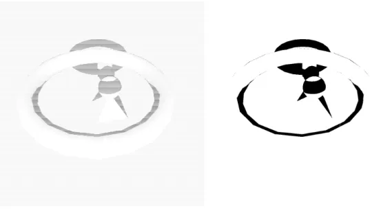
Figure 17: Marked contours and errors of the scene. ... 24
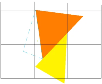
Figure 18: Cases of using texel information. ... 25
Figure 19: Correcting a point wrongly defined in light with the triangle stored in the projected texel. ... 26
Figure 20: Pixel confirmation using texel information. ... 27
Figure 21: The two cases of neighbouring texels. ... 28
Figure 22: Cases using neighbouring texel information with a triangle stored in the centre texel. ... 29
Figure 23: Cases using neighbouring texel information without a triangle stored in the centre texel. ... 30
Figure 24: Pixel confirmation using neighbouring texel information with 8 neighbours. ... 31
Figure 25: Examples of PCF results. ... 32
Figure 26: Pixel confirmation using PCF with four texels. ... 33
Figure 27: Using adjacent geometry information for case a). ... 35
Figure 28: Using adjacent geometry information for case b). ... 35
Figure 29: Correcting a point wrongly defined in light using triangle adjacency. ... 36
Figure 30: Pixel confirmation using geometry adjacency information with 2 levels of adjacency... 37
Figure 31: Average of corrected/confirmed/hinted contour pixels by each method: a) contour pixels; b) shadow map results separated in shadow (black) and light (white); c) errors of the shadow map (gray); d) correct (blue) and incorrect (red) hints using texel coherence; e) confirmed shadow (dark green) and corrected light (light green) pixels by neighbouring texels; f) confirmed shadow pixels (orange) by adjacent geometry. ... 38
Figure 32: Average of corrected/confirmed/hinted contour pixels by the chaining of methods: a) contour pixels; b) shadow map results separated in shadow (black) and light (white); c) errors of the shadow map (gray); d) correct (blue) and incorrect (red) hints using texel coherence; e) confirmed shadow (dark green) and corrected light (light green) pixels by neighbouring texels; f) confirmed shadow pixels (orange) by adjacent geometry; g) non-hinted/uncorrected/unconfirmed pixels (yellow). ... 40
Figure 33: The side (left), with (centre) and against (right) viewpoints of the first scene. ... 44
Figure 35: The with (left), side (centre) and against (right) viewpoints of the third scene. .... 46
Figure 36: The side (left), against (centre) and with (right) viewpoints of the fourth scene. .. 46
Figure 37: Ray-tracer results for the side viewpoint of the primitives scene. ... 47
Figure 38: Ray-tracer results for the with viewpoint of the primitives scene. ... 47
Figure 39: Ray-tracer results for the against viewpoint of the primitives scene. ... 48
Figure 40: Ray-tracer results for the side viewpoint of the bench scene. ... 48
Figure 41: Ray-tracer results for the with viewpoint of the bench scene. ... 49
Figure 42: Ray-tracer results for the against viewpoint of the bench scene. ... 49
Figure 43: Ray-tracer results for the with viewpoint of the trees scene. ... 50
Figure 44: Ray-tracer results for the side viewpoint of the trees scene. ... 50
Figure 45: Ray-tracer results for the against viewpoint of the trees scene. ... 51
Figure 46: Ray-tracer results for the side viewpoint of the flowers scene. ... 51
Figure 47: Ray-tracer results for the against viewpoint of the flowers scene. ... 52
Figure 48: Ray-tracer results for the with viewpoint of the flowers scene. ... 52
Figure 49: Best case of shadow map errors being caught inside contours with a 2048x2048 shadow map. ... 53
Figure 50: Worst case of shadow map errors being caught inside contours with a 2048x2048 shadow map. ... 54
Figure 51: Average case of shadow map errors being caught inside contours. ... 54
Figure 52: Average shadow map results separated by contour thickness with a 1024x1024 shadow map (top) and a 2048x2048 shadow map (bottom). ... 55
Figure 53: Best case of texel coherence confirmation using four texels and a 2048x2048 shadow map. ... 56
Figure 54: Worst case of texel coherence confirmation using four texels and a 2048x2048 shadow map. ... 57
Figure 55: Average case of texel coherence confirmation using four texels. ... 58 Figure 56: Best case of texel coherence confirmation using nine texels and a 2048x2048 shadow map. ... 59 Figure 57: Worst case of texel coherence confirmation using nine texels and a 2048x2048 shadow map. ... 59 Figure 58: Average case of texel coherence confirmation using nine texels. ... 60 Figure 59: Average results of texel coherence with four texels separated by contour thickness with a 1024x1024 shadow map (top) and a 2048x2048 shadow map (bottom). ... 60 Figure 60: Best case of only using centre texel information with a 2048x2048 shadow map. 61 Figure 61: Worst case of using centre texel information by itself with a 2048x2048 shadow map. ... 62 Figure 62: Average case of using centre texel information by itself. ... 62 Figure 63: Best case of only using information of four neighbouring texels with a 2048x2048 shadow map. ... 64 Figure 64: Best case of only using information of nine neighbouring texels with a 2048x2048 shadow map. ... 64 Figure 65: Worst case of only using information of four neighbouring texels with a 2048x2048 shadow map. ... 65 Figure 66: Worst case of only information of nine neighbouring texels with a 2048x2048 shadow map. ... 65 Figure 67: Average case of only using information of four neighbouring texels. ... 66 Figure 68: Average case of only using information of nine neighbouring texels. ... 66 Figure 69: Average results of neighbouring texels with nine texels separated by contour thickness with a 1024x1024 shadow map (top) and a 2048x2048 shadow map (bottom). ... 67 Figure 70: Best case of only using centre and first level of adjacent geometry information with a 2048x2048 shadow map... 68
Figure 71: Best case of only using centre and second level of adjacent geometry information with a 2048x2048 shadow map... 68 Figure 72: Worst case of only using centre and first level of adjacent geometry information with a 2048x2048 shadow map... 69 Figure 73: Worst case of only using centre and second level of adjacent geometry information with a 2048x2048 shadow map... 69 Figure 74: Average case of only using centre and first level of adjacent geometry information. ... 70 Figure 75: Average case of only using centre and second level of adjacent geometry information. ... 70 Figure 76: Average results of adjacent geometry with two levels of adjacency separated by contour thickness with a 1024x1024 shadow map (top) and a 2048x2048 shadow map (bottom)... 71 Figure 77: Best case of algorithm pixel confirmation after using information of the neighbouring texels with a 2048x2048 shadow map. ... 72 Figure 78: Worst case of algorithm pixel confirmation after using information of the neighbouring texels with a 2048x2048 shadow map. ... 72 Figure 79: Average case of algorithm pixel confirmation after using information of the neighbouring texels. ... 73 Figure 80: Average results of the algorithm after the neighbouring texel step separated by contour thickness with a 1024x1024 shadow map (top) and a 2048x2048 shadow map (bottom)... 73 Figure 81: Best case of algorithm pixel confirmation after using information of the adjacent geometry with a 2048x2048 shadow map. ... 74 Figure 82: Worst case of algorithm pixel confirmation after using information of the adjacent geometry with a 2048x2048 shadow map. ... 75 Figure 83: Average case of algorithm pixel confirmation after using information of the adjacent geometry. ... 75
Figure 84: Average results of the algorithm after the adjacent geometry step separated by contour thickness with a 1024x1024 shadow map (top) and a 2048x2048 shadow map
(bottom)... 76
Figure 85: Average results of the algorithm after the adjacent geometry step with pixels that were not confirmed, corrected or hinted marked, separated by contour thickness with a 1024x1024 shadow map (top) and a 2048x2048 shadow map (bottom). ... 76
Figure 86: Marked errors of the best case when using a 2048x2048 shadow map. ... 78
Figure 87: Marked errors of the worst case when using a 2048x2048 shadow map. ... 78
Figure 88: Marked errors of the average case. ... 79
Figure 89: Result of the ray-tracing approach for the side viewpoint of the primitives scene. ... 87
Figure 90: Result of the shadow mapping approach for the side viewpoint of the primitives scene. ... 87
Figure 91: Result of texel coherence with four texels for the side viewpoint of the primitives scene. ... 88
Figure 92: Result of texel coherence with nine texels for the side viewpoint of the primitives scene. ... 88
Figure 93: Result of the single texel approach on the side viewpoint of the primitives scene. ... 89
Figure 94: Result of the neighbour texels approach using four neighbours for the side viewpoint of the primitives scene. ... 89
Figure 95: Result of the neighbour texels approach using nine neighbours for the side viewpoint of the primitives scene. ... 90
Figure 96: Result of the adjacent geometry approach with one level of adjacency for the side viewpoint of the primitives scene. ... 90
Figure 97: Result of the adjacent geometry approach with two levels of adjacency for the side viewpoint of the primitives scene. ... 91
Figure 98: Result of the algorithm with a six pixel thick contour and a 2048x2048 resolution shadow map for the side viewpoint of the primitives scene. ... 91 Figure 99: Corrected/confirmed/hinted contour pixels by each method for the side viewpoint of the primitives scene using a 1024x1024 (top) and a 2048x2048 (bottom) resolution shadow map. ... 92 Figure 100: Corrected/confirmed/hinted contour pixels by the chaining of methods for the side viewpoint of the primitives scene using a 1024x1024 (top) and a 2048x2048 (bottom) resolution shadow map. ... 93 Figure 101: Result of the ray-tracing approach for the with viewpoint of the primitives scene. ... 104 Figure 102: Result of the shadow mapping approach for the with viewpoint of the primitives scene. ... 104 Figure 103: Result of texel coherence with four texels for the with viewpoint of the primitives scene. ... 105 Figure 104: Result of texel coherence with nine texels for the with viewpoint of the primitives scene. ... 105 Figure 105: Result of the single texel approach for the with viewpoint of the primitives scene. ... 106 Figure 106: Result of the neighbour texels approach using four neighbours for the with viewpoint of the primitives scene. ... 106 Figure 107: Result of the neighbour texels approach using nine neighbours for the with viewpoint of the primitives scene. ... 107 Figure 108: Result of the adjacent geometry approach with one level of adjacency for the with viewpoint of the primitives scene. ... 107 Figure 109: Result of the adjacent geometry approach with two levels of adjacency for the with viewpoint of the primitives scene. ... 108 Figure 110: Result of the algorithm with a six pixel thick contour and a 2048x2048 resolution shadow map for the with viewpoint of the primitives scene. ... 108
Figure 111: Corrected/confirmed/hinted contour pixels by each method for the with viewpoint of the primitives scene using a 1024x1024 (top) and a 2048x2048 (bottom) resolution shadow map. ... 109 Figure 112: Corrected/confirmed/hinted contour pixels by the chaining of methods for the with viewpoint of the primitives scene using a 1024x1024 (top) and a 2048x2048 (bottom) resolution shadow map. ... 110 Figure 113: Result of the ray-tracing approach for the against viewpoint of the primitives scene. ... 120 Figure 114: Result of the shadow mapping approach for the against viewpoint of the primitives scene. ... 120 Figure 115: Result of texel coherence with four texels for the against viewpoint of the primitives scene. ... 121 Figure 116: Result of texel coherence with nine texels for the against viewpoint of the primitives scene. ... 121 Figure 117: Result of the single texel approach for the against viewpoint of the primitives scene. ... 122 Figure 118: Result of the neighbour texels approach using three pixels for the against viewpoint of the primitives scene. ... 122 Figure 119: Result of the neighbour texels approach using eight pixels for the against viewpoint of the primitives scene. ... 123 Figure 120: Result of the adjacent geometry approach with one level of adjacency for the against viewpoint of the primitives scene. ... 123 Figure 121: Result of the adjacent geometry approach with two levels of adjacency for the against viewpoint of the primitives scene. ... 124 Figure 122: Result of the algorithm with a six pixel thick contour and a 2048x2048 resolution shadow map for the against viewpoint of the primitives scene. ... 124
Figure 123: Corrected/confirmed/hinted contour pixels by each method for the against viewpoint of the primitives scene using a 1024x1024 (top) and a 2048x2048 (bottom) resolution shadow map. ... 125 Figure 124: Corrected/confirmed/hinted contour pixels by the chaining of methods for the against viewpoint of the primitives scene using a 1024x1024 (top) and a 2048x2048 (bottom) resolution shadow map. ... 126 Figure 125: Result of the ray-tracing approach for the side viewpoint of the bench scene. .. 136 Figure 126: Result of the shadow mapping approach for the side viewpoint of the bench scene. ... 136 Figure 127: Result of texel coherence with four texels for the side viewpoint of the bench scene. ... 137 Figure 128: Result of texel coherence with nine texels for the side viewpoint of the bench scene. ... 137 Figure 129: Result of the single texel approach for the side viewpoint of the bench scene. . 138 Figure 130: Result of the neighbour texels approach with four neighbours for the side viewpoint of the bench scene. ... 138 Figure 131: Result of the neighbour texels approach with nine neighbours for the side viewpoint of the bench scene. ... 139 Figure 132: Result of the adjacent geometry approach with one level of adjacency for the side viewpoint of the bench scene. ... 139 Figure 133: Result of the adjacent geometry approach with two levels of adjacency for the side viewpoint of the bench scene. ... 140 Figure 134: Result of the algorithm with a six pixel thick contour and a 2048x2048 resolution shadow map for the side viewpoint of the bench scene. ... 140 Figure 135: Corrected/confirmed/hinted contour pixels by each method for the side viewpoint of the bench scene using a 1024x1024 (top) and a 2048x2048 (bottom) resolution shadow map. ... 141
Figure 136: Corrected/confirmed/hinted contour pixels by the chaining of methods for the side viewpoint of the bench scene using a 1024x1024 (top) and a 2048x2048 (bottom) resolution shadow map. ... 142 Figure 137: Result of the ray-tracing approach for the with viewpoint of the bench scene. . 152 Figure 138: Result of the shadow mapping approach for the with viewpoint of the bench scene. ... 152 Figure 139: Result of texel coherence with four texels for the with viewpoint of the bench scene. ... 153 Figure 140: Result of texel coherence with nine texels for the with viewpoint of the bench scene. ... 153 Figure 141: Result of the single texel approach for the with viewpoint of the bench scene. 154 Figure 142: Result of the neighbour texels approach with four neighbours for the with viewpoint of the bench scene. ... 154 Figure 143: Result of the neighbour texels approach with nine neighbours for the with viewpoint of the bench scene. ... 155 Figure 144: Result of the adjacent geometry approach with one level of adjacency for the with viewpoint of the bench scene. ... 155 Figure 145: Result of the adjacent geometry approach with two levels of adjacency for the with viewpoint of the bench scene. ... 156 Figure 146: Result of the algorithm with a six pixel thick contour and a 2048x2048 resolution shadow map for the with viewpoint of the bench scene. ... 156 Figure 147: Corrected/confirmed/hinted contour pixels by each method for the with viewpoint of the bench scene using a 1024x1024 (top) and a 2048x2048 (bottom) resolution shadow map. ... 157 Figure 148: Corrected/confirmed/hinted contour pixels by the chaining of methods for the with viewpoint of the bench scene using a 1024x1024 (top) and a 2048x2048 (bottom) resolution shadow map. ... 158
Figure 149: Result of the ray-tracing approach for the against viewpoint of the bench scene. ... 168 Figure 150: Result of the shadow mapping approach for the against viewpoint of the bench scene. ... 168 Figure 151: Result of texel coherence with four texels for the against viewpoint of the bench scene. ... 169 Figure 152: Result of texel coherence with nine texels for the against viewpoint of the bench scene. ... 169 Figure 153: Result of the single texel approach for the against viewpoint of the bench scene. ... 170 Figure 154: Result of the neighbour texels approach using four neighbours for the against viewpoint of the bench scene. ... 170 Figure 155: Result of the neighbour texels approach using nine neighbours for the against viewpoint of the bench scene. ... 171 Figure 156: Result of the adjacent geometry approach with one level of adjacency for the against viewpoint of the bench scene... 171 Figure 157: Result of the adjacent geometry approach with two levels of adjacency for the against viewpoint of the bench scene... 172 Figure 158: Result of the algorithm with a six pixel thick contour and a 2048x2048 resolution shadow map for the against viewpoint of the bench scene. ... 172 Figure 159: Corrected/confirmed/hinted contour pixels by each method for the against viewpoint of the bench scene using a 1024x1024 (top) and a 2048x2048 (bottom) resolution shadow map. ... 173 Figure 160: Corrected/confirmed/hinted contour pixels by the chaining of methods for the against viewpoint of the bench scene using a 1024x1024 (left) and a 2048x2048 (bottom) resolution shadow map. ... 174 Figure 161: Result of the ray-tracing approach for the with viewpoint of the trees scene. ... 186
Figure 162: Result of the shadow mapping approach for the with viewpoint of the trees scene. ... 186 Figure 163: Result of texel coherence with four texels for the with viewpoint of the trees scene. ... 187 Figure 164: Result of texel coherence with nine texels for the with viewpoint of the trees scene. ... 187 Figure 165: Result of the single texel approach for the with viewpoint of the trees scene. .. 188 Figure 166: Result of the neighbour texels approach using four neighbours for the with viewpoint of the trees scene. ... 188 Figure 167: Result of the neighbour texels approach using nine neighbours for the with viewpoint of the trees scene. ... 189 Figure 168: Result of the adjacent geometry approach with one level of adjacency for the with viewpoint of the trees scene. ... 189 Figure 169: Result of the adjacent geometry approach with two levels of adjacency for the with viewpoint of the trees scene. ... 190 Figure 170: Result of the algorithm with a six pixel thick contour and a 2048x2048 resolution shadow map for the with viewpoint of the trees scene. ... 190 Figure 171: Corrected/confirmed/hinted contour pixels by each method for the with viewpoint of the trees scene using a 1024x1024 (top) and a 2048x2048 (bottom) resolution shadow map. ... 191 Figure 172: Corrected/confirmed/hinted contour pixels by the chaining of methods for the with viewpoint of the trees scene using a 1024x1024 (top) and a 2048x2048 (bottom) resolution shadow map. ... 192 Figure 173: Result of the ray-tracing approach for the side viewpoint of the trees scene. .... 203 Figure 174: Result of the shadow mapping approach for the side viewpoint of the trees scene. ... 203
Figure 175: Result of texel coherence with four texels for the side viewpoint of the trees scene. ... 204 Figure 176: Result of texel coherence with nine texels for the side viewpoint of the trees scene. ... 204 Figure 177: Result of the single texel approach for the side viewpoint of the trees scene. ... 205 Figure 178: Result of the neighbour texels approach with four neighbours for the side viewpoint of the trees scene. ... 205 Figure 179: Result of the neighbour texels approach with nine neighbours for the side viewpoint of the trees scene. ... 206 Figure 180: Result of the adjacent geometry approach with one level of adjacency for the side viewpoint of the trees scene. ... 206 Figure 181: Result of the adjacent geometry approach with two levels of adjacency for the side viewpoint of the trees scene. ... 207 Figure 182: Result of the algorithm with a six pixel thick contour and a 2048x2048 resolution shadow map for the side viewpoint of the trees scene. ... 207 Figure 183: Corrected/confirmed/hinted contour pixels by each method for the side viewpoint of the trees scene using a 1024x1024 (top) and a 2048x2048 (bottom) resolution shadow map. ... 208 Figure 184: Corrected/confirmed/hinted contour pixels by the chaining of methods for the side viewpoint of the trees scene using a 1024x1024 (top) and a 2048x2048 (bottom) resolution shadow map. ... 209 Figure 185: Result of the ray-tracing approach for the against viewpoint of the trees scene. ... 219 Figure 186: Result of the shadow mapping approach for the against viewpoint of the trees scene. ... 219 Figure 187: Result of texel coherence with four texels for the against viewpoint of the trees scene. ... 220
Figure 188: Result of texel coherence with nine texels for the against viewpoint of the trees scene. ... 220 Figure 189: Result of the single texel approach for the against viewpoint of the trees scene. ... 221 Figure 190: Result of the neighbour texels approach using four neighbours for the against viewpoint of the trees scene. ... 221 Figure 191: Result of the neighbour texels approach using nine neighbours for the against viewpoint of the trees scene. ... 222 Figure 192: Result of the adjacent geometry approach with one level of adjacency for the against viewpoint of the trees scene... 222 Figure 193: Result of the adjacent geometry approach with two level of adjacency for the against viewpoint of the trees scene... 223 Figure 194: Result of the algorithm with a six pixel thick contour and a 2048x2048 resolution shadow map for the against viewpoint of the trees scene. ... 223 Figure 195: Corrected/confirmed/hinted contour pixels by each method for the against viewpoint of the trees scene using a 1024x1024 (top) and a 2048x2048 (bottom) resolution shadow map. ... 224 Figure 196: Corrected/confirmed/hinted contour pixels by the chaining of methods for the against viewpoint of the trees scene using a 1024x1024 (top) and a 2048x2048 (bottom) resolution shadow map. ... 225 Figure 197: Result of the ray-tracing approach for the side viewpoint of the flowers scene.235 Figure 198: Result of the shadow mapping approach for the side viewpoint of the flowers scene. ... 235 Figure 199: Result of texel coherence with four texels for the side viewpoint of the flowers scene. ... 236 Figure 200: Result of texel coherence with nine texels for the side viewpoint of the flowers scene. ... 236
Figure 201: Result of the single texel approach for the side viewpoint of the flowers scene. ... 237 Figure 202: Result of the neighbour texels approach using four neighbours for the side viewpoint of the flowers scene. ... 237 Figure 203: Result of the neighbour texels approach using nine neighbours for the side viewpoint of the flowers scene. ... 238 Figure 204: Result of the adjacent geometry approach with one level of adjacency for the side viewpoint of the flowers scene. ... 238 Figure 205: Result of the adjacent geometry approach with two levels of adjacency for the side viewpoint of the flowers scene. ... 239 Figure 206: Result of the algorithm with a six pixel thick contour and a 2048x2048 resolution shadow map for the side viewpoint of the flowers scene. ... 239 Figure 207: Corrected/confirmed/hinted contour pixels by each method for the side viewpoint of the flowers scene using a 1024x1024 (top) and a 2048x2048 (bottom) resolution shadow map. ... 240 Figure 208: Corrected/confirmed/hinted contour pixels by the chaining of methods for the side viewpoint of the flowers scene using a 1024x1024 (top) and a 2048x2048 (bottom) resolution shadow map. ... 241 Figure 209: Result of the ray-tracing approach for the against viewpoint of the flowers scene. ... 253 Figure 210: Result of the shadow mapping approach for the against viewpoint of the flowers scene. ... 253 Figure 211: Result of texel coherence with four texels for the against viewpoint of the flowers scene. ... 254 Figure 212: Result of texel coherence with nine texels for the against viewpoint of the flowers scene. ... 254 Figure 213: Result of the single texel approach for the against viewpoint of the flowers scene. ... 255
Figure 214: Result of the neighbour texels approach using four neighbours for the against viewpoint of the flowers scene. ... 255 Figure 215: Result of the neighbour texels approach using nine neighbours for the against viewpoint of the flowers scene. ... 256 Figure 216: Result of the adjacent geometry approach with one level of adjacency for the against viewpoint of the flowers scene. ... 256 Figure 217: Result of the adjacent geometry approach with two levels of adjacency for the against viewpoint of the flowers scene. ... 257 Figure 218: Result of the algorithm with a six pixel thick contour and a 2048x2048 resolution shadow map for the against viewpoint of the flowers scene. ... 257 Figure 219: Corrected/confirmed/hinted contour pixels by each method for the against viewpoint of the flowers scene using a 1024x1024 (top) and a 2048x2048 (bottom) resolution shadow map. ... 258 Figure 220: Corrected/confirmed/hinted contour pixels by the chaining of methods for the against viewpoint of the flowers scene using a 1024x1024 (top) and a 2048x2048 (bottom) resolution shadow map. ... 259 Figure 221: Result of the ray-tracing approach for the with viewpoint of the flowers scene. ... 269 Figure 222: Result of the shadow mapping approach for the with viewpoint of the flowers scene. ... 269 Figure 223: Result of texel coherence with four texels for the with viewpoint of the flowers scene. ... 270 Figure 224: Result of texel coherence with nine texels for the with viewpoint of the flowers scene. ... 270 Figure 225: Result of the single texel approach for the with viewpoint of the flowers scene. ... 271 Figure 226: Result of the neighbour texels approach using four neighbours for the with viewpoint of the flowers scene. ... 271
Figure 227: Result of the neighbour texels approach using nine neighbours for the with viewpoint of the flowers scene. ... 272 Figure 228: Result of the adjacent geometry approach with one level of adjacency for the with viewpoint of the flowers scene. ... 272 Figure 229: Result of the adjacent geometry approach with two levels of adjacency for the with viewpoint of the flowers scene. ... 273 Figure 230: Result of the algorithm with a six pixel thick contour and a 2048x2048 resolution shadow map for the with viewpoint of the flowers scene. ... 273 Figure 231: Corrected/confirmed/hinted contour pixels by each method for the with viewpoint of the flowers scene using a 1024x1024 (top) and a 2048x2048 (bottom) resolution shadow map. ... 274 Figure 232: Corrected/confirmed/hinted contour pixels by the chaining of methods for the with viewpoint of the flowers scene using a 1024x1024 (top) and a 2048x2048 (bottom) resolution shadow map. ... 275
TABLE INDEX
Table 1: Information of the first scene. ... 44 Table 2: Information of the second scene. ... 45 Table 3: Information of the third scene. ... 45 Table 4: Information of the fourth scene. ... 46 Table 5: Percentages of errors inside the contours. ... 53 Table 6: Percentage of contour pixels that are incorrect. ... 55 Table 7: Percentage of confirmations by PCF with four texels. ... 56 Table 8: Percentage of confirmations by PCF with nine texels. ... 58 Table 9: Percentage of errors by only using the information of the centre texel. ... 61 Table 10: Percentage of errors by only using the information of the centre and neighbouring texels. ... 63 Table 11: Percentage of errors by only using the information of the centre texel and the adjacent geometry. ... 67 Table 12: Percentage of confirmations by algorithm after using neighbouring texel information. ... 71 Table 13: Percentage of confirmations by algorithm after using adjacent geometry information. ... 74 Table 14: Percentage of wrong confirmations after applying the algorithm and ray-tracing uncertain pixels. ... 77 Table 15: Percentage of wrongly defined pixels if uncertain pixels after algorithm are left in light. ... 77 Table 16: Difference between the approaches that use ray-tracing and the actual ray-tracer for the side viewpoint of the primitives scene. ... 94 Table 17: Wrongly defined pixels in the shadow mapping result which are inside the contour in the side viewpoint of the primitives scene. ... 94
Table 18: Pixels that the shadow map defines wrongly in the side viewpoint of the primitives scene, separated in pixels defined in light and in shadow, compared to the total amount of pixels lighted in the same way. ... 95 Table 19: Pixel confirmation when using texel coherence with four texels for the side viewpoint of the primitives scene. ... 95 Table 20: Pixel shadowing for pixels that don’t achieve texel coherence with four texels for the side viewpoint of the primitives scene. ... 96 Table 21: Pixel confirmation when using texel coherence with nine texels for the side viewpoint of the primitives scene. ... 96 Table 22: Pixel shadowing for pixels that don’t achieve texel coherence with nine texels for the side viewpoint of the primitives scene. ... 97 Table 23: Pixel correction between the single texel approach and the shadow mapping approach for the side viewpoint of the primitives scene... 98 Table 24: Pixel correction between the neighbour texels approach and the shadow mapping approach for the side viewpoint of the primitives scene... 98 Table 25: Average of triangle intersections when using the neighbour texels approach for the side viewpoint of the primitives scene. ... 99 Table 26: Pixel correction between the adjacent geometry approach and the shadow mapping approach for the side viewpoint of the primitives scene... 100 Table 27: Average of triangle intersections when using the adjacent geometry approach for the side viewpoint of the primitives scene. ... 101 Table 28: Pixel correction by the neighbour texels (9 texels) and the adjacent geometry (2 levels) approaches separated by lighting change for the side viewpoint of the primitives scene. ... 102 Table 29: Algorithm results of the side viewpoint of the primitives scene. ... 103 Table 30: Difference between the approaches that use ray-tracing and the actual ray-tracer for the with viewpoint of the primitives scene. ... 111
Table 31: Wrongly defined pixels in the shadow mapping result which are inside the contour in the with viewpoint of the primitives scene. ... 111 Table 32: Pixels that the shadow map defines wrongly in the with viewpoint of the primitives scene, separated in pixels defined in light and in shadow, compared to the total amount of pixels lighted in the same way. ... 112 Table 33: Pixel confirmation when using texel coherence with four texels for the with viewpoint of the primitives scene. ... 112 Table 34: Pixel shadowing for pixels that don’t achieve texel coherence with four texels for the with viewpoint of the primitives scene. ... 113 Table 35: Pixel confirmation when using texel coherence with nine texels for the with viewpoint of the primitives scene. ... 113 Table 36: Pixel shadowing for pixels that don’t achieve texel coherence with nine texels for the with viewpoint of the primitives scene. ... 114 Table 37: Pixel correction between the single texel approach and the shadow mapping approach for the with viewpoint of the primitives scene. ... 115 Table 38: Pixel correction between the neighbour texels approach using four neighbours and the shadow mapping approach for the with viewpoint of the primitives scene. ... 115 Table 39: Pixel correction between the neighbour texels approach using nine neighbours and the shadow mapping approach for the with viewpoint of the primitives scene. ... 115 Table 40: Average of triangle intersections when using the neighbour texels approach for the with viewpoint of the primitives scene. ... 116 Table 41: Pixel correction between the adjacent geometry approach with one level of adjacency and the shadow mapping approach for the with viewpoint of the primitives scene. ... 116 Table 42: Pixel correction between the adjacent geometry approach with two levels of adjacency and the shadow mapping approach for the with viewpoint of the primitives scene. ... 116
Table 43: Average of triangle intersections when using the adjacent geometry approach for the with viewpoint of the primitives scene. ... 117 Table 44: Pixel correction by the neighbour texels (9 texels) and the adjacent geometry (2 levels) approaches separated by lighting change for the with viewpoint of the primitives scene. ... 118 Table 45: Algorithm results of the with viewpoint of the primitives scene... 119 Table 46: Difference between the approaches that use ray-tracing and the actual ray-tracer for the against viewpoint of the primitives scene. ... 127 Table 47: Wrongly defined pixels in the shadow mapping result which are inside the contour in the against viewpoint of the primitives scene. ... 127 Table 48: Pixels that the shadow map defines wrongly in the against viewpoint of the primitives scene, separated in pixels defined in light and in shadow, compared to the total amount of pixels lighted in the same way. ... 128 Table 49: Pixel confirmation when using texel coherence with four texels for the against viewpoint of the primitives scene. ... 128 Table 50: Pixel shadowing for pixels that don’t achieve texel coherence with four texels for the against viewpoint of the primitives scene. ... 129 Table 51: Pixel confirmation when using texel coherence with nine texels for the against viewpoint of the primitives scene. ... 129 Table 52: Pixel shadowing for pixels that don’t achieve texel coherence with nine texels for the against viewpoint of the primitives scene. ... 130 Table 53: Pixel correction between the single texel approach and the shadow mapping approach for the against viewpoint of the primitives scene. ... 131 Table 54: Pixel correction between the neighbour texels approach using four neighbours and the shadow mapping approach for the against viewpoint of the primitives scene. ... 131 Table 55: Pixel correction between the neighbour texels approach using nine neighbours and the shadow mapping approach for the against viewpoint of the primitives scene. ... 131
Table 56: Average of triangle intersections when using the neighbour texels approach for the against viewpoint of the primitives scene. ... 132 Table 57: Pixel correction between the adjacent geometry approach with one level of adjacency and the shadow mapping approach for the against viewpoint of the primitives scene. ... 132 Table 58: Pixel correction between the adjacent geometry approach with two levels of adjacency and the shadow mapping approach for the against viewpoint of the primitives scene. ... 132 Table 59: Average of triangle intersections when using the adjacent geometry approach for the against viewpoint of the primitives scene. ... 133 Table 60: Pixel correction by the neighbour texels (9 texels) and the adjacent geometry (2 levels) approaches separated by lighting change for the against viewpoint of the primitives scene. ... 134 Table 61: Algorithm results of the against viewpoint of the primitives scene. ... 135 Table 62: Difference between the approaches that use ray-tracing and the actual ray-tracer for the side viewpoint of the bench scene... 143 Table 63: Wrongly defined pixels in the shadow mapping result which are inside the contour in the side viewpoint of the bench scene. ... 143 Table 64: Pixels that the shadow map defines wrongly in the side viewpoint of the bench scene, separated in pixels defined in light and in shadow, compared to the total amount of pixels lighted in the same way. ... 144 Table 65: Pixel confirmation when using texel coherence with four texels for the side viewpoint of the bench scene. ... 144 Table 66: Pixel shadowing for pixels that don’t achieve texel coherence with four texels for the side viewpoint of the bench scene... 145 Table 67: Pixel confirmation when using texel coherence with nine texels for the side viewpoint of the bench scene. ... 145
Table 68: Pixel shadowing for pixels that don’t achieve texel coherence with nine texels for the side viewpoint of the bench scene... 146 Table 69: Pixel correction between the single texel approach and the shadow mapping approach for the side viewpoint of the bench scene. ... 147 Table 70: Pixel correction between the neighbour texels approach using four neighbours and the shadow mapping approach for the side viewpoint of the bench scene. ... 147 Table 71: Pixel correction between the neighbour texels approach using nine neighbours and the shadow mapping approach for the side viewpoint of the bench scene. ... 147 Table 72: Average of triangle intersections when using the neighbour texels approach for the side viewpoint of the bench scene. ... 148 Table 73: Pixel correction between the adjacent geometry approach with one level of adjacency and the shadow mapping approach for the side viewpoint of the bench scene. ... 148 Table 74: Pixel correction between the adjacent geometry approach with two levels of adjacency and the shadow mapping approach for the side viewpoint of the bench scene. ... 148 Table 75: Average of triangle intersections when using the adjacent geometry approach for the side viewpoint of the bench scene... 149 Table 76: Pixel correction by the neighbour texels (9 texels) and the adjacent geometry (2 levels) approaches separated by lighting change for the side viewpoint of the bench scene. 150 Table 77: Algorithm results of the side viewpoint of the bench scene. ... 151 Table 78: Difference between the approaches that use ray-tracing and the actual ray-tracer for the with viewpoint of the bench scene. ... 159 Table 79: Wrongly defined pixels in the shadow mapping result which are inside the contour in the with viewpoint of the bench scene. ... 159 Table 80: Pixels that the shadow map defines wrongly in the with viewpoint of the bench scene, separated in pixels defined in light and in shadow, compared to the total amount of pixels lighted in the same way. ... 160
Table 81: Pixel confirmation when using texel coherence with four texels for the with viewpoint of the bench scene. ... 160 Table 82: Pixel shadowing for pixels that don’t achieve texel coherence with four texels for the with viewpoint of the bench scene. ... 161 Table 83: Pixel confirmation when using texel coherence with nine texels for the with viewpoint of the bench scene. ... 161 Table 84: Pixel shadowing for pixels that don’t achieve texel coherence with nine texels for the with viewpoint of the bench scene. ... 162 Table 85: Pixel correction between the single texel approach and the shadow mapping approach for the with viewpoint of the bench scene. ... 163 Table 86: Pixel correction between the neighbour texels approach using four neighbours and the shadow mapping approach for the with viewpoint of the bench scene. ... 163 Table 87: Pixel correction between the neighbour texels approach using nine neighboursand the shadow mapping approach for the with viewpoint of the bench scene. ... 163 Table 88: Average of triangle intersections when using the neighbour texels approach for the with viewpoint of the bench scene. ... 164 Table 89: Pixel correction between the adjacent geometry approach with one level of adjacency and the shadow mapping approach for the with viewpoint of the bench scene. ... 164 Table 90: Pixel correction between the adjacent geometry approach with two levels of adjacency and the shadow mapping approach for the with viewpoint of the bench scene. ... 164 Table 91: Average of triangle intersections when using the adjacent geometry approach for the with viewpoint of the bench scene. ... 165 Table 92: Pixel correction by the neighbour texels (9 texels) and the adjacent geometry (2 levels) approaches separated by lighting change for the with viewpoint of the bench scene. ... 166 Table 93: Algorithm results of the with viewpoint of the bench scene. ... 167
Table 94: Difference between the approaches that use ray-tracing and the actual ray-tracer for the against viewpoint of the bench scene. ... 175 Table 95: Wrongly defined pixels in the shadow mapping result which are inside the contour in the against viewpoint of the bench scene. ... 175 Table 96: Pixels that the shadow map defines wrongly in the against viewpoint of the bench scene, separated in pixels defined in light and in shadow, compared to the total amount of pixels lighted in the same way. ... 176 Table 97: Pixel confirmation when using texel coherence with four texels for the against viewpoint of the bench scene. ... 176 Table 98: Pixel shadowing for pixels that don’t achieve texel coherence with four texels for the against viewpoint of the bench scene. ... 177 Table 99: Pixel confirmation when using texel coherence with nine texels for the against viewpoint of the bench scene. ... 177 Table 100: Pixel shadowing for pixels that don’t achieve texel coherence with nine texels for the against viewpoint of the bench scene. ... 178 Table 101: Pixel correction between the single texel approach and the shadow mapping approach for the against viewpoint of the bench scene. ... 179 Table 102: Pixel correction between the neighbour texels approach and the shadow mapping approach for the against viewpoint of the bench scene. ... 180 Table 103: Average of triangle intersections when using the neighbour texels approach for the against viewpoint of the bench scene. ... 181 Table 104: Pixel correction between the adjacent geometry approach and the shadow mapping approach for the against viewpoint of the bench scene. ... 182 Table 105: Average of triangle intersections when using the adjacent geometry approach for the against viewpoint of the bench scene. ... 183 Table 106: Pixel correction by the neighbour texels (9 texels) and the adjacent geometry (2 levels) approaches separated by lighting change for the against viewpoint of the bench scene. ... 184
Table 107: Algorithm results of the against viewpoint of the bench scene. ... 185 Table 108: Difference between the approaches that use ray-tracing and the actual ray-tracer for the with viewpoint of the trees scene. ... 193 Table 109: Wrongly defined pixels in the shadow mapping result which are inside the contour in the with viewpoint of the trees scene. ... 193 Table 110: Pixels that the shadow map defines wrongly in the with viewpoint of the trees scene, separated in pixels defined in light and in shadow, compared to the total amount of pixels lighted in the same way. ... 194 Table 111: Pixel confirmation when using texel coherence with four texels for the with viewpoint of the trees scene. ... 194 Table 112: Pixel shadowing for pixels that don’t achieve texel coherence with four texels for the with viewpoint of the trees scene. ... 195 Table 113: Pixel confirmation when using texel coherence with nine texels for the with viewpoint of the trees scene. ... 195 Table 114: Pixel shadowing for pixels that don’t achieve texel coherence with nine texels for the with viewpoint of the trees scene. ... 196 Table 115: Pixel correction between the single texel approach and the shadow mapping approach for the with viewpoint of the trees scene. ... 197 Table 116: Pixel correction between the neighbour texels approach and the shadow mapping approach for the with viewpoint of the trees scene. ... 197 Table 117: Average of triangle intersections when using the neighbour texels approach for the with viewpoint of the trees scene. ... 198 Table 118: Pixel correction between the adjacent geometry approach and the shadow mapping approach for the with viewpoint of the trees scene... 199 Table 119: Average of triangle intersections when using the adjacent geometry approach for the with viewpoint of the trees scene. ... 200
Table 120: Pixel correction by the neighbour texels (9 texels) and the adjacent geometry (2 levels) approaches separated by lighting change for the with viewpoint of the trees scene. . 201 Table 121: Algorithm results of the with viewpoint of the trees scene. ... 202 Table 122: Difference between the approaches that use ray-tracing and the actual ray-tracer for the side viewpoint of the trees scene. ... 210 Table 123: Wrongly defined pixels in the shadow mapping result which are inside the contour in the side viewpoint of the trees scene. ... 210 Table 124: Pixels that the shadow map defines wrongly in the side viewpoint of the trees scene, separated in pixels defined in light and in shadow, compared to the total amount of pixels lighted in the same way. ... 211 Table 125: Pixel confirmation when using texel coherence with four texels for the side viewpoint of the trees scene. ... 211 Table 126: Pixel shadowing for pixels that don’t achieve texel coherence with four texels for the side viewpoint of the trees scene... 212 Table 127: Pixel confirmation when using texel coherence with nine texels for the side viewpoint of the trees scene. ... 212 Table 128: Pixel shadowing for pixels that don’t achieve texel coherence with nine texels for the side viewpoint of the trees scene... 213 Table 129: Pixel correction between the single texel approach and the shadow mapping approach for the side viewpoint of the trees scene. ... 214 Table 130: Pixel correction between the neighbour texels approach using four neighbours and the shadow mapping approach for the side viewpoint of the trees scene. ... 214 Table 131: Pixel correction between the neighbour texels approach using nine neighbours and the shadow mapping approach for the side viewpoint of the trees scene. ... 214 Table 132: Average of triangle intersections when using the neighbour texels approach for the side viewpoint of the trees scene... 215
Table 133: Pixel correction between the adjacent geometry approach with one level of adjacency and the shadow mapping approach for the side viewpoint of the trees scene. ... 215 Table 134: Pixel correction between the adjacent geometry approach with two level of adjacency and the shadow mapping approach for the side viewpoint of the trees scene. ... 215 Table 135: Average of triangle intersections when using the adjacent geometry approach for the side viewpoint of the trees scene... 216 Table 136: Pixel correction by the neighbour texels (9 texels) and the adjacent geometry (2 levels) approaches separated by lighting change for the side viewpoint of the trees scene. . 217 Table 137: Algorithm results of the side viewpoint of the trees scene. ... 218 Table 138: Difference between the approaches that use ray-tracing and the actual ray-tracer for the against viewpoint of the trees scene. ... 226 Table 139: Wrongly defined pixels in the shadow mapping result which are inside the contour in the against viewpoint of the trees scene. ... 226 Table 140: Pixels that the shadow map defines wrongly in the against viewpoint of the trees scene, separated in pixels defined in light and in shadow, compared to the total amount of pixels lighted in the same way. ... 227 Table 141: Pixel confirmation when using texel coherence with four texels for the against viewpoint of the trees scene. ... 227 Table 142: Pixel shadowing for pixels that don’t achieve texel coherence with four texels for the against viewpoint of the trees scene. ... 228 Table 143: Pixel confirmation when using texel coherence with nine texels for the against viewpoint of the trees scene. ... 228 Table 144: Pixel shadowing for pixels that don’t achieve texel coherence with nine texels for the against viewpoint of the trees scene. ... 229 Table 145: Pixel correction between the single texel approach and the shadow mapping approach for the against viewpoint of the trees scene. ... 230
Table 146: Pixel correction between the neighbour texels approach using four neighbours and the shadow mapping approach for the against viewpoint of the trees scene. ... 230 Table 147: Pixel correction between the neighbour texels approach using nine neighbours and the shadow mapping approach for the against viewpoint of the trees scene. ... 230 Table 148: Average of triangle intersections when using the neighbour texels approach for the against viewpoint of the trees scene. ... 231 Table 149: Pixel correction between the adjacent geometry approach with one level of adjacency and the shadow mapping approach for the against viewpoint of the trees scene. 231 Table 150: Pixel correction between the adjacent geometry approach with two level of adjacency and the shadow mapping approach for the against viewpoint of the trees scene. 231 Table 151: Average of triangle intersections when using the adjacent geometry approach for the against viewpoint of the trees scene. ... 232 Table 152: Pixel correction by the neighbour texels (9 texels) and the adjacent geometry (2 levels) approaches separated by lighting change for the against viewpoint of the trees scene. ... 233 Table 153: Algorithm results of the against viewpoint of the trees scene. ... 234 Table 154: Difference between the approaches that use ray-tracing and the actual ray-tracer for the side viewpoint of the flowers scene. ... 242 Table 155: Wrongly defined pixels in the shadow mapping result which are inside the contour in the side viewpoint of the flowers scene. ... 242 Table 156: Pixels that the shadow map defines wrongly in the side viewpoint of the flowers scene, separated in pixels defined in light and in shadow, compared to the total amount of pixels lighted in the same way. ... 243 Table 157: Pixel confirmation when using texel coherence with four texels for the side viewpoint of the flowers scene. ... 243 Table 158: Pixel shadowing for pixels that don’t achieve texel coherence with four texels for the side viewpoint of the flowers scene. ... 244
Table 159: Pixel confirmation when using texel coherence with nine texels for the side viewpoint of the flowers scene. ... 244 Table 160: Pixel shadowing for pixels that don’t achieve texel coherence with nine texels for the side viewpoint of the flowers scene. ... 245 Table 161: Pixel correction between the single texel approach and the shadow mapping approach for the side viewpoint of the flowers scene. ... 246 Table 162: Pixel correction between the neighbour texels approach and the shadow mapping approach for the side viewpoint of the flowers scene. ... 247 Table 163: Average of triangle intersections when using the neighbour texels approach for the side viewpoint of the flowers scene. ... 248 Table 164: Pixel correction between the adjacent geometry approach and the shadow mapping approach for the side viewpoint of the flowers scene. ... 249 Table 165: Average of triangle intersections when using the adjacent geometry approach for the side viewpoint of the flowers scene. ... 250 Table 166: Pixel correction by the neighbour texels (9 texels) and the adjacent geometry (2 levels) approaches separated by lighting change for the side viewpoint of the flowers scene. ... 251 Table 167: Algorithm results of the side viewpoint of the flowers scene. ... 252 Table 168: Difference between the approaches that use ray-tracing and the actual ray-tracer for the against viewpoint of the flowers scene... 260 Table 169: Wrongly defined pixels in the shadow mapping result which are inside the contour in the against viewpoint of the flowers scene. ... 260 Table 170: Pixels that the shadow map defines wrongly in the against viewpoint of the flowers scene, separated in pixels defined in light and in shadow, compared to the total amount of pixels lighted in the same way. ... 261 Table 171: Pixel confirmation when using texel coherence with four texels for the against viewpoint of the flowers scene. ... 261
Table 172: Pixel shadowing for pixels that don’t achieve texel coherence with four texels for the against viewpoint of the flowers scene. ... 262 Table 173: Pixel confirmation when using texel coherence with nine texels for the against viewpoint of the flowers scene. ... 262 Table 174: Pixel shadowing for pixels that don’t achieve texel coherence with nine texels for the against viewpoint of the flowers scene. ... 263 Table 175: Pixel correction between the single texel approach and the shadow mapping approach for the against viewpoint of the flowers scene. ... 264 Table 176: Pixel correction between the neighbour texels approach using four neighbours and the shadow mapping approach for the against viewpoint of the flowers scene. ... 264 Table 177: Pixel correction between the neighbour texels approach using nine neighbours and the shadow mapping approach for the against viewpoint of the flowers scene. ... 264 Table 178: Average of triangle intersections when using the neighbour texels approach for the against viewpoint of the flowers scene. ... 265 Table 179: Pixel correction between the adjacent geometry approach with one level of adjacency and the shadow mapping approach for the against viewpoint of the flowers scene. ... 265 Table 180: Pixel correction between the adjacent geometry approach with two level of adjacency and the shadow mapping approach for the against viewpoint of the flowers scene. ... 265 Table 181: Average of triangle intersections when using the adjacent geometry approach for the against viewpoint of the flowers scene. ... 266 Table 182: Pixel correction by the neighbour texels (9 texels) and the adjacent geometry (2 levels) approaches separated by lighting change for the against viewpoint of the flowers scene. ... 267 Table 183: Algorithm results of the against viewpoint of the flowers scene... 268 Table 184: Difference between the approaches that use ray-tracing and the actual ray-tracer for the with viewpoint of the flowers scene. ... 276
Table 185: Wrongly defined pixels in the shadow mapping result which are inside the contour in the with viewpoint of the flowers scene. ... 276 Table 186: Pixels that the shadow map defines wrongly in the with viewpoint of the flowers scene, separated in pixels defined in light and in shadow, compared to the total amount of pixels lighted in the same way. ... 277 Table 187: Pixel confirmation when using texel coherence with four texels for the with viewpoint of the flowers scene. ... 277 Table 188: Pixel shadowing for pixels that don’t achieve texel coherence with four texels for the with viewpoint of the flowers scene. ... 278 Table 189: Pixel confirmation when using texel coherence with nine texels for the with viewpoint of the flowers scene. ... 278 Table 190: Pixel shadowing for pixels that don’t achieve texel coherence with nine texels for the with viewpoint of the flowers scene. ... 279 Table 191: Pixel correction between the single texel approach and the shadow mapping approach for the with viewpoint of the flowers scene. ... 280 Table 192: Pixel correction between the neighbour texels approach using four neighbours and the shadow mapping approach for the with viewpoint of the flowers scene. ... 280 Table 193: Pixel correction between the neighbour texels approach using nine neighbours and the shadow mapping approach for the with viewpoint of the flowers scene. ... 280 Table 194: Average of triangle intersections when using the neighbour texels approach for the with viewpoint of the flowers scene. ... 281 Table 195: Pixel correction between the adjacent geometry approach with one level of adjacency and the shadow mapping approach for the with viewpoint of the flowers scene. 281 Table 196: Pixel correction between the adjacent geometry approach with two level of adjacency and the shadow mapping approach for the with viewpoint of the flowers scene. 281 Table 197: Average of triangle intersections when using the adjacent geometry approach for the with viewpoint of the flowers scene. ... 282
Table 198: Pixel correction by the neighbour texels (9 texels) and the adjacent geometry (2 levels) approaches separated by lighting change for the with viewpoint of the flowers scene. ... 283 Table 199: Algorithm results of the with viewpoint of the flowers scene. ... 284
1. INTRODUCTION
Since the appearance of computer rendered graphics, there have been two main approaches in order to render scenes: the first one is to obtain satisfactory images in a fraction of a second and the other is to obtain the best quality images, with no regard to the time spent in creating them. Both of these approaches have their uses, with the first one being important to real time rendering used in virtual interactive walkthroughs, and the second being used to create photo-realistic scenes, be it for simple images or for use in a frame of an animated movie.
One of the most important things in rendering a scene is lighting and consequently, shadows. While it is possible to render shadowed scenes in real time, there is clearly a loss in quality when comparing to more computationally intensive algorithms. Shadow algorithms are available for hard and soft shadows, where being able to establish the former is required for the latter. Hence hard shadows are a very relevant topic.
Real-time rendering shadow algorithms are dominated by two classes: shadow maps and shadow volumes. Shadow volumes are able to compute pixel perfect shadows yet are harder to implement and can suffer from severe overdrawing. Shadow maps, on the other hand, are very simple to implement, and are performance friendly.
Recent research has focused on improving the quality of the shadow map basic algorithm result, for instance combining it with other algorithms. Shadow maps have evolved a lot, fixing and improving the basic algorithm, hence providing better and better results.
Another solution that is now possible in real time (at least for direct hard shadows) is ray-tracing. However shadow mapping is much faster than ray-tracing, and while ray-tracing is now a possibility for real-time rendering, one has to consider that the quality standards have gone sky high and hard shadows are not jaw dropping anymore. Shadows are only one of many effects that are used nowadays to improve render quality hence shadows must be computed as fast as possible.
1.1.
MOTIVATION
As mentioned before, ray-tracing and shadow maps are two possibilities for computing hard shadows in real-time. Ray-tracing assures that the result is correct for each pixel, where shadow maps guarantee performance. The ideal would be to have the performance of shadow maps with the quality of ray-tracing, or at least some compromise that would improve quality without totally sacrificing performance.
Research has been conducted to achieve the best of both worlds: great quality images that take a small amount of time to render. However, so far no research has been performed to evaluate how good the information stored in a shadow map really is.
1.2.
GOALS
Studying the value of the information stored in a shadow map is the main goal of this work. For instance, quantifying the location of the errors in a shadow map, or how many texels in a shadow map are actually correct, i.e. report the closest triangle to the light in a given direction. And how far can an algorithm improve the basic shadow map just using the information stored in it? For instance, can the shadow map information be used to perform selective ray-tracing for certain pixels, and if so how many pixels are fixed and how many pixels are broken? Although some algorithms use this information to perform selective ray-tracing the published work only focuses on particular cases.
When using shadow mapping to evaluate the shadow areas of a scene, the most problematic areas are the contour regions where the real shadow occurs due to the lack of precision, and aliasing of the shadow mapping technique. Hence, when studying the quality of a solution based on shadow mapping it makes sense to concentrate efforts in the contours of the shadow map. But how thick must a contour be to contain a significant number of wrong pixels? And for those pixels in the contours which approaches can be used, based only on the shadow map information, to validate or fix their shadow status?
Ray-tracing can be a helpful tool, helping in fixing a number of pixels, but is the shadow map information sufficient so that the number of rays is cut down to a very low number? And can