District heating systems: case study development using modelica

FACULDADE DE CIÊNCIAS

DEPARTAMENTO DE ENGENHERIA GEOGRÁFICA, GEOFÍSICA E ENERGIA

District Heating Systems: Case Study Development Using

Modelica

Mestrado Integrado em Engenheria da Energia e do Ambiente

Tomás Pereira da Costa Pimentel

Dissertação orientada por:

G.C. Graça (FCUL)

J.I.(Ignacio) Torrens Galdiz (TUe)

Abstract

As countries in Europe are focusing in reducing their CO2 emission levels, district heating

systems (DHS) are considered to be a feasible solution due to their ability to re-use heat that

would otherwise be wasted and their compatibility with renewable energy sources (RES).

When sizing these systems, building energy simulation (BES) programs are often used as they

allow a time-practical analysis of the district’s consumption needs. However, conventional BES

programs were primarily designed to address buildings at an individual scale; hence the need

for next-generation programs which can integrate larger scale building systems is clearly

recognized. For this matter, Annex 60 (IEA EBC) is developing new computational tools for

building and community energy systems using Modelica, an object-oriented modelling

language for large, complex and multi-domain physical processes.

This project is inserted in subtask 2.2 of Annex 60 and evaluates different ways to approach the

heating and cooling needs of a neighbourhood case study. The implementation in Modelica is

described in this dissertation and a sensitivity analysis was carried out regarding different levels

of detail applied in four different fields that influence the annual demand: Number of thermal

zones considered, internal gains, ground temperature and the heat transfer between adjacent

buildings.

It was concluded that the heat demand was more sensitive to the sub-zoning of the living space

and the heat exchange between the buildings, while the cooling demand proved to be more

sensitive to the way the internal gains are modelled. Ultimately, the use of Modelica for this

application was also evaluated.

Keywords:

District Heating and Cooling Demand, Building Simulation, Modelica/Dymola,

Resumo

Sistemas de aquecimento de distritos são actualmente considerados uma solução viável para

atingir as metas de emissões de CO2 na Europa, devido à sua capacidade de recuperar calor

que seria desperdiçado e à sua compatibilidade com fontes de energia renovável.

Para dimensionar estes sistemas, programas de simulação de energia em edifícios são

frequentemente usados, uma vez que possibilitam uma análise prática, em termos de tempo, das

necessidades de consumo do distrito. No entanto, os programas convencionais foram

inicialmente desenvolvidos para endereçar edifícios a uma escala individual, o que leva a uma

necessidade de desenvolvimento de programas de nova geração que permitam a integração de

sistemas de maior escala. Para este efeito, o anexo 60 da agência internacional do ambiente

(AIA) visa o desenvolvimento de novas ferramentas computacionais para sistemas de edifícios

e comunidades em Modelica, uma linguagem que permite a modelação de processos físicos

extensos, complexos e de multi-domínio.

Esta dissertação está inserida na Actividade 2.2 do Anexo 60 e avalia diferentes formas de

endereçar as necessidades de aquecimento e arrefecimento, utilizando como caso de estudo um

bairro com 24 edifícios. A implementação em Modelica é detalhadamente descrita e uma

analise de sensibilidade foi conduzida relativamente a quatro parâmetros que influenciam as

necessidades anuais: Número de zonas térmicas consideradas, ganhos internos, temperatura do

solo e trocas de calor entre edifícios adjacentes.

Concluiu-se que as necessidades de calor são particularmente sensíveis à forma como dividimos

o interior dos edifícios e às trocas de calor entre os mesmos, enquanto as necessidades de

arrefecimento revelaram maior sensibilidade à forma como são modelados os ganhos internos.

Finalmente, o uso do Modelica para estas aplicações foi também avaliado.

Palavras-chave

:

Necessidades de Aquecimento e Arrefecimento de um Distrito,

1. Introduction ... 1

2. District Heating and Cooling ... 2

2.1 Heating Sources ... 5

2.1.1 Combined Heat and Power (CHP) ... 5

2.1.2 Industrial Waste Heat and Waste Incineration ... 5

2.1.3 Renewable Thermal Energy ... 6

2.2 Cooling Sources ... 8

2.2.1 Compression Chillers ... 8

2.2.2 Absorption Chillers ... 8

2.2.3 Free Cooling ... 9

2.2.4 Technology Comparison – CO2 and PRF ... 9

2.3 Distribution ... 10

3. Energy in Buildings ... 11

3.1 Heat Balance in Buildings ... 11

3.2 Building Performance Simulation (BPS) ... 13

4. Dymola/Modelica ... 14

4.1 Applications... 15

4.2 Buildings Library ... 16

5. Motivation - IEA Annex 60 ... 17

5.1 Overview ... 17

5.2 Subtask 2.2 – Neighbourhood case study ... 18

6. Methodology ... 20

6.1 Implementation in Modelica ... 21

6.1.1 Thermal zones ... 21

6.1.5 Surroundings ... 25

6.1.6 Ground temperature ... 26

7. Results and Discussion ... 27

7.1 1st _{Simulation set ... 27}

7.2 2nd _{Simulation set ... 28}

8. Conclusion ... 29

Index of Figures

Figure 1- Composition of DH in Europe, by energy source. Source: [10]. ... 2

Figure 2-Percentage share of citizens served by DH. Source: [10]. ... 2

Figure 3- Heat Sales in DH Markets in 2007 (green) and 2011 (red), in M€. Source: [10]. ... 3

Figure 4- End use net heat in PJ in EU15 in 2003. Source: [11] ... 3

Figure 5- European DC market in kWh/capita, in 2011. Source: [15]. ... 4

Figure 6- Current and expected European cooling market by sector, in TWh. Source: [15] ... 4

Figure 7- Large scale solar DH plants in Denmark in 2010. Source: [28] ... 7

Figure 8- Production percentage by technology in Helsinki. Source: [38]. ... 9

Figure 9- PRF comparison in terms of technology/resource used for heating (a) and cooling (b). Source: Euroheat & Power. ... 9

Figure 10- CO2 emission and PRF for different heating (a, in g/kWh) and cooling (b, in t/MWh). Source: [39]. ... 10

Figure 11- Trench length development in km between 2007 (green) and 2011 (red). Source: [10]. .... 10

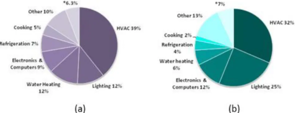
Figure 12- Total energy end use comparison between residential (a) and commercial (b) buildings, in 2006. (*) represents an adjustment factor used by IEA to reconcile two data bases. Source: [42]. ... 11

Figure 13- Simplified view of a building's heat gains and losses. ... 12

Figure 14- Dymola architecture. Source: [50]. ... 14

Figure 15- Display of a heat flow sensor model in four different layers in Modelica. ... 15

Figure 16- DES model digram implementation in Modelica. ... 16

Figure 17- Structure of Annex 60. Source: IEA EBC. ... 17

Figure 18- Neighborhood case-study layout. In some semi-detached dwellings (S1’ and S2’) the side facades were switched due to windows that were on the facades that are adjacent to other buildings. 18 Figure 19- Blueprint of ground and 1st floors (left) and physical module (right), detached dwelling (a). Blueprint of ground, 1st and 2nd floors (left) and physical module (right), terraced dwelling (b). ... 19

Figure 20- Model structure in Modelica. Bottom layer (left) and top layer (right). Dark blue lines refer to controls (internal gains and shading control), light blue to fluids (infiltration), red lines to heat transfer (W) and yellow lines to weather related data ... 21

Figure 21- Rooms.MixedAir model, from the Buildings Library. Icon layer view (a). Diagram layer schematic view (b). Source: [57]. ... 22

Figure 22- Thermal zones using the Rooms.mixedAir model. Comparison between less detailed (left) and more detailed (right) levels. ... 23

Figure 23- Heating/Cooling demand component in residential buildings (left) and in the office building (right). ... 23 Figure 24- Implementation of the internal gains released from people used in the more detailed case

Figure 25- Implementation of the internal gains released from people, used in the reference case. ... 25 Figure 26- Implementation of an automatic blinds system for shading control. ... 25 Figure 27- Comparison between Kasuda ground temperature model (red), assuming 1m depth and its annual mean value (blue). ... 26 Figure 28- Comparison of the annual heating demand per building, in MWh between case a) and b). 27 Figure 29- Comparison of the annual district heating load, in kW between case a) and b). ... 27 Figure 30- Comparison of the neighborhood’s annual heating and cooling demand between the cases considered. ... 28

Index of Tables

Table 1 – Comparison of lifecycle CO2 emissions. Emissions associated with exploration, extraction,

transportation and processing activities are taken into account. Source: [35]. ... 8

Table 2- Physical environmental and artificial design parameters that affect thermal energy requirements in buildings. ... 13

Table 3- Construction elements of the buildings. ... 19

Table 4 - 1st simulation set assumptions. ... 20

Table 5 - 2nd simulation set assumptions. ... 20

1. Introduction

Buildings in the EU are responsible for 36% of the CO2 emissions and 40% of the final energy

consumption [1] (European Commission, 2012) most of which is used for space heating. Natural gas is the main heating source, while DH systems provide 13% of the heat supply [2] (David Connolly et al., 2014). Furthermore, almost 50% of EU’s primary energy supply is lost before reaching the end use, mainly due to heat losses in electricity production [3] (David Connolly, Nielsen, & Persson, 2013), mainly through co-generation [4] (Iea, 2014). If more DH networks are implemented, some of these losses can be recycled and re-used to heating buildings, improving the overall energy efficiency of the system. In addition, 57% of EU’s population live in regions with at least one DH system, suggesting that a much higher share of DH could be used to meet the buildings’ heating needs [5] (David Connolly, Mathiesen, & Østergaard, 2012)While it is recognized that renewable heating and cooling (also through DH systems) is vital to decarburization [6] (European Climate Foundation, 2010), studies also conclude that a 50% share of DH in EU by 2050 would reduce fuel consumption by 40%, since it would replace a big share of coal, oil and natural gas used by individual boilers [3] (David Connolly et al., 2013). When sizing DH systems, one of the most important aspects to take into account is the heating and cooling needs of its users, since they will determine the amount of energy that the system will have to provide and when. To address this issue, BES tools are often used, as they can process the dynamic and complex interactions between the building’s systems in a time-efficient way especially in larger scale systems [7] (Hong, Chou, & Bong, 2000). Furthermore, these tools can be applied in the design-phase, in order to determine which options are more attractive in terms of construction materials, design and HVAC system, but also during operation and maintenance (e.g in order to identify possible failures in the building system).

However, when modelling the thermal behaviour of larger scale building systems, many assumptions need to be made in order to simplify and abstract from the complexity of reality. In that sense, and motivated by Annex 60 (subtask 2.2) this study compares and analysis how different assumptions influence the annual demand of a neighbourhood case study. More specifically, this paper focuses on the implementation of a district heating/cooling demand system using Modelica/Dymola and quantifies the difference in the annual demand in the form of a sensitivity analysis regarding the following aspects: number of thermal zones per building; ground temperature; internal gains and surroundings (the buildings are considered to be isolated, or connected to each other).

2. District Heating and Cooling

The fundamental idea behind district heating and cooling (DHC) is to connect one or more thermal energy plants to various places of consumption. The energy production is centralized and distributed through an underground piping network via steam, hot water or chilled water and transferred to buildings for use in space heating/cooling, process heating/cooling and/or hot water generation [8]. By replacing less efficient equipment in individual buildings with more efficient central production units, not only is the global energy system’s efficiency increased but also the maintenance and operation are made easier and cheaper, as the associated costs are distributed among the consumers. DHC systems make use of local fuel or heat resources and are adaptable to a large variety energy sources, providing stable and competitive energy prices and decreasing dependency on scarce or imported fuels [9]. This fuel flexibility may include both fossil fuels and/or renewable energy sources, such as geothermal heat, solar thermal and biomass. Furthermore, the ability to recover waste heat produced in industrial processes, municipal waste incineration and electricity generation processes (through CHP), composes a major advantage on energy systems and air pollution, as it provides an efficient way to reduce fossil fuels use and consequent GHG emissions. The energy supply composition of DH systems in Europe is provided in Figure 1.

Figure 1- Composition of DH in Europe, by energy source. Source: [10].

These systems are already implemented in many countries. As shown in the chart below, the European average of citizens’ percentage served by DH networks is 12.4%, with increased share in northern and eastern countries.

Figure 2-Percentage share of citizens served by DH. Source: [10].

: Recycled heat – surplus heat from electricity production, waste-to-energy plants and industrial processes. Includes two-thirds of energy delivered by heat pumps.

: Direct use of renewables in heat-only boilers and installations other than CHP. : Other – heat-only boilers, electricity and on-third of heat originating from heat pumps.

A project developed by Euroheat & Power and supported by the European Commission, named Ecoheatcool (2005-2006), analyses the heating and cooling demands in Europe in order to provide comprehensive information about these markets, as well as recommendations to encourage the development of sustainable heat and cold supply options. Figure 3 compares the DH market sales between 2007 and 2011, suggesting that there is a tendency to increase.

Figure 3- Heat Sales in DH Markets in 2007 (green) and 2011 (red), in M€. Source: [10].

Furthermore, it should be noticed that the majority of these sales occur in the residential sector, followed by the services and lastly by the industrial sector [11]. In the industrial sector, the metal, chemical, non-metallic mineral, food and paper industries are the most heat demanding ones, as they operate on high temperature levels (over 400 ºC). However, the industrial energy supply is still dominated by electricity and natural gas, while district heat represents only a minor market share [12]. In the other sectors, heat demands occur in space and water heating in residential, public and commercial buildings. The end use of net heat percentages in EU15 during 2003, by sector, are available in Figure 4.

Figure 4- End use net heat in PJ in EU15 in 2003. Source: [11]

Regarding District Cooling (DC), it should be taken into consideration that domestic air conditioning for cooling is not as common as heating. This is because it’s not as essential for comfort in residential buildings. For that matter, this sector is less supplied by DC than by DH. In addition, the residential sector may require cooling only in specific times of the year and even then the load may not be high enough to make DC economically worthy. The service sector, on the other hand, requires constant cooling for electronic equipment operation and to keep the temperature in a thermal band that increases human productivity [13]. Furthermore, service sector buildings tend to be located in areas that are close to each other, which translates into a denser load that is economically attractive. In fact, it has been shown that the electricity demand increase in many European countries over the last decades is, among other reasons, related to the required energy to run refrigerating machines, especially in the summer

6530 PJ

7100 PJ 2261 PJ

626 PJ

Net heat demand by sector

peaks [14]. This shows that the production of cooling increases the electricity demand, which means that with increasing cooling demand these peaks will be even higher and this may cause problems in the electricity grids. Although some DC technologies also run on electricity, their demand per unit cooling is lower than local cooling technologies, therefore being capable of reducing electricity demand in summer peaks. All in all, DC provides an alternative way to improve the energy systems in terms of environmental impact and energy supply, while creating business opportunities in the energy sector and its users.

Apart from a few countries, the expansion of DC in Europe during the last years is hardly significant, with a constant supply of around 3 TWh (1% of the total cooling market). The specific (per capita) DC supply market distribution in Europe is shown in Figure 5. France and Sweden (more specifically Paris and Stockholm) represent 60% of the EU27 DC market, indicating that there is a high potential for growth. However, some barriers to this growth can be identified:

 Lack of knowledge regarding general costs, environmental savings and the fact that cooling demand is increasing;

 Priority is given to modernize implemented systems, such as DH in order to reduce losses and make this technology more competitive;

 Lack of distinction between electricity consumption for cooling and for different needs;  Lack of willingness to invest in long-term return infrastructures, since emphasis is put on

low-energy prices and DC requires high investment in an initial phase.

Figure 5- European DC market in kWh/capita, in 2011. Source: [15].

A market prognosis on the cooling consumption in Europe in 2020,2030 and 2050 was performed by The European Technology Platform on Renewable Heating and Cooling, and the results are shown in

Figure 6. The significant growth between 2006/2007 and 2020 is based on an increase in the floor area.

After 2020, it is expected that technology development and social behavior will be mature enough to stop the cooling consumption increase.

In terms of potential, DHC is considered to be a key method to achieve ambitious GHG emission targets and reduce energy consumption. To demonstrate this, Euroheat & Power developed a study named Heat Roadmap Europe 2050, where the importance of having local supply and demand in urban environments is underlined. In this report, a scenario by 2030 and 2050 is drawn and compared against the one drawn in the Energy Roadmap 2050. While obtaining similar results in terms of primary energy supply and carbon dioxide emissions, the first one claims to enable a more diverse energy supply system, which is possible due to a large expansion of DHC [2].

DHC system can be classified according to heat transfer fluid (low pressure steam, hot water or hot air); thermal energy transported (heating, cooling or both); type of heat resources (separate source or recycled heat) and energy source [16]. These authors further divide a DHC system in three subsystems, consisting of a thermal energy source, thermal transportation and distribution and end consumers. These components are described in more detail in the sub-sections below.

2.1 Heating Sources

As already mentioned above, DH systems benefit from a wide range of fuel flexibility, depending on the local resources and national fuel prices and regulations. Furthermore, in larger systems where more than one energy plant is used, a priority regime regarding the heating sources hast to be established in order to guarantee that the system operation is as efficient (energetically and economically) as possible. As such, CHP plants and waste as fuel are generally used during base load periods, whereas more expensive heating sources based on fossil fuels (e.g heat only boilers) are most commonly available as stand-by peak load providers [8].

In the following sub-sections, a brief overview regarding heating technologies associated to DH systems is provided.

2.1.1 Combined Heat and Power (CHP)

Combined heat and power, also called cogeneration, refers to heat generation as a byproduct of electricity production, which would otherwise be rejected or wasted. The recovered heat increases the energy efficiency of the plant and can be made useful for heating or industrial processes, composing a major attraction when designing DH systems. In fact, when compared to conventional, separate production of heat (gas boiler) and power (gas power plant), overall energy and carbon savings of cogeneration can reach 21% [17].

CHP plants consist of four basic components [17]: The prime mover (generally a steam turbine, gas turbine or both, called combined cycle in the latter case) converts chemical energy released in the fuel combustion to mechanical energy, which is used to spin an electricity generator. The heat exhausted by these two components is recovered through heat exchangers and transferred to a boiler to raise steam at higher temperature, allowing the rejected heat to go through the distribution pipes and still be used for heating purposes by the end consumer.

As already mentioned, when combined to DH, CHP composes a major attraction, since it is able to provide thermal and electrical energy to various consumers in built environments with high, concentrated heat demand [18]. In fact, CHP-DH is already widely used in Europe, where Iceland, Finland, Sweden and Denmark hold the highest shares to satisfy their heat demands [12]. Altogether, CHP is responsible for almost 50% of the DH production in EU27.

2.1.2 Industrial Waste Heat and Waste Incineration

Industries like cement, iron and steel, glassmaking and refineries require high temperature heat to process their products, which at some point will need to be cooled down. Although efforts are aimed into increasing plants’ efficiencies by reducing the amount of heat they release, it is believed that a more cost efficient choice would be to re-use it via DH systems [13], while creating business opportunities for those industries. By doing so, not only GHG emissions would be reduced, but also large amounts of water would be saved, as it could be used for other heating purposes after the cooling process [19].

Another technology that brings environmental and energetic advantages when associated with DHS is the use of waste incineration. Waste management is currently a major priority in the EU and efforts are aimed into not only reduce waste production but also increase waste recovery, which includes re-using for electricity generation or heating purposes. This is done in waste-to-energy (WTE) plants, which collect municipal solid waste (MSW) streams and burn them in combustion chambers. MSW includes renewable energy sources, such as wood or food and non-renewable ones, such as plastics and glass. This process generates heat, which is used to boil water and produce steam that can be directly used in heating systems or to produce electricity via a turbine generator. Ultimately, this can also be seen as a good alternative to landfill disposals, which also composes a main issue within the EU. More information on combustion of MSW for DH is available in [20].

WTE plants are already widely used in Europe, where major contribution to district heat generation can for example be found in Denmark, Sweden, Finland and Switzerland [21]. Regarding industrial surplus heat recovery, however, only few applications can be found in Europe (e.g Denmark and Sweden).

2.1.3 Renewable Thermal Energy

As conventional energy sources such as oil and coal scarce and awareness regarding their effects on the environment and public health increases, many countries around the world are committing to low-carbon economies. An example is the climate and energy package, a set of targets promoted by EU leaders in order to reduce their economies’ effect on the climate by reducing energy consumption and improving energy systems. One of the three key objectives of this package, also known as the “20-20-20” is to raise the share of energy consumption produced from renewable sources by 20%, by 2020. This, together with the benefits of making use of local energy sources, makes renewable energy systems (such as geothermal heat, solar thermal and biomass) in association with DHS an essential path to achieving those targets. The role of DHS in futures renewable energy systems is discussed in [22], which concludes that the best solution towards a 100% renewable scenario by 2060 would be to continue expanding DH networks to more buildings and use individual heat pumps in the remaining ones.

As shown in Figure 1, direct use of RES in DHS is already present in many Countries in Europe, and this share is increasing [11]. The most used technologies are described below.

2.1.3.1 Geothermal

Geothermal technologies make use thermal energy stored in underground rocks and trapped liquids or vapour in order to generate electricity, heating and/or cooling. Modern technology designs include two wells (production and injection) connected to a geothermal heat exchanger. Smaller applications, such as individual space heating and domestic hot water supply can make use of a ground source heat pump, which operates on relatively low temperatures (more common at few meter depths) [23]. Furthermore, given to its immunity to seasonal variations (mostly at higher depths), geothermal is typically used to provide base-load generation.

Regarding its current application, geothermal heat is reported to contribute to 212 district heating systems in Europe [24]. A distribution of thermal energy generated from direct utilization, by category, is provided in [25]. These authors state that 12.24% of the geothermal energy used worldwide (78 countries) in 2009 were for district heating. However, when compared to its potential this technology is considered to be underdeveloped and for that matter an ongoing project called GEO-DH is being carried out by the European Commission, aiming to “accelerate the uptake of geothermal district heating” [26]. An analysis based on energy and exergy performances of three existing geothermal DHS in Turkey can be found in [27], where several suggestions on how to improve these systems’ efficiencies are presented.

2.1.3.2 Solar Thermal

Another renewable source that can easily be integrated with DHS is solar energy. Solar district heating (SDH) plants are based on solar thermal technology, which uses solar collectors to produce hot steam

distributed (solar systems is installed in a suitable location and connected directly to the DH distribution network, providing only minor contribution to the total heating load) [28]. A review of solar thermal technologies is provided by [29].

Large scale solar heating has proved to be successful when integrated with DHS, showing high reliability while requiring low maintenance [30]. In Germany, a governmental project called Solarthermie-2000 was developed in order to support the implementation of solar and seasonal storage concepts. A scope into the programme is available in [31]. Between 1996 and 2008, 11 central solar heating plants with seasonal heat storage (CSHPSS) comprising four different thermal stores and aiming to assist DH were implemented and monitored. Amongst other conclusions, authors in [32] state that within the time period, an average of 62% solar heat delivered from the collectors was supplied to the DH network. Major solar thermal assisted district heating systems can also be found in Denmark (Figure 7) and Sweden [21].

Figure 7- Large scale solar DH plants in Denmark in 2010. Source: [28]

Solar DH guidelines are provided by the European Commission, as part of a project named

SDHtake-off, which aimed to prepare a commercial market for solar thermal in new and existing DHS [33]. This

project ended in 2012 with the implementation of 180 MWth new plant capacity.

2.1.3.3 Biomass

The use of biomass and biogas for heating purposes is commonly used in Europe [21], either through CHP or heat-only boilers. As can be seen in Table 1 compared to conventional fuels, biomass releases only a fraction of CO2 in order to produce the same amount of energy, hence being considered an

essential resource to help reduce overall CO2 emission levels and meet the desired targets. In addition,

despite the increased financial cost for transporting solid biomass and physical combustion requirements, in comparison to oil or gas [34], operational costs are generally lower, which results in annual savings that over time tend to compensate initial increased investments. Also, many biomass resources are sent to landfill as waste, which in order to be disposed have associated costs. By using some of this resources as fuels, financial benefits are brought. As with other RES, biomass can bring security in terms of energy supply, as it is less vulnerable to geopolitical instabilities that result from oil and gas producing regions.

Table 1 – Comparison of lifecycle CO2 emissions. Emissions associated with exploration,

extraction, transportation and processing activities are taken into account. Source: [35].

Space Heating kg CO2/MWh

Biomass (woodchip) 10-23

Natural gas 263-302

Oil 338-369

Regarding its use in the heating sector, although natural gas is currently the main fuel in CHP plants in Europe, biomass and waste shares are increasing, having reached a 10% market share in Europe in 2012 [11]. In fact, the potential for biomass use in Europe is considerably higher than its present use, suggesting that a much higher share is possible. The use of biomass in CHP plants associated to DH in Europe was assessed by the OPET (Organizations for the Promotion of Energy Technologies), an initiative of the European Commission, in 2004 and the report is available online. It was concluded that several European countries already had a significant biomass share applied to CHP/DH (e.g Sweden, Austria and Finland) and main barriers to further implementation were identified, namely the customers’ unwillingness to pay more for green energy (in comparison with competitive fuel prices) and the lack of public environmental awareness.

A complete assessment on the European biomass potential for DH applications, by country, in terms of availability, market penetration and financing was developed by Cross Border Bioenergy, a co-foundation by the intelligent Energy Europe Programme of the European Union and is available under the name EU Handbook – District Heating Markets.

For more information on biomass use for heating, including technical and practical guides, as well as technology overviews and case studies, the following links are suggested: [36] and [37].

2.2 Cooling Sources

DCS produce chilled water, or brine, which is distributed through the piping network and absorb heat where lower temperatures are being required. The heated medium than returns to the cooling plant and is cooled again, generating a loop system. As with DH, DC can use different technologies depending on local energy prices and resource availability.

2.2.1 Compression Chillers

Compressor chillers use electricity driven motors to heat a gas by compressing it. This heat is rejected through a fan coil unit, condensing the gas into liquid [13]. After being pumped into a cooling fan coil unit, it absorbs latent heat in the air and evaporates, cooling it. Depending on the medium (water or air), the coefficient of performance (COP) can vary between 4 and 3, respectively. The COP for cooling is defined as the ratio of cooling provided to electricity consumed by the motor.

2.2.2 Absorption Chillers

In absorption chillers, heat is used as primary energy rather than electricity. As the refrigerant extracts heat from its surroundings it evaporates. The refrigerant is then absorbed into another liquid, enabling more liquid to evaporate. Using surplus heat (from industrial processes, municipal waste or even a DHS), the refrigerant evaporates and is condensed through a heat exchanger, which rejects heat at low temperature to refill the supply of liquid refrigerant and the cycle repeats itself. Although these systems hold the advantage of utilizing waste heat, the COP is lower compared to electrically driven ones. This is because the utilized heat comes generally at low temperatures, such as the ones used in DHS, decreasing the cooling capacity. Furthermore, with low heat demand during the summer, absorption chillers allow the production of cooling to increase a DHS efficiency, by the excess heat [14].

2.2.3 Free Cooling

Free cooling systems are based on available cold water reservoirs (lakes, aquifers, rivers or sea). The cold is transferred to the distribution network via heat exchangers and delivered to buildings close to the cooling plant. Examples of DCS using free cooling can be found for example in Copenhagen (Denmark) and Helsinki (Finland). In 2013, the Helsinki DCS produced 169 GWh, through different technologies as show in Figure 8.

Figure 8- Production percentage by technology in Helsinki. Source: [38].

2.2.4 Technology Comparison – CO

and PRF

In order to compare the impacts that the mentioned technologies have on the environment with conventional heating / cooling technologies, a parameter is introduced: the primary resource factor (PRF) is defined as the ratio between fossil energy supply and energy used in a building during one year for heating and cooling. In systems where only renewable energy is produced, the PRF equals zero, meaning that from production to delivery no fossil fuels are being used. Consequently, higher PRF values suggest that more CO2 is being emitted to the environment in order to deliver the same amount

of thermal energy. This parameter is useful, as it presents the advantages of DHC in a more visible way [39]. Figure 9 compares DH (a) and DC (b) with other heating and cooling technologies, in terms of PRF.

Figure 9- PRF comparison in terms of technology/resource used for heating (a) and cooling (b). Source: Euroheat & Power.

The reason for the high value defined for electricity (PRF=2.5) is because extra electricity demand is mostly met by fossil fuels, since these provide lower costs for marginal production. This value however represents the European average.

From Figure 9 it becomes clear that DH or DC use significantly less fossil energy from extraction, when present, to supply. As mentioned, higher PRF is often related to higher CO2 emissions. This is shown in Figure 10, which compares decentralized, building specific systems with centralized DHS (a) and DCS

(b) in some European cities.

Figure 10- CO2 emission and PRF for different heating (a, in g/kWh) and cooling (b, in t/MWh).

Source: [39].

2.3 Distribution

Heat from thermal plants is distributed through a piping network, delivered to the end consumers and then transported back through return pipes. According to the District Heating and Cooling Connection Handbook, develop by IEA, the sizing of the distribution pipes is ruled by four key factors: the temperature differential between supply and return, the maximum allowable flow velocity, the distribution network pressure at design load conditions and the minimum pressure differential requirements to reach the most remote consumer. Larger temperature differential allows for smaller sizes or for reduced flow velocity, which leads to decreased pumping requirements and improved system efficiency.

Regarding the heat losses, it is estimated that one tenth of the annually produced heat is lost in the network [40], caused mainly by four parameters: amount of pipe-insulation, pipe dimension (diameter and length), supply and return temperature and geographical distribution of heat demand. A method for evaluation and determination of losses in the distribution network is provided in [40]. Authors in [41] present and energy equation for a control volume in pipe, including the horizontal temperature distribution along the pipe length.

The trench length of DH pipeline systems by country is provided by Euroheat & Power, comparing 2011 with 2007 statistic as illustrated in Figure 11 and showing that overall there has been an increase, either due to expansion of existing DHS or implementation of new ones.

3. Energy in Buildings

Buildings in all sectors require energy for various purposes: in both residential and commercial buildings, energy consumption is dominated by three two purposes, namely space heating, cooling and air conditioning (HVAC) and lighting [42]. This is illustrated in Figure 12, where end use energy consumption in residential buildings is compared against commercial ones.

Figure 12- Total energy end use comparison between residential (a) and commercial (b) buildings, in 2006. (*) represents an adjustment factor used by IEA to reconcile two data bases. Source: [42].

In light of the acknowledged necessity to stop global warming by reducing energy consumption and GHG emissions, efforts are being put into reducing the energy consumption in buildings, which have been increasing due to population growth, more specific and energy consuming comfort levels and higher amount of time spent inside buildings. However, in order to act one must first understand the thermo-physical phenomena that affect this consumption. Since this study is focused on heating and cooling only, energy consumption for electric appliances will not be further addressed. As instead, emphasis will be put on processes that influence the need for HVAC.

3.1 Heat Balance in Buildings

The heat balance inside a building can be defined using the rate of heat that enters (gains) and that leaves (losses) the building over time, as presented in the equation bellow.

𝑄𝑔𝑎𝑖𝑛𝑠 = 𝑄𝑙𝑜𝑠𝑠𝑒𝑠 (1)

Within gains, two sub-categories can be identified: external and internal. External gains exist due to solar radiation through glazed constructions and are influenced by the material transmissivity. Internal gains occur due to the presence of people and electrical equipment, such as computers or washing machines and lighting. The rate of heat generated by the human body depends on the current level of activity, humidity and ambient temperature and is transferred mostly through convection and radiation, however as the ambient temperature increases evaporation becomes more relevant [43].

Regarding heat losses, four main processes can be identified: transmission losses through opaque and transparent building elements or multilayer constructions (by convection and conduction), filtration losses, which are related to the air tightness of a building, ventilation losses due to mechanical ventilation (windows, chimneys, etc) and stored heat in the building mass (which can also count as a heat gain, depending on the temperature gradient). Transmission losses occur through three different components:

 Planar building elements, such as walls, doors, internal floors, windows, etc.,  Thermal bridges,

 Ground loss through ground-coupled building elements, such as cave walls and floors.

Heat conduction and convection through planar elements is calculated assuming steady-state conditions, meaning that the heat flux is considered constant through the boundaries and layers, as bellow.

𝑞 [𝑊

𝑚2] = ℎ𝑖𝑛𝑡(𝑇𝑖𝑛𝑡− 𝑇1) = 𝑈1(𝑇1− 𝑇2) = 𝑈2(𝑇2− 𝑇3) = ℎ𝑒𝑥𝑡(𝑇3− 𝑇𝑒𝑥𝑡) (2) Eq. 2 determines de heat flux through a two-layer wall, where hint represents the interior air convection

coefficient (in W/m2_{K), T}

int the ambient temperature inside the room (in K), T1 the internal surface

temperature, T2 the temperature of the surface where the two layers connect, U1 and U2 the thermal

transmittance of the materials (in W/m2_{K) that compose layer one and two, respectively, T}

3 the external

surface temperature, hext the external air convection coefficient and Text the outside temperature. The

U-value of a multi-layered wall can be determined using the air convection coefficients (internal and external) and the thermal conductivity of the materials that compose it, using the expression below.

𝑈 [ 𝑊 𝑚2 _𝐾] = 1 1 ℎ𝑖𝑛𝑡+ ∑ 𝑥𝑙𝑎𝑦𝑒𝑟 𝑘𝑙𝑎𝑦𝑒𝑟+ 1 ℎ𝑒𝑥𝑡 𝑛 𝑙𝑎𝑦𝑒𝑟=1 (3) The thermal conductivities are expressed by k (in W/m) and x represents the length of each layer in the heat flow direction (in m). Combining Eq. 2 and Eq.3, the amount of heat that is transferred through a planar element can be determined as follows:

𝑄[𝑊] = 𝑈 ∙ 𝐴 ∙ ∆𝑇 (4)

A represents the wall are (in m2_{) that is perpendicular to the heat flow direction and ΔT the temperature}

gradient between interior and exterior air temperatures.

The heat loss through a thermal bridge assumes a higher rate than through a planar surface, which may result from a thermal conductivity higher than the one of surrounding materials or gaps in the insulation material. Because of their complexity in terms of calculation, thermal bridge losses are often calculated using computer simulation tools. The same happens with ground losses, as they are dependent on the surface’s depth, as well as on the thermal resistance of the multi-layer constructions.

Filtration and ventilation losses occur when heated air leaves the room and more heat is required to compensate the thermal loss. The amount of heat need to reach the desired air temperature depends therefore on the amount of air that left the room and on the temperature on the air brought from the outside, as shown below.

𝑄[𝑊] = 𝑐 ∙ 𝜌 ∙𝐴𝐶𝐻 ∙ 𝑉

3600 ∙ ∆𝑇 (5)

The term air changes per hour (ACH) measure how many times the air inside a volume is replaced. The specific heat of the air is represented by c (in KJ/Kg K) and the air density by ρ (in kg/m3_).

The processes that influence the heat balance between a building and the exterior are illustrated in

Figure 13.

Figure 13- Simplified view of a building's heat gains and losses.

All in all, there are many parameters that influence a building heating and cooling requirements. These parameters are listed in [44], as shown in Table 2- Physical environmental and artificial design

Table 2- Physical environmental and artificial design parameters that affect thermal energy requirements in buildings.

Physical environmental parameters Artificial design parameters

Hourly outdoor temperature (ºC) Building form factor Transparency ratio

Solar radiation (W/m2) Orientation

Thermo-physical properties of building materials.

Wind direction and velocity (m/s) The distance between buildings

Using these parameters, an overview of building design criteria that can reduce thermal energy demand in residential buildings is provided in [45].

Furthermore, there are many ways to predict the thermal behavior of buildings. A review on such methods, including the use of building performance simulation (BPS) tools is available in [46].

3.2 Building Performance Simulation (BPS)

The physical environment on which a building is set is constantly in motion. Analytical approaches for energy calculations are possible in steady-state and simplified conditions, when all variables are known. However, when calculating the energy flows over time and taking into consideration more realistic processes, the number of equations required and the complexity of the system increases significantly. For this matter, BPS tools are often used by companies and researchers, which provide them with solving procedures at a computational speed level, allowing them to focus more on the physical processes than on their mathematical expressions. Computational BPS has been widely and successfully used to evaluate design alternatives in the design phase of new buildings and in retrofit measures of existing ones, demonstrate code compliance and calculate performance ratings [47]. More recently, these tools are being used to predict energy performance of buildings. The energy performance of a building is driven by six key factors: climate, building envelope, building equipment, operation and maintenance, occupant behavior and indoor environmental conditions (IEA Annex 53: Total energy use in buildings: Analysis and evaluation). With BPS tools it is possible to integrate all these factors in order to understand how each one affects the performance of buildings and under which conditions, composing an important step to improve design and operation of building systems with reduced energy consumption [47]. Depending on the purpose, different BPS tools can be used. An overview of twenty widely used programs over the last decades (including EnergyPlus, ESP-r, IDA ICE and TRNSYS) is provided in [48] and a comparison is drawn in terms of many relevant categories, such as zone loads, building envelope, renewable energy systems, HVAC systems, environmental emissions, etc. Among many conclusions, it was noticed that in some cases relying on a single simulation tool isn’t as productive as using different tools in different work stages. This clearly shows the necessity of computer-based simulation environments that are able to receive inputs from different BPS tools and integrate them as a single model. Such a software is described in the following section.

4. Dymola/Modelica

Dymola (Dynamic Modeling Laboratory) is a simulation environment developed by Dessault Systèms AB with the purpose to provide a wide range of physical systems modeling. Based on modern methodologies using object orientation and equations, it supports hierarchical model composition, containing libraries of reusable components, connectors and composite acausal connections. Acausal modeling means that more emphasis is put on the physical relations between the models, using Differential Algebraic Equations (DAE), rather than on the mathematical complexity based on Ordinary Differential Equations (ODE) used in causal modeling. While causal models take into account computational order, this isn’t considered in acausal modeling [49].

The architecture of Dymola is shown in Figure 14. Furthermore, this simulation tool contains a symbolic translator for Modelica equations generating C-code for simulation, which can be extracted and imported to MATLAB-Simulink and hardware in-the-loop platforms.

Figure 14- Dymola architecture. Source: [50].

Modelica is a freely available object-oriented modeling language developed by the Modelica Association to approach large, complex and heterogeneous physical systems [50]. Modelica comes with Modelica Standard Library (MSL), a constantly upgraded package including the following features:

 Blocks (library of basic input/output control blocks),

 ComplexBlocks (library of basic input/output control blocks with complex systems),  Constants (library of mathematical constants and constants of nature),

 Electrical (library of electrical models),

 Fluid (library of 1-dim thermos-fluid flow models),  Magnetic (library of magnetic models)

 Math (library of mathematical functions and of functions operating on vectors and matrices),  Mechanics (library of 1-dim and 3-dim mechanical components),

 Media (library of media property models),

 SIunits (library of type and unit definitions based on SI units according to ISO 31-1992),  StateGraph (library of hierarchical state machine components to model discrete event and

reactive systems),

 Utilities (library of utility functions dedicated to scripting).

All these features include classes that are prepared for direct application, each being categorized by four different layers. Figure 15 shows a class from the Thermal package that represents a heat flow sensor between two ports. In the Icon layer (a) displays the class in an external way, almost as a physical representation of the sensor. In the Diagram layer (b), the objects that characterize the class are present and connected to each other, creating the modeling environment in a graphical way, while the Modelica Text layer (c) holds these in an equation text-based form. Finally, the Documentation layer (d) provides the user with valuable information about the class.

Figure 15- Display of a heat flow sensor model in four different layers in Modelica.

4.1 Applications

Being suited for multi-domain modeling, Modelica is used for various applications, such as mechatronic models in robotics, automotive and aerospace sectors involving mechanical, electrical, hydraulic and control subsystems [51].

More recently, Modelica is being used in energy systems-related applications, such as building performance simulation (BPS) and energy grids testing incorporating various sources of supply. In the context of district energy systems, several studies have been developed using Modelica: the influence of reducing the district demand on the mass flow rate of the district network branch is discussed in [52], while [53] presents a methodology for simulating large-scale energy systems, namely a district supplied by a CHP-DHS. Figure 16 shows a model diagram for a District Energy System (DES) presented in [54] fed by electrical energy, hot water and natural/bio gas flows including both fossil and renewable generation.

Figure 16- DES model digram implementation in Modelica.

4.2 Buildings Library

In order to approach building energy and control systems, an open-source library was developed by the Lawrence Berkeley National Laboratory (LBNL) of the United States Department of Energy [55]. The Buildings Library meets the needs for simulation-based innovation in building systems, providing support for rapid prototyping, modeling of arbitrary heating, ventilation and air-conditioning (HVAC) system topologies, development, verification and hardware-in-the-loop testing of control algorithms, stabilization of feedback control and emulation of faults at the whole building-system level [56]. All in all, the library provides users with a collection of models that can be used, extended and adjusted to meet individual needs. The following main packages are included [57].

 Airflow: Holds models that compute airflow between the interior and exterior environment, using pressure differences as driving force.

 BoundaryConditions: Contains models that read and compute boundary conditions such as weather related data.

 Controls: Contains blocks that model continuous and discrete time controllers and blocks that can be used for schedules and set points.

 Fluid: Contains component models for air- and water-based HVAC systems, such as chillers, heat exchangers, pumps, energy storage, etc.

 HeatTransfer: Holds models for steady-state and dynamic heat transfer through opaque constructions and glazing systems.

 Rooms: Contains models for heat transfer in rooms and through the building envelope.

 Utilities: Several utilities, such as computing thermal comfort and psychometric functions are available in this package.

Furthermore, the developed models have been validated using different methods [56]: window heat transfer and transmitted solar radiation was tested against measure data (empirical testing), optical properties and surface temperature of windows were compared with other simulators (comparative testing), the building envelope model was validated using the BESTEST (ASHRAE 2007) method and individual component models such as heat and mass transfer were compared with exact solutions (analytical verification).

To conclude, the library is filled with examples that provide the users with good information on how to apply the developed methods, presenting a good way for new modelers to start using Modelica.

5. Motivation - IEA Annex 60

5.1 Overview

Recent changes in the requirements for buildings, such as the 2010 Energy Performance of Buildings Directive and the 2012 Energy Efficiency Directive of the European Commission on reducing the energy consumption, bring new challenges to BES tools, as future research will be based on the development and implementation of renewable energy generation and distribution on a community level [58].

Conventional simulation programs focus mainly on the energy analysis on an individual building level and are therefore not suited to investigate the interaction between buildings and district energy systems [59]. Furthermore, they’re integration with models from different BES tools or models created by different team members is unpractical, which also makes it difficult to analyse existing buildings with unconventional systems and control logic implementation. In addition, BES faces other challenges today that were not present when current simulation programs were developed, such as model-based design of integrated buildings by design firms, including processes based on a Building Information Model (BIM), i.e. a data model that entirely describes a building. These models shall be used not only in the design phase, but also to support operation by providing fault detection and diagnosis, as well as operation strategies for energy grid integration.

In light of the above mentioned, the International Energy Agency Energy in Buildings and Communities Programme (IEA EBC) initiated a recent project, called Annex 60. It comprises 41 institutes from 16 countries and the objectives are to develop and demonstrate next-generation computational tools ‘that

allow building and community energy grids to be designed and operated as integrated, robust, performance based systems’ [60]. To address this issue, Modelica and the Functional Mockup Interface

(FMI) standard have been selected, ‘as they are industrial-strength, non-proprietary, industry-driven

standards that allow technology transfer between the building performance simulation community and much larger dynamic modelling communities from controls, automotive, power-plant, electrical system and chemical plant modelling’ [60]. Annex 60 will be conducted through three subtasks: Subtask 1 will

validate and further develop the technology required (modelling libraries and tools for co-simulation), Subtask 2 explains and applies these technologies to a case study and finally Subtask 3 will develop a guidebook. The structure of the Subtasks is illustrated in Figure 17.

Figure 17- Structure of Annex 60. Source: IEA EBC.

This study is focused on Subtask 2 - Activity 2.2, which deals with the demonstration in Modelica of buildings’ integration into a community-level energy grid. The initial phase of this subtask consisted of a common exercise, called “Reference Annex 60 Neighbourhood Case”, which definition is available in the section bellow. Annex 60 started in 2012 and will be finished by 2017.

5.2 Subtask 2.2 – Neighbourhood case study

The case study designed by IEA’s Annex 60 consists of a 24 buildings’ neighbourhood, combining residential and commercial buildings, which are combined to describe a street section. The buildings are classified in five layout typologies: detached (D), semi-detached (S) and terraced (T) dwellings, one five storey apartment building (A) and one five storey office (O) building. Furthermore, the buildings are can have one of two insulation typologies: state #1 (more insulated) and state #2 (less insulated, more common in older buildings). These levels of insulation denote the one required by EPBD (Energy Performance of Buildings Directive) 2010 in Flanders (Belgium) (#1) and the one found on buildings of period 1946-1970 in Flanders based on the IEE (International Energy Europe) TABULA (Typology Approach for Building Stock Energy Assessment) project (#2).

Figure 18- Neighborhood case-study layout. In some semi-detached dwellings (S1’ and S2’) the side facades were switched due to windows that were on the facades that are adjacent to other buildings.

Given the considerable amount of buildings, the neighbourhood was divided into five zones, according to their orientation. The orientation is determined assuming that each building is street oriented. In addition, a piping distribution network was also provided, including the distances between the main distribution pipe and the ones connecting to the buildings, in order to take into account, the resulting heat losses. However, such losses were not considered in this study and therefore the distribution network is not included in Figure 18.

The geometry of each building, as well as construction materials and parameters were given in the exercise layout. Regarding the geometry, the provided blueprints were further drawn in AutoCAD and physical modules were made, as these provided a better view of the building structure and consequently of the whole district. The blueprints of the detached- and the terraced dwellings, as well as the corresponding physical module, are presented in Figure 19.

The residential dwellings are all characterized by one ground floor (daily-zone), one floor with bedrooms (night-zone) in the detached and semi-detached, two floors with bedrooms (night-zones) in the terraced dwelling and one unheated attic. Each floor of the apartment building has a daily- and a night-zone in opposing facades and an unheated hallway between them. Regarding the office building, it has the same geometry as the apartment but in this case the hallway belongs to the “night-zone”.

Figure 19- Blueprint of ground and 1st floors (left) and physical module (right), detached dwelling (a). Blueprint of ground, 1st and 2nd floors (left) and physical module (right), terraced dwelling (b).

The U-value of the building envelope, internal floor, doors and windows is shown in Table 3 for both insulation states.

Table 3- Construction elements of the buildings.

Construction State #1 State #2 Elements U-value [W/m2_K] Elements U-value [W/m2_K]

Facade Cavity wall with 6 cm mineral wool wall

insulation

0.4 Outer brick leaf, air cavity 5cm, inner brick leaf

1.7

Roof 10 cm mineral wool roof insulation between

rafters

0.3 Wooden roof construction with tiles, interior finishing

2.85

Floor 5 cm XPS floor insulation below screed 0.4 Concrete structural floor, floor screed

and floor finishing

3.0

Windows Insulated profiles Uframe 1.8 - high

performance glazing Uglas 1.1

1.7 Wooden window profiles - single glazing

5.0

Doors Insulated door leafs 2.9 Un-insulated door leafs 4.0

Regarding the heating needs, a constant temperature set-point for heating is defined as 21 o_{C for all}

buildings, meaning that when the inside temperature drops below this value, heat will be injected into the building. No cooling was considered in the first stage of the common exercise, nor were internal gains.

The objectives were to implement the district in Modelica and determine the annual heat demand, as well as identify the peak loads for each building and for the whole district. The general assumptions, as well as the model development are described in the following section.

6. Methodology

The simulations were carried in two different sets. The first set was used to address the common exercise of Annex 60-subtask 2.2, which considers the assumptions mentioned in the case study (see 5.2), while discharging cooling needs, internal gains and shading control. For this set, a comparison was conducted between assuming the buildings were separated from each other (a) and in contact with each other (b), exchanging heat through conduction. Both cases are summarized in Table 4.

Table 4 - 1st simulation set assumptions.

For the second set, more parameters were included: occupancy schedules, cooling needs and shading control. The objectives of developing the second simulation set were to understand how the referred parameters can be modelled in Modelica and compare how different resolution levels influence the results. As such, five cases were defined for comparison (a-e). On each case, the detail level of a specific parameter (ground temperature, internal gains, number of thermal zones and surroundings) was individually increased and compared against the reference case (a), in order to perform the sensitivity analysis. The four parameters in study were modelled in two levels of detail each. These cases are summarized in the table below.

Table 5 - 2nd simulation set assumptions.

2nd set: (a) Ref Case Comparison

Heating Tset-point for heating in residential buildings = 21 (constantly)

Tset-point for heating in office building = 20 (occupied), 16 (unoccupied)

Cooling Tset-point for cooling in office building = 24

Thermal Zones 1 per building b) day/night zones

Internal Gains Constant annual mean gains c) Variable gains based on schedules

Shading Control Shading Threshold = 300 W/m2

Ground Temperature Tground = constant d) Tground = f(depth)

Surroundings Buildings are isolated e) Buildings are connected

In the reference case, the lowest resolution level was adopted. This includes assuming each building as a single thermal zone, constant hourly internal gains, constant ground temperature and isolated buildings (not in contact with each other). In case (b), more thermal zones were assumed (day and night zones such as in the first simulation set), while in case (c) variable internal gains based on occupancy schedules were assumed. Cases (d) and (e) take into account the thermal variability of the ground and the heat exchange between the buildings, respectively.

The subsection below describes in more detail how the models were developed and implemented in Modelica and how the levels of detail applied differ from each other.

1st set: Ref. Case (a) Comparison (b)

Heating Tset-point for heating = 21 (constantly, for all buildings)

Cooling Not considered

Ground Temperature Tground = 10.3

Internal Gains Not considered

Shading Control Not considered

Thermal Zones Day/night zones

6.1 Implementation in Modelica

The model was structured in two layers. The bottom layer contains the building’s envelope related parameters, such as geometry and construction materials’ properties. As can be seen Figure 20 (left), the infiltration was also included in this layer, assuming 0.1 ACH for state #1 buildings and 0.5 ACH for state #2 ones. The heat balance inside the building is calculated here, using the model

Rooms.MixedAir from the Buildings library (described further in 6.1.1).

In the top layer, the implementation of control based components allows relevant information to be added to the building(s), e.g. regarding its occupancy schedules, shading controls and the ground temperature. This is done by connecting ports that are implemented in the bottom layer and visible in the top one, allowing a data exchange between the building structure and the parameters that influence its demand. The heating /cooling demand meter is also connected to the building in this layer. In order to evaluate how the representation of the parameters in study influences the heating/cooling needs of a building, each parameter was modelled separately as a sub-system. This provides independency between the sub-systems, guaranteeing that by changing their level of detail one does not have to alter the whole system.

Figure 20- Model structure in Modelica. Bottom layer (left) and top layer (right). Dark blue lines refer to controls (internal gains and shading control), light blue to fluids (infiltration), red lines to heat transfer

(W) and yellow lines to weather related data

In addition, it allows one sub-system to connect to any number of buildings as long as they have the same layout typology. For example, the internal gains defined for the terraced dwellings only need to be processed once, passing the information to all terraced dwellings. Not only this saves simulation time but also makes the model more user-friendly.

6.1.1 Thermal zones

Each building was defined using one (or more, depending on the case) thermal zones. In order to represent each zone, a mixed air room model from the Buildings library was used, where the constructions and surfaces that participate in the heat exchange processes were defined. These constructions are divided in exterior construction without window, exterior constructions with window,

partition constructions and constructions that expose other-side boundary conditions. The last ones are

used to connect one surface that is connected to the room heat balance and to another surface that is connected to the heat port, which is connected to different thermal conditions (used to connect the floor to the ground, or to establish heat transfer between different thermal zones). The heat conduction through the multi-layered materials is computed one-dimensionally. Their (materials) properties are defined in data records (construction parameters). The solar radiation that is absorbed by each window is computed in the model solar radiation balance and includes infrared radiation exchange, heat conduction and heat convection. The convective and radiative heat transfer to the ambient and the sky is computed in the model outside boundary conditions. The port labelled heat port, connected to air volume is used to couple a sensor for the temperature inside the room and may be used to add a sensible convective heat flow to the room air. This port was used to connect the building to the demand meter, as will be explained

in 6.1.2. The models shade control signal and internal heat gain signal allow control based data to be added to the room heat balance. A complete overview of the Rooms.MixedAir model is provided by [57].

Figure 21- Rooms.MixedAir model, from the Buildings Library. Icon layer view (a). Diagram layer schematic view (b). Source: [57].

As mentioned in 6, two levels of detail were considered regarding the number of thermal zones used to represent the buildings: The first level considers each building as one single zone (plus an unheated attic in the residential dwellings). In the second level, the single zone assumed in the first level is divided in daily- and night zones (as mentioned in 5.2). This division of the living space allows a more realistic characterization of the heat transfer inside the building, as it separates two zones that are different in terms of occupancy. An accurate sub-zoning for residential buildings in building simulation is described in [61], taking into account different thermal comfort bands for three distinctive zones: bedrooms, bath rooms and other rooms. It concludes that the adaptation to the outdoor temperature plays a major role in the thermal comfort inside the building and defines a strong dependency of the comfort bands on the recent outside temperature values. However, such sub-zoning would increase the number of

Rooms.mixedAir models needed to represent each building, which would result in an unpractical

simulation time. For the same reason, the second simulation set only considers one thermal zone per building, since it includes more simulations than the first set.