Vol.50, n. 6 : pp.1051-1060, November 2007
ISSN 1516-8913 Printed in Brazil BRAZILIAN ARCHIVES OF
BIOLOGY AND TECHNOLOGY
A N I N T E R N A T I O N A L J O U R N A L
Assesment of Soil Erosion by
137Cs Technique in Native
Forests in Londrina City, Parana, Brazil
Avacir Casanova Andrello1*, Carlos Roberto Appoloni1 and Virgílio Franco do
Nascimento Filho2
1
Departmento de Física; CCE; Universidade Estadual de Londrina; C. P.: 6001, 86051-390; Londrina - PR -
Brasil. 2Loboratóerio de Instrumentação Nuclear; Centro de Energia Nuclear em Agricultura; Universidade de São
Paulo; Av. Centenário, 303; C. P.: 96; 13400-970; Piracicaba - SP - Brasil
ABSTRACT
The aim of this work was to assess the soil erosion process in native forest by the 137Cs methodology. The mass
balance model was applied to assess the rates of soil loss in three native forests around of Londrina city, Paraná,
Brazil. 137Cs distribution depth was of exponential type for the three forests and 137Cs inventory was 241 Bq m-2 for
Mata 1, 338 Bq m-2 for Mata 2 and 325 Bq m-2 for Mata UEL. The soil loss value calculated for three native forests
was: 6,684 kg ha-1 yr-1 for Mata 1, 1,788 kg ha-1 yr-1 for Mata 2 and 4,524 kg ha-1 yr-1 for Mata UEL.
Key words: Cesium-137, mass balance model, native forest
* Author for correspondence
INTRODUCTION
Soil erosion is the foremost cause of the ecosystem degradation. Many studies have been carried out to understand this problem, but they are time consuming and expensive. Moreover, these studies were conducted in the plots that did not represent major areas adequately being applied only for the cultivated soils or undisturbed soils of pasture. In undisturbed soil forest, the hydro erosion impact depends on the type and quantity of canopy and very few studies have been dedicated to the qualitative and quantitative understanding of this. In this ecosystem, the crash drop of the rain is reduced by treetop and mold on soil surface, so that hydro erosion is reduced. However, soil redistribution in native forests can occur by other processes, such as diffusion, migration of soil particles in the soil matrix, and bioturbation and
self-evolution of forests. For these reasons, the conventional methods are limited to quantify soil redistribution, and consequently, the soil erosion rates for this environment. A conventional method is the RUSLE (Revised Universal Soil Loss Equation; Renard et al, 1991) that has been utilized in study of soil erosion for the cultivated soils or pastures, but very few were applied to undisturbed soil forests (Özhan et al, 2005; Erskine et al, 2002; Wallbrink et al, 1998).
Another method that has been applied to study the
soil erosion and deposition is the 137Cs
methodology. 137Cs is an anthropogenic
1971; Poinssot et al, 1999, Onodera et al, 1998) and its redistribution in the environment occurs by the physical processes (principally by erosion). Organic matter quantity in the superficial soil horizons determines the 137Cs availability for the
downward diffusion and migration in the soil matrix. Many papers have shown that when 137Cs
is adsorbed by the minerals parts of the soil, its desorption by the natural chemical processes does not exist or is very unready (Vlacke and Cremers, 1994; Facchinelli et al, 2001). Hence, 137Cs has become a soil marker and has been utilized in the soil erosion assessment (Andrello et al, 2003 and 2004). Several empirical and theoretical models have been proposed to soil erosion quantification (losses or gains) by 137Cs redistribution (Walling and He, 1999). To use these models, a reference inventory value for 137Cs is determined and then compared with 137Cs inventory determined for the sampled soil. If studied soil has less 137Cs than reference value, then the soil loss would occur, otherwise, soil deposition would take place. Thus, the reference 137Cs inventory is necessary to
establish a correlation between the 137Cs
redistribution and soil erosion. 137Cs depth distribution in undisturbed soil can be used to show the bioturbation occurring in the soil since
137Cs deposition by fallout. In recent years, many
papers have been devoted to study the migration of
137Cs in the soil system, but, this process is not
fully understood because it’s complex and a large number of parameters may affect the migration of
137Cs in the soil system. It is well known that
bioturbation can contribute significantly to the vertical transport of fallout radionuclides that might have a considerable impact on the long-term in the depth distribution profile of radionuclides. Bioturbation can occur due to a variety of endopedonic animals’ activity, of that the earthworms are very active in consuming and excreting large amounts of the soil. It can transport the soil components downward and upwards in the soil matrix, which can change considerably the morphological structure of the soil. Although in the grassland soils some information on the effect of bioturbation on the transport of fallout radionuclides is available, but this information is not available for the forest soils.
The aim of this work was to study the soil erosion occurring in three forests around Londrina city, Parana, Brazil and to assess the long-term bioturbation in the soil profile of these forests by
MATERIALS AND METHODS
The Model
The mass balance model developed by Kachanoski and de Jong (1984) and adapted by Yang et al. (1998) was utilized in this work. This model considers the 137Cs annual deposition through overall fallout period (1954 to early 1980s) and can be applied to determine the soil erosion rates in undisturbed soils. For any year t, the mass balance model can be represented as:
t t 1 t
t S F E
S = − + − (1)
where St is the total 137Cs inventory in the soil
profile at year t (Bq m-2), St-1 is the total 137Cs
inventory in soil profile at year t-1 (Bq m-2), F t is
the total 137Cs deposited by fallout at year t (Bq m -2), E
t is the amount of 137Cs lost of soil profile at
year t (Bq m-2), where t changes from 1 to N (N =
M – 1954, M is the sampling year). Assuming that there is a constant erosion rate, this model can be utilized to assess the total 137Cs content in the soil
at end of elapsed time. Although, assuming that the soil erosion rate is constant does not correspond to the true, it can be applied because an average soil loss will be obtained for the studied time period.
If the total amount (Ct) and annual fraction (rt) of 137Cs deposited by fallout on the region during an
elapsed time period are known, Ft can be
expressed as:
t t
t r C
F = (2)
Due to the lack of total 137Cs deposition data of
monitoring stations for the most regions of the world, the reference 137Cs inventory (CR, in Bq m -2) determined in the study area in the specific year
t can be used instead of Ct, so that Ft can be
rewrite as:
R t
t r C
F = (3)
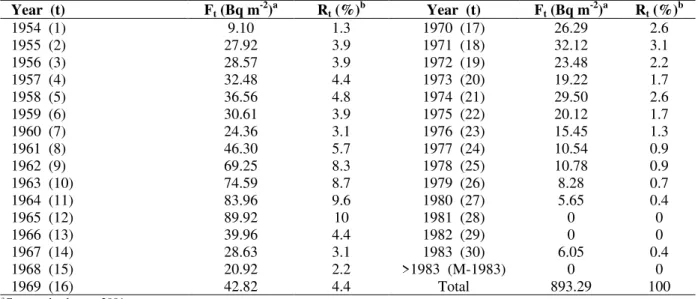
Although the reference 137Cs inventory is easily determined in the study area, the same not occur to the annual fraction (rt). However, despite of total 137Cs level deposited is different in several regions
Walling and He (1997), values of rt for South
Hemisphere were determined and was shown in Table 2, in the form Rt = 100 x rt. The contribution
due to Chernobyl accident was not considered in these values.
Study Area
In this work, the mass balance model was applied to assess the soil loss in the three native forests around Londrina city, Paraná State, Brazil. The native forests were labeled as Mata 1, Mata 2 and Mata UEL. The vegetation of these native forests is lowland rainforest and the soil belongs to the group Oxisols by U. S. soil taxonomy. The slope of Mata 1 changes from 10 to 20%, while slope of Mata 2 is lower than 1% and the slope of Mata UEL is around of 5%. Mata 1 had a 3 cm thickness of mulch on soil surface and a great quantity of little roots down to 20 cm depth. Mata UEL had approximately 2 cm thickness of mulch on soil
surface and little roots down to 5 cm depth. Mata 2 had a thickness of mulch minor than 1 cm on soil surface and almost nothing of little roots. The granulometric properties of the soil for three native forests are shown in Table 1. These values were obtained by homogenization of three cores of each native forest resulting in one sample that was analyzed to granulometric properties. This procedure was utilized because the soil of the three native forests was the same group. The studied areas are located around the coordinates of 23016’
S and 51017’ W. The mean elevation of the areas
is around 665 m above sea level. The regional climate is classified as humid sub-tropical (mean temperature = 20.7 oC) with rainfall throughout the year, with a great probability of winter dryness (Corrêa et al., 1982). The average annual rainfall
was 1615 mm yr-1, based on measurements carried
out at surrounding meteorological sites, from 1975 to 1998.
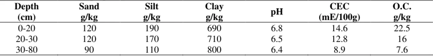
Table 1 - Granulometric properties of the soil of the three native forests.
Depth (cm)
Sand g/kg
Silt g/kg
Clay
g/kg pH
CEC (mE/100g)
O.C. g/kg
0-20 120 190 690 6.8 14.6 22.5
20-30 120 170 710 6.5 12.8 16
30-80 90 110 800 6.4 8.9 7.6
O.C. – Organic Carbon
Sampling and Analysis
In the three native forests the sampling point was chosen the farthest possible of big trees and probable holes left for dead trees, in order to avoid the possible 137Cs accumulation due to the rain
water flowed by the tree stem and root during the fallout period. In each native forest a point was sampled 1, 2, 4 and 5 cm increment at depth down to 25 cm. In order to diminish the punctual variability, each sample, with 2 kg of soil, was
obtained from three replicates sampled from 1 m2
area. The samples were air dried for 48 h, grounded for < 2 mm, and packaged in Marinelli beaker of 2 l for 137Cs activity determination. The activity determination was realized by gamma-ray spectrometry with 10 and 20% relative efficiency HPGe detector. The detection time was 216,000 s for the 10% detector and 54,000s for the 20% detector. The software MAESTRO model A65-B32, version 4.10, was utilized for the spectra analysis.
RESULTS
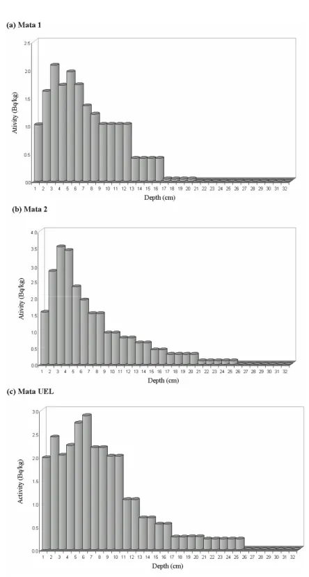
137Cs distribution profile for three native forests
was of exponential type (Fig. 1). This was in accordance with other results for the undisturbed soils (Walling and Quine, 1995). A mathematical model utilized to describe this distribution form could be given by the equation:
z
s
e
C
ba
−=
(a > 0 and b > 0) (4)where Cs is 137Cs concentration (Bq kg-1) at the
depth z (m) and a and b are the function
coefficients. The a coefficient represented the amount of 137Cs that should be there in the superficial soil if soil loss or soil redistribution did not occur. The b coefficient represents the shape of the 137Cs depth distribution profile. Hence, greater
b showed more shallow 137Cs depth distribution
profiles.
Following Yang et al (1998), if 137Cs distribution
where f(z) is a function of depth z (m), then 137Cs
concentration Cs (Bq kg-1) is:
) z ( f
Cs= (5)
Hence, the reference 137Cs inventory (C
R, in Bq m -2) can be represented as:
∫
=H 0R Df(z)dz
C (6)
where D is the soil bulk density (kg m-3) and H is
depth (in m) in which 137Cs still can be detected.
Let h be the mean annual thickness of the superficial soil loss, the mean annual 137Cs loss
(λ), relative to the total 137Cs present in the soil profile, can be determined by the expression:
∫
∫
∫
∫
− = = λ H 0 H h H 0 R h 0 dz ) z ( f D dz ) z ( f D dz ) z ( f D C dz ) z ( f D (7)in which λ may assume values between 0 and 1. The 137Cs loss in year (t) can be determined by:
t 1 t t t F S E + = λ −
(0≤λ≥1) (8)
where Et (Bq m-2) is the 137Cs lost at year t, St-1
(Bq m-2) is total 137Cs inventory at year t-1 and F t
(Bq m-2) is the amount of 137Cs deposited by
fallout at year t. In undisturbed and stable soils, it is expected that 137Cs distribution profile would be similar to several years, i.e., remain being exponential type. Rogowski and Tamura (1970) and Filipovic-Vicenkovic et al (1991) have observed this behavior during several years for the undisturbed soils. If there is no major perturbation in the soil, an exponential 137Cs distribution depth may stay year after year, hence, in first approximation it can be assumed:
= λ =
λt constant (t=1,2,...,N;0≤λ≥1) (9)
Using equation (9) in (8), we get:
) F S (
Et=λ t−1+ t (10)
Equations (10) and (3), equation (1) can be re-written as follows:
) C r S ( ) 1 (
St= −λ t−1+ t R (t=1,2,...,N)(11)
Solving this equation until t = N, it would be:
R N R 3 2 N R 2 1 N R 1 N N C r ) 1 ( ... C r ) 1 ( C r ) 1 ( C r ) 1 ( S λ − + + λ − + + λ − + λ − = − − (12)
where SN is 137Cs inventory in eroded soil profile
at sampling year.
Let 137Cs inventory at sampling year be denoted by
CE, then SN = CE. Keeping CR in equation (12), it
would be: } r ) 1 ( ... r ) 1 ( r ) 1 {( 1 C C 1 N 2 1 N 1 N R E λ − + + + λ − + λ − − = − − (13) Let 100 C C C Y R E R × −
= (14)
and 100
r
Rt= t× (15)
where Y is percentage of 137Cs loss in relation to
the reference inventory at sampling year and Rt is
the percentage fraction of total 137Cs fallout
deposition at year t.
Table 2 showed that Rt = 0 after 1983, then
equation (13) became, (for M > 1983):
1983 M 29 3 26 2 27 1 28 ) 1 ( } R .... R ) 1 ( R ) 1 ( R ) 1 {( 100 Y − λ − + + λ − + + λ − + λ − − = (16)
As the values for Rt are given in Table 2 and the
values for CR can be calculated by equation (6)
and (4), then, it is only necessary to determine the values of CE to assess the mean annual 137Cs loss
(λ) for each native forest. The values of CE for
each native forest was determined using the following equation:
∑
= × × = z 1 i i i iE C D I
C (17)
where Ci is the 137Cs activity in the i th depth (Bq
(kg m-3), I
i is the depth increment in the i th depth
(m) and z is the maximum number of depth increment until the depth where 137Cs can be
detected. The values of CE for three native forests
are presented in Table 3.
As the function f(z) that represents the 137Cs
distribution profile was known for th three native forests, it is possible to determine the reference inventory CR for each native forest through the use
of equations (4), (5) and (6) and the values for a and b. Then, it was possible to determine Y by equation (14) for each native forest. The values of CR and Y for each native forest are shown in Table
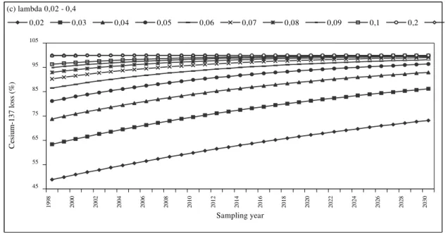
3. As possible to λ assume values from 0 to 1, it was realized several iterations with equation (16), with λ changing from 10-4 to 0.4 and M changing
from 1988 to 2030. Graphics for Y, with Y changing from 0% to 100%, was obtained from these iterations. Utilizing these graphics, values of
λ is possible to be determined, since values of Y are known, and vice-versa. With the values of Y obtained for the three native forests and with the
graphics given in Fig. 2, the λ value was calculated for each native forest, and the mean annual thickness of soil loss (h) for each native forest was determined by equation (7). The λ value and h for each native forest are shown in Table 4. Knowing h, it was possible to calculate the mean annual soil loss by the following equation:
10000 D
h
ER= × × (18)
where ER is the mean annual soil loss (kg ha -1 yr-1), h is the mean annual thickness of soil loss
(m), D is the soil bulk density (kg m-3) and 10000
is a conversion factor from hectare to square meter.
A mean soil bulk density of 1100 kg m-3 was
utilized to calculate the mean annual soil loss for the three native forests. The values for ER are
shown in Table 4.
Table 2 – Values of 137Cs annual deposition (F
t) and the 137Cs annual fraction (Rt) deposition to the South
Hemisphere (based on Walling and Quine, 1997).
Year (t) Ft (Bq m-2)a Rt (%)b Year (t) Ft (Bq m-2)a Rt (%)b
1954 (1) 9.10 1.3 1970 (17) 26.29 2.6
1955 (2) 27.92 3.9 1971 (18) 32.12 3.1
1956 (3) 28.57 3.9 1972 (19) 23.48 2.2
1957 (4) 32.48 4.4 1973 (20) 19.22 1.7
1958 (5) 36.56 4.8 1974 (21) 29.50 2.6
1959 (6) 30.61 3.9 1975 (22) 20.12 1.7
1960 (7) 24.36 3.1 1976 (23) 15.45 1.3
1961 (8) 46.30 5.7 1977 (24) 10.54 0.9
1962 (9) 69.25 8.3 1978 (25) 10.78 0.9
1963 (10) 74.59 8.7 1979 (26) 8.28 0.7
1964 (11) 83.96 9.6 1980 (27) 5.65 0.4
1965 (12) 89.92 10 1981 (28) 0 0
1966 (13) 39.96 4.4 1982 (29) 0 0
1967 (14) 28.63 3.1 1983 (30) 6.05 0.4
1968 (15) 20.92 2.2 >1983 (M-1983) 0 0
1969 (16) 42.82 4.4 Total 893.29 100
aCorrected values to 2001. bR
t = 100 x rt
Table 3 – Values of a and b coefficients, total 137Cs inventory (CE), reference inventory (CR) and percent 137Cs loss
(Y) obtained for three native forest.
a (Bq kg-1) b (m-1) CE (Bq m-2) CR (Bq m-2) Y (%)
Mata 1 3.18 10.26 240.6 296.6 18.83
Mata 2 5.09 14.48 337.6 365.4 7.61
Table 4 – Values of mean annual 137Cs loss (λ), mean annual thickness of the superficial soil loss (h) and the mean
annual soil loss (E)R for three native forest.
λ h (x10-2 m) ER (kg ha-1 yr-1)
Mata 1 0.0057 0.056 6684
Mata 2 0.0022 0.015 1788
Mata UEL 0.0035 0.038 4524
DISCUSSION
The 137Cs distribution profile for three native forests is presented in Fig. 1. Only Mata 2 presented the 137Cs profile of the exponential type. Mata 1 and Mata UEL did not have present a good exponential type because in these forests, there was a great quantity of the little roots. In Mata 1, these little roots did not allow to sample in increments depth of 2 cm below 8 cm depth, which probably generated a poor exponential fit.
Moreover, Fig. 1a showed that the 137Cs
distribution down to 6 cm was approximately constant, except in 0-1 cm depth increment. This uniformity of 137Cs in depth from 1 to 6 cm could have been generated by a bioturbation, as during the sampling a high quantity of the native tree seeds at 0-6 cm depth was observed, which only could have occurred due to a soil mixing. An
important transport mechanism for the
radionuclides in the soil, which might have a considerable impact on the long-term predictions, was the bioturbation (Bunzl, 2002). Fig. 1.c presented the 137Cs profile for Mata UEL that
showed a good exponential type below 5 cm depth, although the 137Cs distribution down to 4
cm was approximately uniform. This uniformity down to 4 cm could be the consequence of the little roots and beetles activity in this increment depth (0-4 cm). The Mata 1 and Mata UEL had great quantity of mulch, 3 cm and 2 cm, respectively, that was generated by the high annual litter fall, which gave a good condition to pedivores activity, especially the earthworms. Because Mata 2 had a little mulch, 1 cm approximately, the pedivores activity practically did not exist, hence, the 137Cs distribution depth showed a good exponential type, similar to the results presented by Walling and Quine (1995) for the undisturbed soils.
Using the equation (4), the coefficients a and b was obtained by nonlinear curve fitting and these coefficients described the 137Cs distribution depth for each native forest. Table 3 present the values of a and b coefficients for each native forest. The difference between these values was due to the lack of similarity in the 137Cs distribution profile for three native forest and by poor exponential fit for Mata 1 and Mata UEL, as discussed above. In spite of this difference, it could be observed (Table 3) that only the CR value for Mata 1 differed from
the others, which occurred too for the CE value.
Table 3 showed that Mata 1, Mata 2 and Mata UEL had 137Cs loss (Y) of 19, 8 and 12%,
respectively, in relation to the total 137Cs deposited
by the fallout in the period of 47 years (from 1954 to 2001). Using these values for Y, the constant erosion rates (λ) were determined through Fig. 2, which resulted in the values of 0.0057, 0.0022 and 0.0035 for Mata 1, Mata 2 and Mata UEL, respectively.
The mean annual thickness of the superficial soil loss (h) was determined employing the values of λ for the three native forests. The values of h were 0.056 , 0.015 and 0.038 cm for Mata 1, Mata 2 and Mata UEL, respectively (Table 4). Multiplying the values of h for each native forest by the elapsed time period (47 years) from the beginning of fallout (1954) to the sampling date (2001), the total thickness of superficial soil loss was obtained. The values of h in the sampling points were 2.6 for Mata 1, 0.7 for Mata 2 and 1.8 cm for Mata UEL. Fig. 1-a showed that Mata 1 presented a 137Cs deficiency in the 0-2 cm profile,
which was concordant with the value of soil loss of 2.6 cm obtained for this point. In this point, the
137Cs activity determined for the 0-2 cm profile
was due to the 137Cs dilution in the adjacent
downward layers by the bioturbation (Tyler et al, 2001). The bioturbation in this point was down to
6 cm and the 137Cs concentration was
approximately uniform too, which indicated that
137Cs dilution had occurred in this profile (0-6 cm).
Thus, the rate of annual soil loss calculated for Mata 1 could be major.
Assuming that the minor inventory value CE
determined for Mata 1 was due to a high soil loss, and that the lack of exponential fit for 137Cs distribution depth for this native forest did generate a misleading value of CR, the value of 2.6
cm obtained for the total thickness of superficial soil loss for Mata 1 was underestimated.
Admitting that the value of CR for Mata 1 was of
the same order that the value of CR for others two
native forests, that is, CR for Mata 1 was of order
360 Bq m-2, the new value of mean annual thickness of superficial soil loss for Mata 1 was 0.15 cm, which represented a 7 cm of total soil loss in the period of 47 years.
Comparing the 137Cs distribution profile of the
three native forests presented in Fig. 1, it was observed that the 137Cs activity was detected down
Mata1 was detected only down to 20 cm. This difference of 5 cm between the 137Cs distribution
profile of the native forests showed that the value of 7 cm of soil loss for Mata 1 was not overestimated. If the value of 0,0056 cm of the mean annual thickness of soil loss for Mata 1 was considered, the mean annual soil loss would be 6684 kg ha-1 yr-1, but considering the value of 0.15
cm, the value of mean annual soil loss would be 16500 kg ha-1 yr-1. However, both the values of
mean annual soil loss were high for the undisturbed soil in this native forest, where canopy coverage were almost 100% and the soil are very stable.
(a) lambda 0,0001 - 0,001
0,0 1,0 2,0 3,0 4,0 5,0 6,0
19
98
20
00
20
02
20
04
20
06
20
08
20
10
20
12
20
14
20
16
20
18
20
20
20
22
20
24
20
26
20
28
20
30
Sampling year
C
es
iu
m
-1
37
l
os
s(
%
)
0,0001 0,0002 0,0003 0,0004 0,0005 0,0006 0,0007
0,0008 0,0009 0,001
(b) lambda 0,002 - 0,01
5 10 15 20 25 30 35 40 45 50 55
19
98
20
00
20
02
20
04
20
06
20
08
20
10
20
12
20
14
20
16
20
18
20
20
20
22
20
24
20
26
20
28
20
30
Sampling year
C
es
iu
m
-1
37
l
os
s
(%
)
Figure 2 – Graphics obtained from interactions of equation (16) for percent 137Cs loss (Y), for
mean annual 137Cs loss (λ) and for the sampling year (M)
Garcia-Oliva et al (1995) presented the values of soil loss in the forest that were close to the values obtained for Mata 1. The studied forest by Garcia-Oliva et al (1995) was situated in a hillslope area with slope of 40% that was twice greater than that of Mata 1. Although there was differences between the soils and slopes of Mata 1 and the studied forest by Garcia-Oliva et al (1995), the soil loss values in these two studies were in agreement and indicated that for undisturbed soils in native forest there were soil loss.
CONCLUSION
The mean annual soil loss for Mata 2 was 1788 kg ha-1 yr-1 and for Mata UEL 4524 kg ha-1 yr-1. It
would be interesting to compare the values of the soil loss for the native forests determined by the other methods with those obtained in this study, but due to the lack of these data, it was not possible. This comparison would be important to estimate the viability of the methodology employed in this work. A more rigorous study in these native forests could be realized by a grid sampling, in order to represent the overall area of the native forest and to determine the extension and actual rates of soil loss in these forests. Although the studied native forests were sampled
in one point bulking three replicates, it was possible to quantify that there was a soil loss and that more studies should be realized with the objective to understand and quantify the soil loss process in this kind of environments.
RESUMO
O processo de erosão de solo em floresta nativa tem sido pouco investigado. Como a metodologia do césio-137 dá resultados tanto de taxas de erosão de solo como a bioturbação no perfil de solo, ele tem sido usado para avaliar o processo de erosão de solo nestes ecossistemas. O modelo de balanço de massa foi aplicado para avaliar as taxas de perdas de solo em três florestas nativas na região de Londrina, Paraná, Brasil. A distribuição em profundidade do césio-137 para as três florestas é do tipo exponencial. O inventário de césio-137 foi de 241 Bq m-2 para Mata 1, 338 Bq m-2 para Mata
2 e 325 Bq m-2 para Mata UEL.O valor de perda
de solo calculado para Mata 1 foi 6,684 kg ha-1 yr -1, 1,788 kg ha-1 yr-1 para Mata 2 e 4,524 kg ha-1 yr-1
para Mata UEL.
(c) lambda 0,02 - 0,4
45 55 65 75 85 95 105
19
98
20
00
20
02
20
04
20
06
20
08
20
10
20
12
20
14
20
16
20
18
20
20
20
22
20
24
20
26
20
28
20
30
Sampling year
C
esi
um-13
7
lo
ss
(%
)
REFERENCES
Andrello, A. C., Guimarães, M. F., Appoloni, C. R. Nascimento Filho, V. F. (2003). Use of cesium-137 methodology in the evaluation of superficial erosive processes. Brazilian Archives of Biology and
Technolog,46, 307-314.
Andrello, A. C., Appoloni, C. R., Guimarães, M. F. (2004). Soil erosion determination in a watershed from nothern Parana (Brazil) using Cs-137. Brazilian
Archives of Biology and Technology,47, 659-667.
Corrêa, A.R.; Godoy, H.; Bernardes, L.R.M. (1985), Características climáticas de Londrina. Londrina, Brazil.
Erskine, W. D., Mahmoudzadeh, A., Myers, C. (2002), Land use effects on sediments yields and soil loss rates in small basins of Triassic sandstone near Sydney, NSW, Australia. Catena, 49, 217-287. Facchinelli, A., Gallini, L., Barberis, E., Magnoni, M.,
Hursthouse, A. S., (2001). The influence of clay mineralogy on the mobility of radiocaesium in upland soils of NW Italy. J Environ Radioact, 56, 299-307. Filipovic-Vincekovic, N., Barisic, D., Masic, N., Lulic,
S. (1991). Distribution of fallout radionuclides through soil surface layer. J Radioanal Nucl Chem, 148, 53-62.
Garcia-Oliva, F., Martinez Lugo, R., Maass, J. M. (1995). Long-term net soil erosion as determined by
137Cs redistribution in an undisturbed and perturbed
tropical decidous forest ecosystem. Geoderma, 68,
135-147.
Kachanoski, R. G., and De Jong, E. (1984). Predicting the temporal relationship between soil cesium-137 and erosion rate. J Environ Qual, 13, 301-304. Onodera, Y., Iwasaki, T., Ebina, T., Hayashi, H., Torii,
K., Chatterjee, A., Mimura, H. (1998). Effect of layer charge on fixation of cesium ions in smectites. J
Contaminant Hydrol, 35, 131-140.
Özhan, S., Nihat Balci, A., Özyuvaci, N., Hizal, A., Gökbulak, F., Serengil, Y. (2005). Cover and management factors for the Universal Soil-Loss Equation for forest ecosystems in the Marmara region, Turkey. Forest Ecology and Management,
214, 118-123.
Poinssot, C., Baeyens, B., Bradbury, M. H. (1999). Experimental and modeling of caesium sorption on illite. Geochim Cosmoch Acta, 63, 3217-3227.
Renard, K. G., Foster, G. R., Weesies, G. A., Porter, J. P. (1991). Revised universal soil loss equation. J Soil
Water Conserv, 46, 30-33.
Rogowski, A. S., and Tamura, T. (1970). Erosional behavior of cesium-137. Health Phys, 18, 467-477 Sawhney, B. L. (1972). Selective sorption and fixation
of cations by clay minerals: a review. Clay Clay
Mineral, 20, 93-100.
Tamura, T., Jacobs, D. G. (1960). Structural implications in cesium sorption, Health Phys, 2, 391-398.
Tyler, A. N., Carter, S., Davidson, D. A., Long, D. J., Tipping, R. (2001). The extent and significance of bioturbation on 137Cs distributions in upland soils.
Catena, 43, 81-99.
Vlacke, E., Cremers, A. (1994). Sorption-desorption dynamics of radiocaesium in organic matter soils. Sci
Total Environ, 157, 275-283.
Yang, H., Chang, Q., Du, M., Minami, K., Hatta, T. (1998). Quantitative model of soil erosion rates using
137Cs for uncultivated soil.
Soil Sci, 163, 248-257. Wallbrink, P. J., Roddy, B. P., Olley, J. M. (1998).
Using Cs-137 and Pb-210 to quantify soil erosion and deposition in forest. Paper presented at South Pacific Environmental Radioactivity Association Workshop, 16-20 Febuary, Christchurch, New Zealand.
Walling, D. E., and Quine, T. A. (1995). Use of fallout radionuclide measurements in soil erosion investigations. In: Nuclear Techniques in soil-plant
studies for Sustainable Agriculture and
Environmental Preservation, IAEA Publish, Vienna.
Walling, D. E., and He, Q. (1997). Models for converting 137Cs measurements to estimates of soil
redistribution rates on cultivated and uncultivated soils. In A contribution to the IAEA coordinated research programmes on soil erosion (D1.50.05) and
sedimentation (F3.10.01), IAEA Publish, Vienna,
27p.
Walling, D. E. and He, Q. (1999). Improved models for estimating soil erosion rates from cesium-137 measurements. J Environ Qual, 28, 611-622.