INCOME DISTRIBUTION AND POVERTY IN PORTUGAL [199495]

(1)

INCOME DISTRIBUTION AND POVERTY IN

PORTUGAL [1994/95]

[A Comparison between the European Community Household Panel and the Household Budget Survey]

Carlos Farinha Rodrigues

CISEP, ISEG/Universidade Técnica de Lisboa

(2)

INCOME DISTRIBUTION AND POVERTY IN PORTUGAL [1994/95]

[A Comparison between the European Community Household Panel and the Household Budget Survey]

Abstract

The aim of this study is to give a broad picture of the income distribution and the level of inequality and poverty in Portugal as revealed by the two most recent family surveys produced by the Portuguese Statistical Office: the European Community Household Panel and the Household Budget Survey. The results obtained consistently point to a very unequal distribution of income, with high levels of inequality associated with high poverty rates. These main findings are not influenced by the choice of survey, revealing a high degree of consistency between the two sources.

Keywords: Income Distribution, Inequality, Poverty, Family Survey, Portugal

JEL Classification: D63, I32

Correspondence to:

Carlos Farinha Rodrigues, CISEP, Instituto Superior de Economia e Gestão, Rua Miguel Lupi 20, 1200 Lisboa, Portugal (E-mail: carlosfr@iseg.utl.pt )

(3)

Introduction

The main aim of this paper is to give a broad picture of the income distribution and the level of inequality and poverty in Portugal as revealed by the two most recent family surveys produced by the Portuguese Statistical Office (INE).

In view of a growing social concern with the living conditions of the population, a number of studies have appeared in the last few years on this particular subject, using different sources of information and different methodologies1. Such concerns have also grown in importance at the community level, particularly since the ratification of the Treaty of Amsterdam, whose Article 136 identifies the fight against social exclusion as one of the main aims of European Social Policy. In keeping with these guidelines, Eurostat has similarly published results based on methodologies that have centred upon the analysis of the income distribution and living conditions of the populations in the different EU member states.

Furthermore, there have been important positive advances in recent years in regard to the statistical information available on the living conditions of families. The European Community Household Panel (ECHP), itself based on a harmonisation of concepts and methodologies, has made it possible to expand the different areas of analysis, which until then were almost exclusively based on Household Budget Surveys (HBS).

The presentation of the main potentialities of the ECHP for evaluating income distribution and observing the living conditions of individuals and households, as well as the characterisation of Portuguese data, will therefore be the central theme of section II of this study.

In the following section (section III), income distribution will be studied using the information from the ECHP, presenting the main inequality and financial poverty measures, as well as a first attempt to typify the main socio-economic groups that find themselves in a situation of poverty.

Although the different studies and publications produced so far have unequivocally pointed to high levels of inequality and poverty in Portugal, they do, however, diverge in regard to the values presented for the main indicators. In Section IV, an attempt will be made to discover to what extent the use of different sources of information, concepts and methodologies can explain these discrepancies.

Finally, Section V will summarise the main results obtained and will attempt to suggest possible avenues for future research.

I. The European Community Household Panel

II.1. Potentialities and characteristics of the European Community Household Panel

The European Community Household Panel is an annual survey of Private Households undertaken in most Community states covering a wide range of areas:

1

(4)

demographic characteristics, the labour market, income, housing, health, education, etc. Its longitudinal structure makes it possible to follow and interview the same families and individuals over several years.

The survey is based on a harmonised questionnaire, created at the Community level and adapted to the various national realities by the different national statistical offices2.

The Panel began in 1994 in 12 Member States, and the last survey with a complete set of results dates back to the second wave, carried out in 1995, with the reference year for incomes being 1994.

The ECHP has a number of unique features at the European level as a tool for analysing household income and living conditions. As Eurostat3 itself points out, the main advantages of using the Panel can be summarised under the following four headings:

i) Comparability of information at the Community level

The Panel uses methodologies and procedures that ensure comparability between the different EU Member States. This comparability is based on a common questionnaire, the harmonisation of different concepts, identical techniques for validation, imputation and weighting of data and a final structure of standardised results and calculations.

In addition to the advantages resulting from the availability of comparable information that has been harmonised at a Community level, the existence of common criteria is also important for each of the countries that comprise the Panel, in so far as this makes it possible to draw up a grid of relative assessment for each country in comparison with the others within the Community.

ii) Multi-dimensionality of the analysed aspects

The fact that the Panel covers a broad range of areas makes it possible to establish the relationship between the economic activity of individuals, their incomes and living conditions. In particular, the integrated analysis of the circuit of labour market ⇒ incomes ⇒ living conditions makes it possible to identify the main factors that cause situations of precariousness and thus represents an important tool in the definition and implementation of social policies.

iii) Possibility of undertaking longitudinal studies at the micro-economic level

The possibility of continuously monitoring the same group of families and individuals over the years is undoubtedly one of the most important aspects of the Panel. It allows us to consider the dynamics of social mutation and to analyse the effect of the economic situation on the living conditions of families. If necessary, it also makes it possible to determine the effectiveness of actual social policies. For example, the use

2

Refer to Eurostat (1996) for a concise description of methodology and implementation.

3

(5)

of the Panel will not only allow us to detect which families are in a precarious situation but also to analyse the extent to which they persist in this situation, further making it possible to identify the mechanisms whereby they “enter” and “leave” situations of social exclusion. In a context of rapid social mutation, this type of information is vital if we are to gain a clear understanding of the different mechanisms of exclusion.

iv) Development of a global framework for the harmonisation and coherence of social statistics

The Panel can play a crucial part in the structuring of the system of social surveys at a European level, particularly with regard to living conditions and incomes. Besides the work to make the data harmonious and compatible that has lain at the basis of its preparation and implementation so far, it also provides an incentive, and a frame of reference, for new progress towards the harmonisation of social indicators.

In order to appreciate the relevance of the European Community Household Panel in the study of household living conditions, it should be borne in mind that some of its main potentialities will only be revealed as the new “waves” are produced and studied, increasing the possibilities of longitudinal studies and the detection of different social dynamics.

II.2. The European Community Household Panel in Portugal (1995)

The second wave of the European Community Household Panel in Portugal took place between October and December 1995. 4916 households were surveyed, which included roughly 15000 individuals. Of these, 118584 replied to a detailed questionnaire with questions about their demographic situation, stating whether they were employed, unemployed or seeking employment, and providing information about their employment situation in relation to previous jobs, the frequency and length of their periods of activity, the income obtained, the level of education and vocational training courses that they may have attended, health, social relations, migratory movements, as well as their subjective perception of their own level of welfare.

After a suitable weighting of the surveyed sample, in order to correct the non-answers5 and to obtain significant results at a national level, we can make a first attempt to characterise the population represented in the Panel, taking into account certain socio-demographic characteristics.

Table 1 shows the distribution of households and individuals by household type.

4

Only individuals aged 16 or over are asked to reply to the detailed individual questionnaire. The other individuals do, however, provide information of a demographic nature, which is necessary for a correct appreciation of the total population covered by the survey.

5

(6)

Table 1 - Distribution of households and individuals by household type

Households % Individuals %

One person aged 65 or more 266379 8.1 262951 2.7

One person aged 30-64 138942 4.2 137098 1.4

One person aged less than 30 13572 0.4 13397 0.1

Single parent with 1 or more children (all children <16) 37274 1.1 100132 1.0 Single parent with 1 or more children (at least one >16) 252498 7.7 637763 6.5 Couple without children (at least one aged 65 or more) 401292 12.2 792257 8.1 Couple without children (both aged less than 65) 292015 8.9 576515 5.9 Couple with one child (child aged less than 16) 297658 9.0 881483 9.0 Couple with two children (all children aged less than 16) 256696 7.8 1013573 10.3 Couple with >=3 children (all children aged less than 16) 52894 1.6 282282 2.9 Couple with >=1 children (at least one child >=16) 885984 26.9 3408347 34.7 Other type of household without family ties 395264 12.0 1727958 17.6

All 3290469 100.0 9833757 100.0

Source: Own computation based on the ECHP-1995 micro-data; data are weighted.

Tables 2 and 3 provide us with a picture of the spatial distribution of the survey taking into account the regional distribution (NUT2) and rural-urban location6.

Table 2 - Distribution of Households and Individuals by Region

Norte 1139127 34.6 3640268 37.0

Centro 610562 18.5 1762213 17.9

Lisboa e Vale do Tejo 1086470 33.0 3149942 32.0

Alentejo 208504 6.3 571082 5.8

Algarve 141217 4.3 369393 3.8

Açores 36974 1.1 128579 1.3

Madeira 73235 2.2 225304 2.3

All 3296088 100.0 9846781 100.0

Table 3 - Distribution of Households and Individuals by Rural/Urban Environment

Urban 2082088 63.2 6288735 63.9

Semi-Urban 730429 22.2 2312588 23.5

Rural 483570 14.7 1245457 12.6

All 3296088 100.0 9846781 100.0

If a clear understanding is to be obtained of the living conditions of individuals, one of the essential questions is to identify the main source of income in the household to

6_{The European Community Household Panel does not directly collect information about the rural or}

(7)

which they belong. Table 4 shows the distribution of households and individuals according to the household’s main source of income.

Table 4 - Distribution of Households and Individuals by Main Source of Household Income

Wage and salary earnings 1801562 55.2 6272568 64.1

Self-employment income 346193 10.6 1207270 12.3

Pensions 912968 28.0 1803872 18.4

Unemployment related benefits 38313 1.2 112897 1.2

Social benefits 107197 3.3 267490 2.7

Property, rental and capital income 40276 1.2 81717 0.8

Other sources 16392 0.5 35796 0.4

All 3262901 100.0 9781611 100.0

II.3. Concept of Income used

The main concept of income used so far in the European Community Household Panel is the concept of Net Monetary Income, calculated by adding together net income from work (wage and salary earnings and self-employment earnings), other non-work private income (capital income, property/rental income and private transfers received) and pensions and other social transfers. Net Monetary Income includes all income received by the household as a whole and by each of its current members in the year preceding the survey (1994 in the case of the second wave).

This concept of income does not take into account non-monetary income that may be received by the household (wages in kind, autoconsumption, imputed rents associated with owner occupation, etc.). The fact that this type of income is not taken into account necessarily implies an underestimation of the disposable income of households in countries such as Portugal, where these components still continue to represent a fairly significant share of income and may lead to a clear bias in the analysis of income distribution.7

The following table shows the Net Monetary Income of Households and their different components in 1994. The mean household income is roughly two million escudos per year. Two factors that should be stressed in the composition of household income are the relative importance of income from work (roughly 3/4 of total income) and the importance of pensions (17.4%). On the other hand, other social transfers are relatively unimportant in the calculation of total income.

7

(8)

Table 5 - Net Monetary Income of Households (1994 - 103 escudos)

Income source Value (%)

Wage and salary earnings 1 284.3 63.5

Self-employment income 222.2 11.0

Total net income from work 1 506.5 74.4

Capital income 36.4 1.8

Property and rental income 15.9 0.8

Private transfers received 9.5 0.5

Non-work private income 61.8 3.1

Unemployment related benefits 30.1 1.5

Old-age and survivors benefits 351.9 17.4

Family-related allowances 30.7 1.5

Sickness and invalidity benefits 37.5 1.9

Education-related benefits 2.1 0.1

Any other (personal) benefits 2.9 0.1

Social assistance 0.2 0.0

Housing allowance 0.2 0.0

Social Transfers 455.4 22.5

Monetary income 2 023.7 100.0

Although no direct question is asked as to the value of the net monetary income of each of the households, this is obtained by Eurostat from the detailed questionnaires addressed to the individuals covered by the Panel, through the use of a series of harmonised imputation techniques. These imputation techniques are carried out at the most elementary level of the breakdown of income and are specifically designed to:

i) impute the value of a given item of income, when all that is referred to is the interval in which this situated;

ii) estimate a net value, when the household only declares the gross value of a given component of its income;

iii) estimate an undeclared value of a source of income, of which the household declares itself to be the recipient.

Other techniques are also used, at a higher level of aggregation, in order to correct the non-answers provided by the different households, i.e. in the event of some adult members of the household not having replied to the respective detailed questionnaire.

(9)

Table 6 - Average Imputation Index (%) by components of the Net Monetary Income of Households

Income source A B

Wage and salary earnings 1.3 2.1

Capital income 10.2 75.9

Property and rental income 0.2 4.9

Private transfers received 1.1 29.2

Unemployment related benefits 0.1 2.0 Old-age and survivors benefits 0.9 1.9

Family-related allowances 0.6 1.7

Sickness and invalidity benefits 0.3 3.0

Education-related benefits 0.4 18.6

Any other (personal) benefits 0.1 5.8

Social assistance 0.0 1.2

Housing allowance 0.0 0.0

Monetary income 12.5 12.5

Source: Eurostat (1998),“ECHP Data Quality”

As can be seen, on average roughly 12.5% of the total income of households is obtained indirectly, by resorting to imputation techniques. Particularly high is the index associated with income from self-employment earnings, which highlights the added difficulties of surveying this type of income. On the other hand, the index corresponding to earnings from salaried employment is fairly low, which gives greater robustness to the values obtained for wage and salary earnings.

II. Distribution of Income, Inequality and Poverty in Portugal

III.1. Methodological Questions8

The income distribution that is best suited to gauging the living conditions of populations is the individual distribution of income per equivalent adult. For this purpose, the initial income distribution needs to be transformed so that one can simultaneously construct equivalent income and consider each individual as a separate unit of analysis.

Equivalent income is obtained by dividing the total income of each household by its size in terms of “equivalent adults”, using the modified scale of equivalence provided by the OECD. This scale attributes a weighting of 1.0 to the first adult in a household, 0.5 to all remaining adults and 0.3 to each child. Equivalent income makes it possible, in analysing distribution, to take into account the differences in the size and composition of the different households.

In order to move from the distribution of income per household to the corresponding individual distribution and thus obtain a more appropriate measure of the welfare of each person in society, the equivalent income of the household is attributed to each individual member. The results presented using the individual distribution of per

8

(10)

equivalent income are thus defined in terms of the number of people and not in terms of households.

In approaching the question of inequality, various measures will be used in order not only to illustrate the asymmetry to be found in different parts of the income distribution, but also to justify the different normative judgements that are made in the assessment of inequality.

The following measures of inequality will be used 9:

i) “Decile Ratio (P90/P10)”

The “decile ratio” is the ratio between Percentile 90 and Percentile 10 of the income distribution. It will therefore provide a ratio between the income above which are to be found the 10% of the population with the highest income and the income below which are to be found the 10% of the population with the lowest income.

ii) “Share Ratio (S80/S20)”

The “share ratio” is the ratio between the share of total income received by the 20% of the population with the highest incomes and the share received by the 20% with the lowest incomes.

iii) Gini Index

The Gini Index is probably the most commonly used measure of inequality. If we represent Yi as the income of each individual, and arrange these figures in

order of increasing income, the Gini Index may be calculated as:

Y 1) + i -(n ) n ( 2 -n 1 + 1 =

G i

n

1 = i

2 

∑

         µ

where µ represents the mean income of the distribution.

The Gini Index is more sensitive to transfers in the middle of the distribution. There will be a greater decrease in inequality resulting from a regressive transfer the closer the agents involved are to the mode of distribution.

iv) Atkinson Index

The Atkinson Index is obtained through the following equation:

( )

A = 1 - 1 1

n y

1 1-i=1 n 1-i µ ε ε    __{ } _  

∑

_ 9

(11)

where ε is a parameter of aversion to inequality.

The sensitivity of the Atkinson Index to different shares of the distribution depends on the value attributed to the parameter of aversion to inequality ε. The greater the level of ε, the greater the importance attached to higher incomes.

When considering households and individuals in a situation of poverty, there are two questions of a methodological nature that need to be answered: the first has to do with the identification of the poverty line, i.e. the threshold income below which a family may be considered poor. The second question has to do with poverty measures themselves. Although the quantification of the proportion of poor people in a given society is an important indicator of its level of welfare, it is equally important to have access to information that allows us to assess the living conditions of the poorer population10.

As far as determining the poverty line is concerned, in this study we shall use the value corresponding to 60% of the median income as representing the threshold of poverty11. However, in order to introduce some sensitivity into poverty measures in the light of this criterion, poverty lines were also calculated on the basis of other percentages of the median income.

The poverty measures adopted in this study are those used by Foster-Greer-Thorbecke (FGT), expressed by the formula:

P

y z

i

n

i q

α

=

−

α

=

∑

(

1 / ) /

1

where Z is the poverty line, Yi is the income of the unit of observation i, n is the

number of units of observation in the sample, q is the number of poor people and α is a parameter of aversion to poverty.

The value of α determines the estimated type of index:

a) α=0. In this case only the number of poor people matters, so that Pα = q/p. The index consists of the ratio between the number of poor people and the total population, or, in other words, we thus have the prevalence of poverty or, using a more accepted terminology, the rate of poverty.

b) α=1. This measure corresponds to the sum total, for all poor people, of the differences between their income and the poverty line, expressed as a percentage of the poverty line. This is a measure of the severity of poverty, since higher individual levels of poverty, in the form of lower incomes, lead to higher values for the total index. This measure is commonly referred to as the poverty gap. The poverty gap can be broken down into the product of multiplying the average gap by the rate of poverty:

10

On this, see Atkinson,A.B. (1990) and Foster, J., Greer,J. and Thorbecke,E. (1984)

11

(12)

P y zi q q n i

q

1 1

1

= −

=

∑

( ( / ) / ) * ( / )

c) α=2. In the literature on this subject, it is also traditional to calculate the poverty measure by accepting that the seriousness of a situation of deprivation increases more than proportionally to the distance of income from the poverty line. This represents an attempt to measure the intensity of poverty. In the particular case of α=2, it is accepted that the seriousness of the situation increases by the square of the proportional distance of income from the poverty line.

III.2. Typification of income distribution and inequality measures

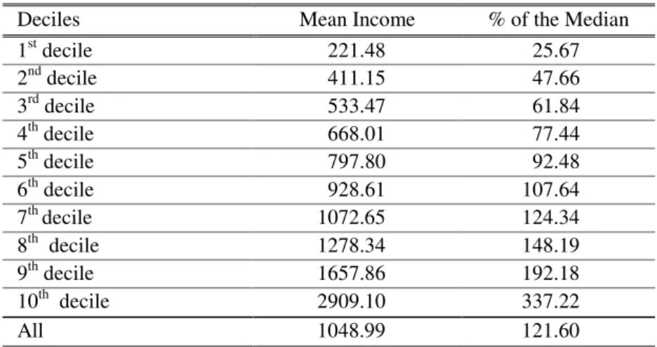
Table 7 represents the starting point for considering the distribution of individual incomes, based on the European Community Household Panel. It shows the equivalent income for the various deciles and for the distribution as a whole. It also shows the mean income of each decile as a percentage of the median.

Table 7 - Mean Income per Equivalent Adult by Deciles

Deciles Mean Income % of the Median

1st decile 221.48 25.67

2nd decile 411.15 47.66

3rd decile 533.47 61.84

4th decile 668.01 77.44

5th decile 797.80 92.48

6th decile 928.61 107.64

7th decile 1072.65 124.34

8th decile 1278.34 148.19

9th decile 1657.86 192.18

10th decile 2909.10 337.22

All 1048.99 121.60

(13)

Table 8 - Mean Income Shares per Equivalent Adult for each decile

Deciles Income Share Lorenz Curve

1st decile 0.02111 0.02111

2nd decile 0.03916 0.06027

3rd decile 0.05079 0.11106

4th decile 0.06381 0.17486

5th decile 0.07593 0.25079

6th decile 0.08865 0.33944

7th decile 0.10177 0.44121

8th decile 0.12174 0.56295

9th decile 0.15818 0.72113

10th decile 0.27887 1.00000

Tables 9 to 12 expand the analysis of the asymmetry in the income distribution to include the different social groupings under consideration.

If we look closely at Table 9, it can be seen that the households that consist of “one person aged 65 or more” and “single parent families with children aged less than 16” are those that have the lowest mean income per equivalent adult.

Table 9 - Mean Income per Equivalent Adult by Household Type

One person aged 65 or more 623.36

One person aged 30-64 1144.17

One person aged less than 30 1156.11

Single parent with 1 or more children (all children <16) 662.47 Single parent with 1 or more children (at least one >16) 1042.57 Couple without children (at least one aged 65 or more) 821.25 Couple without children (both aged less than 65) 1296.17 Couple with one child (child aged less than 16) 1280.87 Couple with two children (all children aged less than 16) 1141.25 Couple with >=3 children (all children aged less than 16) 855.68 Couple with >=1 children (at least one child >=16) 1059.35 Other type of household without family ties 996.35 Source:Own computation based on the ECHP-1995 micro-data; data are weighted.

(14)

Table 10 - Mean Income per Equivalent Adult by Region (NUT2)

Norte 975.33

Centro 861.06

Lisboa e Vale do Tejo 1328.83

Alentejo 852.38

Algarve 816.81

Açores 868.03

Madeira 753.24

Table 11 - Mean Income per Equivalent Adult by Rural/Urban Environment

Urban 1214.79

Semi-Urban 830.70

Rural 608.37

Finally, it can be seen from Table 12 that the households that have the lowest incomes are those where the main source of income is from social transfers.

Table 12 - Mean Income per Equivalent Adult by Main Source of Household Income

Wage and salary earnings 1166.09

Self-employment income 948.76

Pensions 796.93

Unemployment related benefits 687.40

Social benefits 517.95

Property, rental and capital income 1360.72

Other sources 1009.53

This great dispersion of incomes becomes more notable when the different inequality measures are considered.

Table 13 - Inequality Measures

Decile Ratio ( P90 / P10 ) 5.63921

Share Ratio ( S80 / S20) 7.25143

Gini Index 0.37064

Atkinson Index H=1.0 0.22139

Source: Own computation based on the ECHP-1995 and micro-data;data are weighted.

(15)

III.3. Characterisation of Households in a situation of Monetary Poverty

In order to identify exactly which households and individuals are in a situation of poverty, three poverty lines were constructed, corresponding to the income thresholds equivalent to 50%, 60% and 70% of the median income per equivalent adult. The following table shows the main results obtained:

Table 14 - Poverty Measures

Percentage of the Median

50% 60% 70%

Poverty Line 431.40 517.68 603.97

Head Count (D=0) 0.166651 0.238932 0.299759 Severity (D=1) 0.054960 0.079179 0.106871 Intensity (D=2) 0.029106 0.040734 0.054681 Source: Own computation based on the ECHP-1995 micro-data; data are weighted.

Taking the central figure of 60% as our reference, we can see that 24% of the population live in a situation of monetary poverty. This means that more than two million Portuguese, and roughly 875 thousand households, live in a situation of great precariousness, which makes it possible to classify them as poor12.

The following tables allow us to characterise the individuals that are in a situation of poverty in accordance with the socio-economic categories considered. Tables 15 to 18 show the percentage of poor people to be found in each of the groups (column A) and the distribution of the poor population throughout the various categories (column B).

Table 15 shows that the groups consisting of “one person aged 65 or more” and “single parents with children aged less than 16” are the ones with the highest shares of poor people. Couples with three or more children also show a high percentage of individuals in a situation of poverty.

Table 15 - Characterisation and Distribution of Poor People by Household Type

A B

One person aged 65 or more 57.3 6.4

One person aged 30-64 32.0 1.7

One person aged less than 30 13.9 0.1

Single parent with 1 or more children (all children <16) 49.9 2.1 Single parent with 1 or more children (at least one >16) 31.3 8.5 Couple without children (at least one aged 65 or more) 44.7 15.2 Couple without children (both aged less than 65) 25.1 6.0 Couple with one child (child aged less than 16) 10.1 3.8 Couple with two children (all children aged less than 16) 16.0 7.0 Couple with >=3 children (all children aged less than 16) 47.3 5.7 Couple with >=1 children (at least one child >=16) 19.5 28.4 Other type of household without family ties 20.5 15.1

All 23.9 100.0

12

(16)

The following table analyses the percentage of poor people in each of the seven regions of Portugal. Attention is drawn to the high proportion of individuals living in a situation of poverty in the Autonomous Regions of Açores and Madeira. In terms of spatial distribution, it is the northern region of the country which has the highest percentage of poor individuals (40.5% of the total population in a situation of poverty).

Table 16 - Characterisation and Distribution of Poor People by Region (NUT2)

A B

Norte 26.4 40.8

Centro 32.2 24.1

Lisboa e Vale do Tejo 11.9 16.0

Alentejo 31.9 7.8

Algarve 36.6 5.6

Açores 38.2 2.1

Madeira 37.4 3.6

All 23.9 100.0

Rural areas are the environments with a higher proportion of poor individuals. As we move from urban environments to rural environments, the poverty rate increases, reaching as high as 53.3% of the population living in rural areas.

Table 17 - Characterisation and Distribution of Poor People by Rural/Urban Environment

A B

Urban 14.8 39.8

Semi-Urban 33.0 32.4

Rural 53.3 27.8

All 23.9 100.0

Table 18 shows, once again, that it is those households whose main source of income consists of social transfers who live in the most fragile economic conditions, as well as having the highest poverty rates. 64.9% of poor individuals are to be found in those households where the main source of income is from social benefits. This percentage falls to 40.9% in those households where the main source of income is from pensions.

Table 18 - Characterisation and Distribution of Poor People by Main Source of Household Income

A B

Wage and salary earnings 15.1 40.5

Pensions 50.3 38.9

Unemployment related benefits 40.9 2.0

Social benefits 64.9 7.4

Property, rental and capital income 29.5 1.0

Other sources 43.2 0.7

All 23.9 100.0

(17)

IV Comparison between the European Community Household Panel and the Household Budget Survey

The aim of this section is to assess the consistency of results between the European Community Household Panel (1995) and the Household Budget Survey (94/95) 13 in analysing income distribution, inequality and poverty.

In making this comparison between these two sources of information, it should be borne in mind that there are important differences resulting not only from the quite distinct (and differently-sized14) samples, but also from the different concepts and methodologies used. Consequently, this comparison does not necessarily give rise to one of them being chosen as a preferred tool for studying the living conditions of households. The identification and perception of the differences existing between the two surveys may, however, represent an important step towards the future improvement and perfection of them both.

Two aspects will be analysed in detail here: the population structure and the income structure represented in each of the surveys.

IV.1 Population Structure

As far as the population structure is concerned, Tables 19 to 22 allow us to compare the results of the surveys.

Table 19 shows the distribution of households and individuals by household type. The divergences between the two surveys seem to us to be perfectly acceptable, given the different samples.

Table 19 - Comparison between the ECHP (1995) and the HBS (94/95) - Household Type (%)

Households Individuals

ECHP HBS ECHP HBS

One person aged 65 or more 8.1 10.0 2.7 3.3

One person aged 30-64 4.2 3.8 1.4 1.3

One person aged less than 30 0.4 0.2 0.1 0.1

Single parent with 1 or more children (all children <16) 1.1 1.3 1.0 1.1 Single parent with 1 or more children (at least one >16) 7.7 5.3 6.5 4.8 Couple without children (at least one aged 65 or more) 12.2 14.6 8.1 9.7 Couple without children (both aged less than 65) 8.9 7.6 5.9 5.1 Couple with one child (child aged less than 16) 9.0 8.1 9.0 8.1 Couple with two children (all children aged less than 16) 7.8 6.6 10.3 8.7 Couple with >=3 children (all children aged less than 16) 1.6 1.8 2.9 3.2 Couple with >=1 children (at least one child >=16) 26.9 29.1 34.7 39.1 Other type of household with family ties 12.0 10.6 17.6 14.4 Other type of household without family ties 0.0 0.9 0.0 1.3

All 100.0 100.0 100.0 100.0

Source: Own computation based on the ECHP-1995 and HBS 1994-95 micro-data; data are weighted.

13

For a description of the Household Budget Survey 1994/95 see INE (1997).

14

(18)

The following two tables compare population structure on the basis of regional distribution and rural/urban environments.

Table 20 - Comparison between the ECHP (1995) and the HBS (94/95) – Region (%)

ECHP HBS ECHP HBS

Norte 34.6 32.4 37.0 35.5

Centro 18.5 18.1 17.9 17.3

Lisboa e Vale do Tejo 33.0 35.4 32.0 33.4

Alentejo 6.3 5.9 5.8 5.3

Algarve 4.3 3.9 3.8 3.5

Açores 1.1 2.1 1.3 2.4

Madeira 2.2 2.2 2.3 2.6

All 100.0 100.0 100.0 100.0

Table 21 - Comparison between the ECHP (1995) and the HBS (94/95) - Rural/Urban Environment (%)

ECHP HBS ECHP HBS

Urban 63.2 55.8 63.9 55.8

Semi-Urban 22.2 26.0 23.5 27.5

Rural 14.7 18.2 12.6 16.8

All 100.0 100.0 100.0 100.0

Although the structure by regions is very similar in the two cases, the two surveys do, however, reveal sharp differences in the relative importance that each of them gives to the individuals and households living in rural and urban environments. The HBS unequivocally gives a higher share to rural populations than does the ECHP. As we shall see, this divergence in population structure is inevitably reflected in income structure.

(19)

Table 22 - Comparison between the ECHP (1995) and the HBS (94/95) Main Source of Household Income (%)

ECHP HBS-MI HBS-TI ECHP HBS-MI HBS-TI

Wage and salary earnings 55.2 48.9 46.7 64.1 58.3 55.8

Self-employment income 10.6 13.5 11.7 12.3 15.9 13.9

Pensions 28.0 31.9 28.9 18.4 20.7 18.9

Unemployment related benefits 1.2 1.1 1.0 1.2 1.1 1.0

Social benefits 3.3 0.3 0.3 2.7 0.4 0.3

Property, rental and capital income 1.2 1.8 1.4 0.8 1.4 1.1

Other sources 0.5 2.4 10.1 0.4 2.2 9.1

All 100.0 100.0 100.0 100.0 100.0 100.0

As can be seen from the above table, the ECHP shows a larger percentage of the population living in households whose main source of income is from wage and salary earnings, which may well be linked to the greater share of urban families in the Panel. When the population structure of the Panel is compared to the equivalent structure of the HBS (HBS - Monetary Income), it should be noted that a greater percentage of the population of the ECHP is also to be found in households where the main source of income is from Social Benefits. The Panel gives greater attention to surveying the different types of social transfers and this may be a plausible explanation for the differences to be found under this heading in the two surveys.

If we take into account all the items of income that are surveyed under the HBS (HBS - Total Income), then the number of households and individuals whose main source of income appears in the “Other Sources” category rises to 9-10% and makes it possible to anticipate the importance that non-monetary incomes have in household income.

IV.2. Income Structure

In comparing income structure between the ECHP and the HBS, we must take into account the different concept of household income underlying each of the surveys. As we have seen, the basic concept used by the Panel is that of Net Monetary Household Income, whilst the basic concept in the Household Budget Survey is that of Total Net Income, which includes both monetary and non-monetary income. In order to ensure the comparability of the analysis, Table 23 shows three household income structures:

i) the Panel’s monetary income structure;

ii) the HBS monetary income structure (HBS - Monetary Income), which is compatible with that of the ECHP;

iii) the HBS total income structure (HBS - Total Income).

(20)

A second aspect that emerges from a study of Table 23 is the greater relative importance of wage and salary earnings in the Panel’s monetary income structure. This fact is consistent with the earlier analysis of population distribution according to the main source of household income and justifies more detailed future research into the causes for this situation, namely with regard to how the samples are constructed for the two surveys.

Table 23 - Comparison between the ECHP (1995) and the HBS (94/95) Household Income Structure

Income Source ECHP (%) HBS-MI (%) HBS-TI (%)

Wage and salary earnings 1284.3 63.5 1123.2 55.9 1123.2 45.8 Self-employment income 222.2 11.0 302.7 15.1 302.7 12.3 Total net income from work 1506.5 74.4 1425.8 70.9 1425.8 58.1

Capital income 36.4 1.8 24.6 1.2 24.6 1.0

Property and rental income 15.9 0.8 33.9 1.7 33.9 1.4

Private transfers received 9.5 0.5 68.0 3.4 68.0 2.8

Non-work private income 61.8 3.1 126.5 6.3 126.5 5.2

Unemployment related benefits 30.1 1.5 33.6 1.7 33.6 1.4 Old-age and survivors benefits 351.9 17.4 391.6 19.5 391.6 16.0

Family-related allowances 30.7 1.5 19.1 1.0 19.1 0.8

Sickness and invalidity benefits 37.5 1.9 7.1 0.4 7.1 0.3

Education-related benefits 2.1 0.1 2.4 0.1 2.4 0.1

Any other (personal) benefits 2.9 0.1 4.5 0.2 4.5 0.2

Social assistance 0.2 0.0 0.0 0.0 0.0 0.0

Housing allowance 0.2 0.0 0.0 0.0 0.0 0.0

Social Transfers 455.4 22.5 458.3 22.8 458.3 18.7

Monetary income 2023.7 100.0 2010.6 100.0 2010.6 82.0

Wages in kind (-) (-) 20.2 0.8

Autoconsumption (-) (-) 67.7 2.8

Imputed rents (-) (-) 263.1 10.7

Other nom monetary income (-) (-) 90.4 3.7

Non-Monetary Income (-) (-) 441.4 18.0

Total Income (-) (-) 2452.0 100.0

One final aspect that should also be stressed is the importance of non-monetary income in the Total Net Household Income. According to the HBS, in 1994, such income represented 18% of total income, so that the fact that it is not considered by the Panel implies a clear underestimation of the resources enjoyed by the population, with the obvious consequences that this has on their level of welfare.

IV.3. Inequality and Poverty Levels

(21)

Returning once more to the question of individual income distribution per equivalent adult, Tables 24 to 26 show the different indicators for income distribution, inequality and poverty.

Table 24 - Comparison between the ECHP (1995) and the HBS (94/95) Shares of Total Income for each Decile

ECHP HBS-MI HBS-TI

1st decile 0.02111 0.02766 0.02973

2nd decile 0.03916 0.04230 0.04415

3rd decile 0.05079 0.05302 0.05512

4th decile 0.06381 0.06422 0.06468

5th decile 0.07593 0.07472 0.07446

6th decile 0.08865 0.08618 0.08624

7th decile 0.10177 0.10050 0.09972

8th decile 0.12174 0.11876 0.11915

9th decile 0.15818 0.15229 0.15310

10th decile 0.27887 0.28036 0.27364 Source: Own computation based on the ECHP-1995 and HBS 1994-95 data; data are weighted.

Table 25 - Comparison between the ECHP (1995) and the HBS (94/95) Inequality Measures

ECHP HBS-MI HBS-TI

Decile Ratio ( P90 / P10 ) 5.63921 4.93145 4.69922 Share Ratio ( S80 / S20) 7.25143 6.18499 5.77587

Gini Index 0.37064 0.35749 0.34713

Atkinson Index H=1.0 0.22139 0.19429 0.18150 Atkinson Index H=1.5 0.32938 0.27443 0.25452 Atkinson Index H=2.0 0.44404 0.35185 0.32032 Source: Own computation based on the ECHP-1995 and HBS 1994-95 data; data are weighted.

Table 26 - Comparison between the ECHP (1995) and the HBS (94/95) Poverty Measures (60% of Median)

ECHP HBS-MI HBS-TI

Poverty Line 517.68 499.10 608.52

Head Count (D=0) 0.238932 0.203907 0.180466 Severity (D=1) 0.079179 0.053664 0.046198 Intensity (D=2) 0.040734 0.021675 0.017508 Source: Own computation based on the ECHP-1995 and HBS 1994-95 data; data are weighted.

(22)

In comparing the monetary income distribution between the two surveys, it can be seen that the Panel shows a level of inequality, measured by the Gini Index, that is roughly one and a half percentage points higher than that recorded in the HBS. The different values of the Atkinson Index confirm this deviation, also showing that this gap is even larger for higher values of ε. The behaviour suggested by the Atkinson Index is that the increasing inequality shown by the Panel may be partly explained by a lower level of relative income in the first deciles of the distribution of the ECHP in comparison with those of the HBS. An observation of the share of total income for each decile (Table 24) helps to confirm this explanation.

As far as the poverty rate is concerned, and taking into account the reference value of 60% of the median income as the poverty threshold, the Panel also shows a greater share of poor individuals: 23.9% of the population in comparison with the 20.4% estimated by the HBS.

A possible explanation for the greater inequality and higher levels of poverty in the individual distribution of per equivalent monetary income shown by the Panel may be found in the income structure of the two surveys. In an earlier study15, we showed that the pay inequalities in Portugal had an impact on total inequality that was more than proportional to their share of the income structure. Given the greater share of wage and salary earnings in the Panel’s income structure, it does not seem strange to us that this greater share should result in a higher level of inequality.

The comparison between the distribution of monetary income and total income shows that, in the Portuguese case, the group of different non-monetary incomes has an equalising effect on income distribution and the level of inequality, and that this is particularly significant in the first deciles of income distribution, as can be seen in the last two columns of Table 24.

Consideration of non-monetary income has equally important repercussions on the determination of the poverty rate. If we consider all household incomes together, the poverty rate recorded by the HBS is 18%, roughly 6 percentage points lower than the figure arrived at using the Panel’s monetary income distribution. This once again highlights the importance in Portugal of non-monetary incomes in relation to the total income and living conditions of families, particularly amongst low-income families.

V - Main Results and Guidelines for Future Research

Firstly, this study has highlighted the fact that there was a high level of asymmetry in income distribution in Portugal in 1994, characterised by high levels of inequality and linked to very significant situations of precariousness and monetary poverty. These results have proved to be sufficiently robust and are not dependent on the source of statistical information used. Both the European Community Household Panel and the Household Budget Survey show levels of inequality and poverty that are far higher than those recorded in most EU countries.

15

(23)

A second aspect that should be borne in mind has to do with the use of the European Community Household Panel in the analysis of household income distribution and living conditions. As the Panel is the most important repository of information on households and individuals in Portugal, this study embodies a first attempt to model its micro-economic data in the analysis of income distribution and in the identification of families in situations of poverty. The consistency test conducted on the results obtained, by comparing these with the ones provided by the HBS, not only confirms the potentialities of using the Panel as a special tool for the study of family living conditions, but also shows that the Panel may provide a frame of reference for the harmonisation and improvement of the system of statistics on families and households.

(24)

References

Atkinson, A. B. (1970) "On the Measurement of Inequality," Journal of Economic Theory, 244-63.

Atkinson, A. B. (1983), The Economics of Inequality (2nd Ed).

Atkinson, A. B. (1990) "On the Measurement of Poverty," Econometrica, 749-764.

Costa, A. Bruto da (1994), "The Measurement of Poverty in Portugal", Journal of European Social Policy, 4, 2, 95- 115.

Cowell, F. (1994), Measuring Inequality, LSE Handbooks in Economics, London, 2nd Ed.

Eurostat (1996), The European Community Household Panel (ECHP): Vol.1 – Survey methodology and Implementation, Theme 3, Series E, Eurostat, OPOCE, Luxemburgo .

Eurostat (1998a), “ECHP Data Quality”, mimeo.

Eurostat (1998b), “Analysis of Income Distribution in 13 EU Member States”, Statistics in Focus – Population and Social Conditions, 1998-11.

Ferreira, L. (1992), “Pobreza em Portugal - Variação e Decomposição de Medidas de Pobreza a partir dos Orçamentos familiares de 1980-1981 e 1989-1990”, Estudos de Economia, 12, 4, 377-393.

Foster, J., Greer,J. and Thorbecke,E. (1984), “A Class of Decomposable Poverty Measures”, Econometrica; 52(3), 761-66.

Gouveia, M. and J. Tavares (1995), "The Distribution of Household Income and Expenditure in Portugal: 1980 and 1990", Review of Income and Wealth, 41 (1), 1-19, 1995.

INE (1997), Metodologia do Inquérito aos Orçamentos Familiares 1994-1995, Lisboa, 1997

Rodrigues, C.F. (1993), The Measurement and Decomposition of Inequality in Portugal [1980/81 - 1989/90]“, Microsimulation Unit Discussion Paper MU9302, Cambridge, Department of Applied Economics.

Rodrigues, C. F. (1994), “Repartição do Rendimento e Desigualdade: Portugal nos anos 80”, Estudos de Economia, 14, 4, 399-427.