Received: 14 September 2012 / Accepted: 02 April 2013 / Available (online): 13 June 2013 / Published: 01 December 2013
Longitudinal Study in Male Swimmers: A Hierachical Modeling of Energetics
and Biomechanical Contributions for Performance
Mário J. Costa 1,6 , José A. Bragada 2,6, Daniel A. Marinho 3,6, Vitor P. Lopes 2,6, António J. Silva 4,6
and Tiago M. Barbosa 5,6
1 Polytechnic Institute of Setúbal, Setúbal, Portugal; 2 Polytechnic Institute of Bragança, Bragança, Portugal; 3 University of Beira Interior, Covilhã, Portugal; 4 University of Trás-os-Montes and Alto Douro, Vila Real, Portugal; 5 National Institute of Education, Nanyang Technological University, Singapore; 6 Research Centre in Sports Science,
Health and Human Development, Vila Real, Portugal Abstract
The aim of this study was to assess the pooled and individual response of male swimmers over two consecutive years of training and identify the energetic and biomechanical factors that most contributed for the final performance. Nine competitive swimmers (20.0 ± 3.54 years old; 10.1 ± 3.41 years of training experience; 1.79 ± 0.07 m of height; 71.34 ± 8.78 kg of body mass; 22.35 ± 2.02 kg·m-2 of body mass index; 1.86 ± 0.07 m of arm span; 116.22 ± 4.99 s of personal record in the 200 m long course freestyle event) performed an incremental test in six occasions to obtain the velocity at 4 mmol of blood lactate (V4) and the peak blood lactate concentrations (Lapeak) as energetics, and the stroke frequency (SF), stroke length (SL), stroke index and swim efficiency as biomechanical variables. Performance was determined based on official time’s lists of 200 m freestyle event. Slight non-significant improvements in performance were determined throughout the two season period. All energetic and biomechanical factors also presented slight non-significant variations with training. Swimmers demonstrat-ed high inter-individual differences in the annual adaptations. The best performance predictors were the V4, SF and SL. Each unit of change V4, SF and SL represented an enhancement of 0.11 s, 1.21 s and 0.36 s in performance, respectively. The results show that: (i) competitive male swimmers need at least two consecutive seasons to have slight improvements in performance, energetics and biomechanical profiles; (ii) major improvements in competition performance can be accomplished by improving the V4, SF and SL based on the individual background.
Key words: Male swimmers, tracking, training, testing, annual changes.
Introduction
The ability to monitor changes within and between seasons provides fundamental information for coaches about the status of their swimmers. Energetics and biomechanical data are crucial to determine the effectiveness of their training periodization and therefore adjust training methods in order to enhance performance (Costa et al., 2012a). Among the energetics data assessed on a regular basis are the velocity at 4 mmol of blood lactate concentrations (V4) and the maximal blood lactate concentrations after exercise (Lapeak). The assessment of V4 and Lapeak status throughout the season is determinant while monitoring the aerobic and anaerobic fitness of the
swimmers, respectively. It was demonstrated that the aerobic fitness in high level swimmers can be improved with training. Adult male swimmers are able to display a small but meaningful increase in V4 of ~1.5% within the season (Pyne et al., 2001; Anderson et al., 2006; Costa et al., 2012b). Most of those gains in aerobic fitness occur in the early months, due to an increase in training volume (Sharp et al., 1984). Adaptations in anaerobic fitness are also evident throughout a training season. Increases in Lapeak (from ~12% to ~27%) have been reported in competitive male swimmers (Anderson et al., 2006; Faude et al., 2008; Termin and Pendergast, 2000). Conversely, those changes seem only to occur from mid phases until the season’s end (Faude et al., 2008).
Most of the longitudinal evidences regarding biomechanical factors were based in the stroke frequency (SF) and stroke length (SL) adaptations. However, some inconsistent findings between studies were presented. Anderson et al. (2006) reported that male swimmers tend to increase SF and decrease SL in 1% to 2% each year. The authors also reported a large gender and competitive level in response to training. On the other hand, Costa et al. (2012b) determined within season increases (~2%) in SL and decreases (~1.3%) in SF for international and national level swimmers. Researchers have also focused their attention on other biomechanical measures, such as the stroke index (SI) and the swim efficiency (ηp). Both variables showed to increase with training, namely in the last stage of the season in such athletes (Costa et al., 2012b).
Nevertheless, most of the studies above mentioned only tracked performance, energetics and biomechanical profiles during one single season or a shorter time period. Considering the state of the art in training-intervention studies, the scientific literature suggests that changes in competitive athletes occur very smoothly. It is quite difficult to observe in this population meaningful increases in performance, energetic or biomechanical profiles in just one single season. Therefore, it is important to determine the swimmers adaptations to training throughout longer field interventions. Added to that, the assessment of individual trends is another important topic of training diagnosis and should also be for sport performance researchers. With the identification of the energetic and biomechanical factors that most contribute for the final performance, and the swimmer’s
adequate prescription for further improvements.
In this sense, the aim of this study was to: (i) assess the pooled and individual response of male swimmers over two consecutive years of training; (ii) identify the energetic and biomechanical factors that most contributed for the final performance.
Methods
Participants
Twelve competitive male simmers were recruited to participate in the present study. Three swimmers were excluded because of an acute muscle-skeletal injury (n = 1), changed to another swimming team (n = 1) and withdrawal from swimming career (n = 1). A total of nine swimmers (20.0 ± 3.54 years old; 10.1 ± 3.41 years of training experience; 1.79 ± 0.07 m of height; 71.34 ± 8.78 kg of body mass; 22.35 ± 2.02 kg m-2 of body mass index; 1.86 ± 0.07 m of arm span; 116.22 ± 4.99 s of personal record in the 200 m long course freestyle event) were considered for further analysis. The elite nature of the participants is indicated by the presence in Athens 2004 Olympic Games and Melbourne 2007 World Swimming Championships (n = 1), Rome 2009 World Swimming Championships (n = 2) and 2010 LEN Multinations Junior Meet (n = 1) representing their National Swimming Team. Collectively, the other half of the group (n = 5) were top 20 nationally-ranked in the 200 m freestyle event. All swimmers gave their written informed consent before participation, and procedures had the approval from the scientific board of the Polytechnic Institute of Bragança for human studies.
Study design
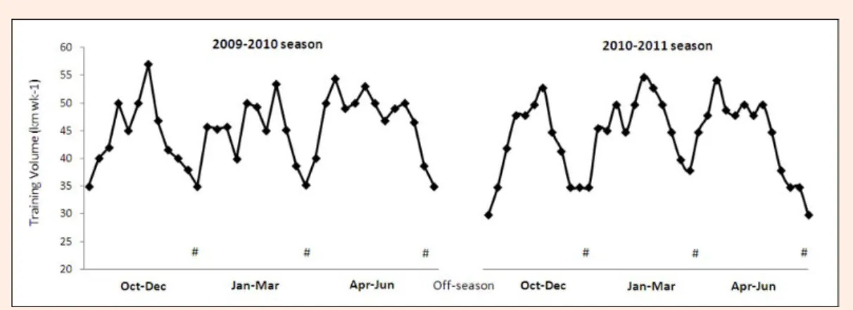
The nine swimmers were studied in six occasions (n = 54 tests, six tests per swimmer, spaced three months each) over two consecutive years of training (2009-2010 and 2010-2011 seasons). The six tests were conducted at the end of the following time periods: (i) October-December 2009 (TP1); (ii) January-March 2010 (TP2); (iii) April-June 2010 (TP3); (iv) October-December 2010 (TP4); (v) January-March 2011(TP5) and; (vi) April-June 2011 (TP6). Weekly training volume (Figure 1) averaged 44 ± 7 km·wk-1 and 45 ± 6 km·wk-1 for the first and second
consisted in nine sessions per week involving low, medium and high aerobic tasks, intense sprint work and technical drills. There was an increase in training intensity from the first to the second season namely in: (i) intensity corresponding to their aerobic capacity (2009-2010: 2.02 ± 0.42 km·wk-1; 2010-2011:2.73 ± 0.74 km·wk-1); (ii) intensity corresponding to their aerobic power (2009-2010: 1.22 ± 0.21 km·wk-1; 2010-2011: 1.65 ± 0.14 km·wk-1) and; (iii) anaerobic capacity training (2009-2010: 0.94 ± 0.54 km·wk-1; 2010-2011: 1.04 ± 0.26 km·wk-1). In the day prior to data collection, the swimmers completed a low intensity training session in order to avoid data bias due to fatigue.
Energetic and biomechanical data collection
An incremental n x 200 m step test (n<8) until exhaustion (Fernandes et al., 2003) on a long course pool was used to evaluate the swimmer’s energetic and biomechanical adaptations. Warm up procedures were standardized before each test. The starting velocity was set at a speed, which represented a low training pace, approximately 0.3 m s-1 less than the swimmer’s best performance. The increments in velocity were chosen, so that swimmers would attain their best performance on the last trial. Underwater pacemaker lights (GBK-Pacer, GBK Electronics, Aveiro, Portugal) on the bottom of the pool were used to control the swimming velocity and to help the swimmers keep an even pace along each lap and step. In addition, elapsed time for each trial was measured with a chronometer to control the swimmer’s velocity.
Capillary blood samples were taken from the ear lobe during the 30 s resting period between trials, immediately following and in the 3rd, 5th, and 7th min after of the intermittent protocol. Samples were then analyzed for lactate concentrations (YSI 1500 L, Yellow Springs, Ohio, USA).
The energetical profile was analyzed in terms of aerobic and anaerobic fitness and quantified based on the V4 (in m s-1) and the Lapeak (in mmol L-1) assessments. The individual V4 was obtained by interpolation of the average lactate value (4 mmol l-1) on the exponential curve of lactate/speed relationship. The Lapeak was consi-dered to be the highest blood lactate concentration in post exercise condition (Termin and Pendergast, 2000).
The biomechanical profile was determined based on the measurement of the SF (in Hz), SL (in m), SI (in m2.c-1.s-1) and η
p (in %). The SF was recorded manually from three consecutive stroke cycles in the middle of each lap during each trial, using a crono-frequency meter (Golfinho Sports MC 815, Aveiro, Portugal). Since most of the SF values recorded by researchers were practically equal, the degree of agreement was not examined. Then, SF values were converted to International System Units (i.e. Hz). The SL was estimated as (Craig et al., 1985):
SF
v
SL = (1)
where SL is the stroke length (in m), v is the swimming velocity (in m.s-1), and the SF is the stroke frequency (in Hz).
The SI is considered as one of the swimming stroke efficiency indexes and was computed as (Costill et al., 1985):
SL v
SI= ⋅ (2)
where SI is the stroke index (in m2·c-1·s-1), v is the swimming
velocity (in m·s-1) and the SL is the stroke length (in m).
The ηp was also estimated based on (Zamparo et al., 2005): π . l π . 2 SF 2 9 0 v ηp ⋅ ⋅ ⋅ = (3)
where v is the swimming velocity (in m·s-1), the SF is the stroke
frequency (in Hz) and l is the arm’s length (in m). The l is computed trigonometrically measuring the arm’s length and considering the average elbow angles during the insweep of the arm pull as reported by Zamparo (2006). This is considered an approximation of the Froude efficiency.
All the energetic and biomechanical data were then corrected by interpolation to the mean swimming velocity reached in competition conditions.
Performance data collection
Whenever possible, swimming performance was assessed based on times lists of the 200 m freestyle event during official long course competitions from local, regional, national and/or international level. However, in earlier months of the season most of the competitions take place on short course swimming pools. The most easy and operational way to convert the short course race times in long course race times was to use specific software tool (FINA converter). This is a common approach used by most of the Swimming National Federations to convert race times for national and international meetings. The time between the official competition performances and the testing day never exceeded two weeks.
Statistical analysis
Data was expressed as mean and standard deviation and quartiles for each time period. Within and between season changes in performance, energetic and biomechanical variables were analyzed with Friedman Test, as well as the Wilcoxon Signed-Rank Test. The relative frequency
of change (%) for each season was also reported. Ranking Spearman Correlation Coefficients (rs) were used to assess the stability between seasons. Cohen’s Kappa tracking index (K) was obtained in the Longitudinal Data Analysis software (v. 3.2, Dallas, USA) and used to detect inter-individual differences over the season. The K was computed based on three growth curves (“tracks”) delimited by the percentiles 33, 66 and 100. The number of times that each swimmer goes out of a specific track reflects the inter-individual stability in a certain characteristic. The qualitative interpretation of K values was made according to Landis and Koch suggestion (1977), where the stability is: (i) excellent if K ≥ 0.75; (ii) moderate if 0.40 ≤ K < 0.75 and; (iii) low if K < 0.40. Since repeated measures were nested within subjects, the longitudinal data set was treated as hierarchical. A two-level HLM was used to model the performance changes along the two consecutive seasons. The HLM creates a hierarchical structure like a “tree”, being able to identify the energetics and biomechanical variables as performance changing predictors. This approach has been already used in other competitive sports (Bragada et al., 2010) and other scientific disciplines (Lopes et al., 2011) for such purpose. Nevertheless, it was never attempted in competitive swimming. The first step to model performance in the HLM framework consisted in modeling the changes in performance over the two seasons. In this step only time was include as predictor. The second step consisted in testing the energetics and biomechanical variables as swimming performance changing predictors. Maximum likelihood estimation was used with the HLM5 statistical software (Raudenbush and Bryk, 2002) which computes robust standard errors, a convenient option in this study due to small sample size. Also due to small sample size only the fixed effects were considered (Mass and Hox, 2004). Effect size was computed based on Eta-squared (η2) procedure, and values interpreted according to Ferguson (2009) being: without effect if 0 < η2 < 0.04; minimum if 0.04 < η2 < 0.25; moderate if 0.25 < η2 < 0.64 and; strong if η2 > 0.64. The level of statistical significance was set at P ≤ 0.05. Whenever data was (Winter, 2008): (i) significant (P ≤ 0.05) with at least with a minimum effect size (η2 > 0.4) it was reported as being a “meaningful variation”; (ii) non significant (P > 0.05) with a minimum or without effect size (η2 ≤ 0.25) it was reported as being a “slight variation”.
Results
Changes within and between seasons
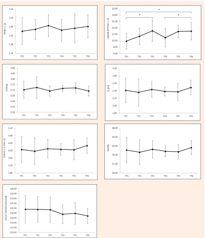
Figure 2 presents the changes in energetics, biomechanics and performance. All energetics and biomechanical variables presented slight non-significant variations within and between seasons (V4, p = 0.44, η2 = 0.03; Lapeak, p = 0.05, η2 = 0.19; SF, p = 0.52, η2 = 0.05; SL, p = 0.32, η2 = 0.03; SI, p = 0.15, η2 = 0.03; η
p, p = 0.34, η2 = 0.03). The performance also presented a slight non-significant improvement during such time period (200m, p = 0.14; η2 = 0.06).
Figure 2. Variations on energetics, biomechanics and performance throughout the two years of training. * indicates significant
different from TP1 to TP3 (p = 0.02), from TP4 to TP6 (p = 0.05) and from TP1 to TP6 (p = 0.02).
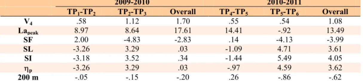
Table 1 presents the relative changes (%) on energetics, biomechanics and performance throughout the two consecutive seasons. The energetic and biomechanical variables with higher change were the Lapeak (1st season = 17.61%; 2nd season = 13.49%) and the SI (1st season = 0.34%; 2nd season = 4.05%), respectively. While for the energetic profile most of the gains were obtained in the first season, in the biomechanical profile the higher range of variation was most notorious in the
second one.
Inter-individual variations within and between seasons
Table 2 presents the auto-correlation Spearman Correlation Coefficients for energetics and biomechanic selected variables. Most of the variables presented high stability (rs > 0.60) throughout the two consecutive seasons. High associations were found in adjacent time periods (e.g. TP1 vs TP2) or in similar time periods but
Table 1. Relative change (%) on energetics, biomechanics and performance within each year of training. 2009-2010 2010-2011 TP1-TP2 TP2-TP3 Overall TP4-TP5 TP5-TP6 Overall V4 .58 1.12 1.70 .55 .54 1.08 Lapeak 8.97 8.64 17.61 14.41 -.92 13.49 SF 2.00 -4.83 -2.83 .14 -4.13 -3.99 SL -3.26 3.29 .03 -1.09 4.71 3.61 SI -3.18 3.52 .34 -1.44 5.49 4.05 ηp -3.26 3.29 .03 -.97 4.59 3.62 200 m -.05 -.15 -.20 .26 -.86 -.62
V4, velocity at 4 mmol of lactate levels; Lapeak, maximal blood lactate concentration; SF, stroke frequency; SL, stroke
length; SI, stroke index; ηp, propelling efficiency; 200 m, freestyle performance time in competition.
from separate seasons (e.g. TP3 vs TP6).
The inter-individual assessment based on K values showed low stability for the Lapeak (K = 0.24 ± 0.12), SF (K = 0.17 ± 0.12), SL (K = 0.30 ± 0.12) and ηp (K = 0.26 ± 0.12). Moderate values were verified for the V4 (K = 0.42 ± 0.12), SI (K = 0.49 ± 0.12) and 200 m performance (K = 0.60 ± 0.12).
Hierarchic linear modeling
In the HLM the linear, quadratic and cubic changes were tested. However, only linear change was significant (Table 3). The retained performance predictors from biomechanical domain were the SL and SF, while from the energetic was the V4. The model shows that the mean of initial swimming performance was 119.28 s and improved linearly 0.35 s between each evaluation. The V4 had a positive impact in performance, suggesting that for each unity change (in cm.s-1) the swimming performance improved 0.11 s. The SL and SF had also a positive impact in performance. For each unity of change in SL (in cm) swimming performance improved 0.36 s, and for each unity of change in SF (in Hz), swimming performance improved 1.21 s.
Discussion
The purpose of this study was to assess the pooled and individual response of male swimmers over two consecutive years of training and identify the energetics and biomechanical factors that most contributed for the final performance during such time frame. The main result was that only slight variations were observed in the swimmers’ performance, energetics and biomechanical profiles within and between seasons. Each swimmer responded differently to training. The best longitudinal performance predictors were the V4, SL and SF.
Changes within and between seasons
Within and between seasons non-significant adaptations were determined for the energetic variables. There was a slight increase in V4 of ~1.7% and ~1.1% in the first and second seasons, respectively. Earlier observations have already reported small increases in high-level male and female swimmer’s V4 of ~1.5% after several months of training (Anderson et al., 2006; Costa et al., 2012b; Pyne et al., 2001). The training induces muscle adaptations and improves the muscle’s ability to produce energy aerobically (Madsen, 1983). However, due to several years/decade of systematic and hard training the margin for further aerobic improvement in high-level athletes is quite small (Houston et al., 1981).
Table 2. Interperiod Spearman Correlation Coefficients of energetic and biomechanical variables over the two years of training. V4 TP1 TP2 TP3 TP4 TP5 TP6 Lapeak TP1 TP2 TP3 TP4 TP5 TP6 TP1 1 TP1 1 TP2 .77* 1 TP2 .17 1 TP3 .42 .33 1 TP3 .27 .45 1 TP4 .95** .70* .46 1 TP4 .37 .30 .32 1 TP5 .73 .63 .64 .82** 1 TP5 .30 .43 .92** .37 1 TP6 .64 .73* .59 .60 .84** 1 TP6 .23 .38 .47 .70* .48 1 SF TP1 TP2 TP3 TP4 TP5 TP6 SL TP1 TP2 TP3 TP4 TP5 TP6 TP1 1 TP1 1 TP2 .58 1 TP2 .64 1 TP3 .75* .32 1 TP3 .77* .58 1 TP4 .20 -.02 .44 1 TP4 .51 .58 .84** 1 TP5 .66 .74* .60 .25 1 TP5 .63 .83** .67* .53 1 TP6 .49 .08 .61 .09 .59 1 TP6 .58 .35 .80** .57 .67* 1 SI TP1 TP2 TP3 TP4 TP5 TP6 ηp TP1 TP2 TP3 TP4 TP5 TP6 TP1 1 TP1 1 TP2 .60 1 TP2 .60 1 TP3 .73* .70* 1 TP3 .87** .42 1 TP4 .60 .70* .92** 1 TP4 .57 .12 .80** 1 TP5 .72* .87** .60 .58 1 TP5 .82** .73* .65 .25 1 TP6 .78* .60 .63 .58 .87** 1 TP6 .77* .27 .78* .45 .72* 1 * p < 0.05; ** p < 0.01
standard errors (SE) and confidence intervals.
Parameter Estimate(SE) 95% Confidence Interval
First model Intercept 119.88 (1.42) 116.74 — 120.01 Time -.59 (.16) -.90 — -.27 Last model Intercept 119.27 (.37) 118.49 — 120.06 Time -.35 (.09) -.53 — -.16 V4 -.10 (.04) -.20 — -.55 SL -.36 (.02) -.41 — -.31 SF -1.21 (.08) -1.38 — -1.04
V4, velocity at 4 mmol of lactate levels; SL, stroke length; SF, stroke frequency
The Lapeak also presented a slight improvement. Training induces muscle anaerobic adaptations allowing higher velocities at an increased oxygen debt and muscle reduced fatigue (Termin and Pendergast, 2000). The mean percentage of variation was ~18% and ~14% in the first and second years, respectively. Those values are in accordance with previous observations (from ~12% to ~27%) from male swimmers with similar competitive level (Anderson et al., 2006; Faude et al., 2008; Termin and Pendergast, 2000). The Lapeak can also be dependent on the motivational commitment with the exercise. It can be speculated, at least is a current topic of discussion among practioners that the marginally higher Lapeak can be due to a higher motivation resulting in a higher effort. So, this energetic measure is extremely sensitive and should be interpreted with caution.
For the biomechanical variables, slight non-significant variations were observed over the two consecutive years. The SF decreased ~3% and ~4% within the first and second seasons, respectively. Conversely, the SL increased ~0.1% and ~4% throughout those time periods. A small magnitude of change has already been determined for international and national male swimmers within one single season (Costa et al., 2012b). This SF and SL relationship throughout several months seems to depend on the training characteristics. The high volume programs have been found to increase SL but not the SF of well trained male swimmers (Costa et al., 2012b; Costill et al., 1991; Wakayoshi et al., 1993). While swimming at lower speeds, subjects can focus on stroke phase aspects, and therefore increase the distance swum per stroke. However, such programs do not seem to develop so easily the muscular power and strength (Dudley and Fleck, 1987). An increase in training intensity in the second season was determinant to change SF and SL in a higher range than in the first one. In overall perspective, the kinematical combination demonstrated by the present athletes is in accordance with the strategy adopted by elite swimmers that made them more efficient than lower level ones (Costa et al., 2012b). An increase in swimming stroke efficiency throughout the study was demonstrated by both indexes. The SI and ηp increased ~4% and 3% during the two years of training, respectively. The SI depends on the velocity and SL adaptations (Costill et al., 1985). A higher SI over the season represented an improved ability to swim at similar velocities traveling higher distances within a stroke cycle. On the other hand, the ηp is determined by the
relationship between velocity and SF (Zamparo et al., 2005). Seasonal adaptations allowed the swimmers to reach similar velocities with fewer strokes. Previous studies have also reported efficiency increases in international and national level male swimmers during one single season (Costa et al., 2012b). However, the variation in both indexes (2 to 3%) was lower than in the present study. It seems that the duration of the intervention is a major factor influencing the magnitude of change.
The swimmers became slightly faster within and between seasons. Their race times slightly improved 0.20% and 0.60% on average in the first and second seasons, respectively. A lack of improvement, or a small magnitude in the performance of high-level male swimmers, has been published in a couple of other papers as well (Costil et al., 1991; Pyne et al., 2001; Costa et al., 2012b). It seems that such athletes have some difficulties in promote meaningful improvements in a single season (Costa et al., 2012b). Indeed, high stabilization in freestyle race times of male swimmers seems to start more or less at 16 years old (Costa et al., 2011). From that point on, any attempt to induce further improvements may require a new type of training (Costa et al., 2012a). Mujika et al. (1995) reported that improvement in performance of elite swimmers was strong correlated (r = 0.69) with the mean intensity of the training season, but not with training volume or frequency. In the present study, the volume and frequency remained slightly unaltered from one season to another. However, an increase in training intensity during the second season was effective to enhance performance in a large rate (0.40%) than in first one.
Inter-individual variations within and between seasons
The longitudinal assessment based on auto-correlation coefficients showed high stability during both seasons. This confirms that monitoring the factors affecting performance in elite athletes presents an extra-challenge (Davison et al., 2009). Such as in adherence to physical activity (Malina, 2001) it seems that the auto-correlations values tend to increase after adolescence when evaluating elite athletes. The Table 2 demonstrates that high associations were even most notorious in adjacent time periods or in similar time periods but from different seasons. It means that the status of the energetic and biomechanical variables is very similar between the first and the second seasons. This may happen because the
adaptations within the year are cyclical in nature (Anderson et al., 2006). It is expected that some capacities will be lost (i.e. detraining phenomena) in off-season. Thus, coaches should advise their swimmers to remain active in off-season, in order to maintain their fitness at somewhat higher levels, and to avoid the lost of “water sensitivity” and their basic technique efficiency. Nevertheless, when increasing the time frame analysis, the stability might decrease. A couple of papers presented a moderate (Costa et al., 2010) and low (Costa et al., 2011) stability for elite swimmers competitive performance during five and seven year’s time period, respectively.
The K values demonstrate the ability of each swimmer to remaining on a specific curve of growth (called "track") and it reflects stability within that standard. It is possible to observe in a more accurate way the change of individual curve along with the inter-individual differences. For most of variables analyzed, the K presented low-moderate stability. This represents high variability in the individual response to training. Swimmers demonstrated the ability to change of track within and between seasons, suggesting that individually they used the most freely chosen energetic and biomechanical combination over the season to maintain the performance at higher levels. Earlier observations have determined similar trend when analyzing the energetic and biomechanical status of elite swimmers in a longitudinal perspective (Anderson et al., 2006).
Hierarchic linear modeling
The HLM demonstrated the V4 was the best energetic predictor of performance. For each unity of change in V4 (i.e., 1 cm·s-1), the performances of these swimmers improved 0.11 s. It is known that swimming efforts lasting less than three minutes require the contribution from both aerobic and anaerobic systems (Troup, 1991). Regarding the 200 m freestyle race, recent findings observed a substantial contribution (~66%) from the aerobic pathway (Figueiredo et al., 2011). So, the level of aerobic endurance within and between seasons is a significant and independent energetical predictor of the total swimming performance time in the 200 m freestyle event. Significant positive effects were also evident for biomechanical variables, namely the SL and SF. For each unity of change in SL (one cm) swimming performance improved 0.36 s. At similar velocities, the ability to travel higher distances within a stroke cycle, represents the need to perform less strokes and therefore less energy demand in the race (Barbosa et al., 2008). However, at the top of their careers, elite swimmers reach a maximal technical ability. Increases in swimming velocity can be accomplished by different combination between SL and SF (Craig et al., 1985). Indeed, as demonstrated by the K values, there was high variability in the swimmers kinematical adaptations during the two consecutive seasons. Those who are not able to reach higher velocities based on SL probably used the SF for such purpose. The HLM showed a positive impact of SF on performance. For each unity of change in SF (Hz) performance improved 1.21 s. This kind of kinematical strategy was
already demonstrated by elite swimmers, and showed to have benefits on short distance freestyle performance from one year to another (Termin and Pendergast, 2000; Huot-Marchand et al., 2005).
The usefulness of a multi-level modelling was confirmed, since allowed to identify the best performance predictors and its relative weight for such outcome. The changes of energetic (V4) and biomechanical (SF and SL) factors according to individual characteristics are determinant aspects to induce further improvements on 200 m freestyle performance of competitive swimmers and should not be disregarded.
Limitations
A few limitations associated to this study should be noted: (i) the heterogeneity of the sample might have influenced the margin of improvement; (ii) the propelling efficiency is an estimation based in several simplification (e.g. it is considered an average/constant value of v and SF and the arm rotating with a constant angular speed). (iii) the number of variables included in the model was also limited, so additional research should comprise a large number of variables in the multi-level modeling to expand the contribution of each domain for the final performance (including, the effect of the competitive levels, chronological ages, gender and duration of the intervention programs.
Conclusion
It can be concluded that competitive swimmers need at least two consecutive seasons to have slight improvements in performance, energetics and biomechanical profiles. The high predictive power of V4, SF and SL suggests that coaches should pay more attention in improving these variables in order to enhance performance. On top of that, it should be highlighted that, coaches should design as much as possible individual sessions and sets, since each athlete has a very unique way to response to training process. Thus, the individual characteristics of the subjects should be a primary focus for coaches in their training-control process.
Acknowledgments
The authors wish to thanks the support of all swimmers and coaches. Mário J. Costa would like to acknowledge to the Portuguese Science and Technology Foundation for the PhD grant (SFRH/BD/62005/2009). Special thanks also to Hugo Louro and Jean Mejias for their useful help during data collection.
References
Anderson, M., Hopkins, W., Roberts, A. and Pyne, D. (2006) Monitoring seasonal ad long-term changes in test performance in elite swimmers. European Journal of Sport Science 6, 145-154.
Barbosa, T.M., Fernandes, R.J., Keskinen, K.L. and Vilas-Boas, J.P. (2008) The influence of stroke mechanics into energy cost of elite swimmers. European Journal of Applied Physiology 103, 139-149.
Bragada, J.A., Santos, P., Maia, J., Colaço, P., Lopes, V.P. and Barbosa, TM. (2010) Longitudinal study in 3000m male runners: relationship between performance and selected physiological parameters. Journal of Sports Science and Medicine 9, 433-444.
Bragada, J.A. and Barbosa, T.M. (2010) Tracking the performance of world-ranked swimmers. Journal of Sports
Science and Medicine 9, 411-417.
Costa, M.J., Marinho, D.A., Bragada, J.A., Silva, A.J. and Barbosa, T.M. (2011) Stability of elite Freestyle performance from childhood to adulthood. Journal of Sports Sciences 29, 1183-1189.
Costa, M.J., Bragada, J.A., Marinho, D.A., Silva, A.J. and Barbosa, T.M. (2012a) Longitudinal interventions in elite swimming: a systematic review based on energetics, biomechanics and performance. Journal of Strength and Conditioning Research
26, 2006-2016.
Costa, M.J., Bragada, J.A., Mejias, J.E., Louro, H., Marinho, D.A., Silva, A.J. and Barbosa, T.M. (2012b) Tracking the performance, energetics and biomechanics of international versus national level swimmers during a competitive season.
European Journal of Applied Physiology 112, 811-820.
Costill, D.L., Kovaleski, J., Porter, D., Fielding, R. and King, D. (1985) Energy expenditure during front crawl swimming: predicting success in middle-distance events. International Journal of
Sports Medicine 6, 266-270.
Costill, D.L., Thomas, R., Robergs, R.A., Pascoe, D., Lambert, C., Barr, S. and Fink, W.J. (1991) Adaptations to swimming training: influence of training volume. Medicine and Science in Sports
and Exercise 23, 371-377.
Craig, A., Skehan, P., Pawelczyk, J. and Boomer, W. (1985) Velocity, stroke rate and distance per stroke during elite swimming competition. Medicine and Science in Sports and Exercise 17, 625-634.
Davison, R., Someren, K. and Jones, A. (2009) Physiological monitoring of the Olympic athlete. Journal of Sports Sciences 27, 1433-1442.
Dudley, G.A. and Fleck, S.J. (1987) Strength and endurance training: are they mutually exclusive? Sports Medicine 4, 79-85.
Faude, O., Meyer, T., Scharhagm J., Weins, F., Urhausen, A. and Kindermann, W. (2008) Volume vs intensity in the training of competitive swimmers. International Journal of Sports
Medicine 29, 906-912.
Ferguson, C.J. (2009) An effect size primer: a guide for clinicians and researchers. Professional Psychology 40, 532-538.
Fernandes, R.J., Cardoso, C.S., Soares, S.M., Ascensão, A., Colaço, P.J. and Vilas-Boas, J.P. (2003) Time limit and VO2 slow
component at intensities corresponding to VO2max in
swimmers. International Journal of Sports Medicine 24, 576-581.
Figueiredo, P., Zamparo, P., Sousa, A., Vilas-Boas, J.P. and Fernandes, R.J. (2011) An energy balance of the 200 m front crawl race.
European Journal of Applied Physiology 111, 767-777.
Houston, M.E., Wilson, D.M., Green, H.J., Thomson, J.A. and Ranney, D.A. (1981) Physiological and muscle enzyme adaptations to two different intensities of swim training. European Journal of
Applied Physiology and Occupational Physiology 46, 283-291.
Huot-Marchand, F., Nesi, X., Sidney, M., Alberty, M. and Pelayo, P. (2005) Variations of stroking parameters associated with 200-m competitive performance improvement in top-standard front crawl swimmers. Sport Biomechanics 4, 89-99.
Landis, J. and Koch, G. (1977) The measurement of observer agreement for categorical data. Biometrics 33, 159-174.
Lopes, V.P., Rodrigues, L.P., Maia, J.A. and Malina, R.M. (2011) Motor coordination as predictor of physical activity in childhood.
Scandinavian Journal of Medicine and Science in Sports 21,
663-669.
Madsen, O. (1983) Aerobic training: not so fast there. Swimming
Technique 20, 13-17.
Malina, R.M. (2001) Adherence to physical activity from childhood to adulthood: a perspective forma tracking studies. Quest 53, 346-355.
Mass, C.J. and Hox, J.J. (2004) Robustness issues in multilevel regression analysis. Statistica Neerlandica 58, 127-137. Mujika, I., Chatard, J.C., Busso, T., Geyssant, A., Barale, F. and
Lacoste, L. (1995) Effects of training on performance in competitive swimming. Canadian Journal of Applied
Physiology 20, 395-406.
Pyne, D.B., Lee, H. and Swanwick, K.M. (2001) Monitoring the lactate threshold in world ranked swimmers. Medicine and Science in
Raudenbush, S.W. and Bryk, A.S. (2002) Hierarchical Linear Models:
Applications and Data Analysis Methods, Second Edition.
Newbury Park, CA, Sage.
Sharp, R., Vitelli, C., Costill, D. and Thomas, R. (1984) Comparison between blood lactate and heart rate profiles during a season of competitive swim training. Journal of Swimming Research 1, 17-20.
Termin, B. and Pendergast, D. (2000) Training using the stroke-frequency velocity relationship to combine biomechanical and metabolic paradigms. Journal of Swimming Research 14, 9-17. Troup, J. (1991) Aerobic characteristics of the four competitive strokes.
In: Annual Studies by the International Center for Aquatic
Research (3–7). Ed: Troup, J. International Center for Aquatic
Research, Colorado Spring: US Swimming Press.
Wakayoshi, K., Yoshida, T., Ikuta, Y., Mutoh, Y. and Myashita, M. (1993) Adaptations to six months of aerobic swim training: Changes in velocity, stroke rate, stroke length and blood lactate.
International Journal of Sports Medicine 14, 368-372.
Winter, E. (2008) Use and misuse of the term ‘‘significant’’. Journal of
Sports Sciences 26, 429-430
Zamparo, P., Pendergast, D., Mollendorf, J., Termin, A. and Minetti, A. (2005) An energy balance of front crawl. European Journal of
Applied Physiology 94, 134-144.
Zamparo, P. (2006) Effects of age and gender on the propelling efficiency of the arm stroke. European Journal of Applied
Physiology 97, 52-58.
Key points
• Elite swimmers are able to demonstrate slight changes in performance, energetic and biomechanical characteristics at least during two seasons of training;
• Additional improvements in competition performance can be accomplished by manipulating the V4, SF and SL based on the individual background.
• Each unit of change V4, SF and SL represent an enhancement of 0.11 s, 1.21 s and 0.36 s in performance, respectively.
AUTHORS BIOGRAPHY
Mário J. COSTA
Employment
Prof. at the Department of Sport Sciences of the Polytechnic Institute of Setúbal, and Member of the Research Centre in Sports, Health and Human Development, Portugal.
Degree
PhD
Research interests
The biomechanical and physiological determinant factors of aquatic activities.
E-mail: [email protected]
José A. BRAGADA
Employment
Prof. at the Department of Sport Sciences of the Polytechnic Institute of Bragança, and Member of the Research Centre in Sports, Health and Human Development, Portugal.
Degree
PhD
Research interests
The physiological characterization of closed and cyclic sports.
Daniel A. MARINHO
Employment
Prof. at the Department of the Sport Sciences of the University of Beira Interior and Member of the Research Centre in Sports, Health and Human Development, Portugal.
Degree
PhD
Research interests
The biomechanical and physiological determinant factors of aquatic activities;
E-mail: [email protected]
Vitor P. LOPES
Employment
Prof. at the Department of Sport Sciences of the Polytechnic Institute of Bragança, and Member of the Research Centre in Sports, Health and Human Development, Portugal.
Degree
PhD, Dr Habil
Research interests
The determinant factors of physical activity participation;
E-mail: [email protected]
António J. SILVA
Employment
Prof. at the Department of the Sport Sciences, Exercise and Health, of the University of Trás-os-Montes and Alto Douro, and Member of the Research Centre in Sports, Health and Human Development, Portugal.
Degree
PhD, Dr Habil
Research interests
The biomechanical and physiological indicators of physical activities, namely aquatic ones.
E-mail: [email protected]
Tiago M. BARBOSA
Employment
Prof. at the National Institute of Education in the Nanyang Technological University in Singapore, and Member of the Research Centre in Sports, Health and Human Development, Portugal.
Degree
PhD, Dr Habil
Research interests
The biomechanical and physiological determinant factors of aquatic activities.
E-mail: [email protected] Mário J. Costa
Polytechnic Institute of Setúbal, Department of Sciences and Technology, Campus do IPS, 2814-504 Estefanilha, Portugal