Recursive Parallel Search of the Feasible Region
Ana I. Pereira1,2and Jos´e Rufino1,3
1
Polytechnic Institute of Bragan¸ca, 5301-857 Bragan¸ca, Portugal 2
Algoritmi R&D Centre, University of Minho, Campus de Gualtar, 4710-057 Braga, Portugal 3
Laborat´orio de Instrumenta¸c˜ao e F´ısica Experimental de Part´ıculas,
Campus de Gualtar, 4710-057 Braga, Portugal
{apereira,rufino}@ipb.pt
Abstract. Stretched Simulated Annealing (SSA) combines simulated
annealing with a stretching function technique, in order to solve mul-tilocal programming problems. This work explores an approach to the parallelization of SSA, named PSSA-HeD, based on a recursive heteroge-neous decomposition of the feasible region and the dynamic distribution of the resulting subdomains by the processors involved. Three PSSA-HeD variants were implemented and evaluated, with distinct limits on the recursive search depth, offering different levels of numerical and com-putational efficiency. Numerical results are presented and discussed.
Keywords: Multilocal Optimization, Global Optimization, Parallel
Computing.
1
Introduction
A multilocal programming problem aims to find all the local solutions of the minimization problem defined as
min
x∈Xf(x) (1)
wheref :Rn → Ris a given multimodal objective function andX is a compact
set defined byX ={x∈Rn:ai≤xi ≤bi, i= 1, ..., n}.
So, the purpose is to find all local solutionsx∗ ∈X such that
∀x∈Vǫ(x∗), f(x∗)≤f(x), (2)
for a positive valueǫ.
These problems appear in practical situations like ride comfort optimization [2], Chemical Engineering (process synthesis, design and control [3]), and reduc-tion methods for solving semi-infinite programming problems [11, 19].
The most common methods for solving multilocal optimization problems are based on evolutionary algorithms, such as genetic [1] and particle swarm [14] algorithms. Additional contributions may be found in [10, 21–23].
B. Murgante et al. (Eds.): ICCSA 2014, Part II, LNCS 8580, pp. 154–168, 2014. c
Stretched Simulated Annealing (SSA) was also proposed [15–17] as a method to solve multilocal programming problems, combining simulated annealing with stretching function technique, to identify the local minimizers.
In previous work [20], a first approach to the parallelization of SSA was intro-duced (PSSA), based on a decomposition of the search domain (feasible region) in a fixed number of homogeneous subdomains (homogeneous decomposition), and a deterministic assignment of those subdomains among the processors in-volved (static distribution). This previous approach, hereafter named PSSA-HoS, proved to be an effective way to increase the number of optima found.
This paper explores a novel approach, PSSA-HeD, that generates a variable number of heterogeneous subdomains of the initial search domain (heterogeneous decomposition) which are then assigned, on-demand, to the working processors (dynamic distribution). The aim of this new approach is to further increase the numerical performance of the previously developed PSSA-HoS approach.
The paper is organized as follows. Section 2 introduces the basic ideas behind Stretched Simulated Annealing (SSA). Section 3 is devoted to the new Parallel Stretched Simulated Annealing approach, PSSA-HeD. Section 4 describes crite-ria to filter the optima candidate set found by PSSA-HeD. Section 5 presents some numerical results. Finally, Section 6 concludes and defines future work.
2
Stretched Simulated Annealing
The Stretched Simulated Annealing (SSA) method solves a sequence of global optimization problems in order to compute the local solutions of the minimiza-tion problem (1) that satisfy condiminimiza-tion (2). The objective funcminimiza-tion of each global optimization problem comes by applying a stretching function technique [13].
Let x∗
j be a particular solution. The mathematical formulation of the global optimization problem is as follows:
min
a≤x≤bΦl(x)≡ ˆ
φ(x) ifx∈Vεj(x∗j), j∈ {1, . . . , N}
f(x) otherwise (3)
whereVεj(x∗j) represents the neighborhood of the solutionx∗j with a rayεj. The ˆφ(x) function is defined as
ˆ
φ(x) = ¯φ(x) +δ2[sign(f(x)−f(x
∗
j)) + 1] 2 tanh(κ( ¯φ(x)−φ¯(x∗
j))
(4)
and
¯
φ(x) =f(x) +δ1 2 x−x
∗
j[sign(f(x)−f(x∗j)) + 1] (5) where δ1, δ2 and κ are positive constants andN is the number of minimizers already detected.
3
Parallel Stretched Simulated Annealing (PSSA)
3.1 General Parallel Approach
The search for optima of nonlinear optimization functions through the SSA method is easily parallelizable. SSA searches for solutions in a given feasible region (search domain) by following a stochastic algorithm. It is possible to improve the number of optima found using SSA by increasing its parameterl, but that comes at the cost of higher execution time. An alternative to ameliorate the hit rate of SSA is to keepl constant and split the initial search domain in several subdomains to which SSA will be applied independently, whether serially (one subdomain at a time) or in parallel (several subdomains at the same time). With as much processors/CPU-cores available as subdomains, each core could run a single SSA instance, dedicated to a specific subdomain. Moreover, the time that would take to search all subdomains simultaneously (in parallel) would be approximately the same that would take to search the initial domain1, once run-ning SSA on one subdomain has no data dependencies on any other subdomain. On the other hand, if the decomposition of the initial domain is too fine with relation to the number of available CPU-cores, that would lead to the serial processing of several subdomains by each SSA instance, which would still offer better performance than a purely sequential search of all subdomains.
In short, the general approach followed for the parallelization of SSA (PSSA) is based on a Data Decomposition of the problem domain, coupled with a Single Program Multiple Data (SPMD) execution model (i.e., having several instances of the same SSA implementation, dealing with different subdomains).
3.2 Implementation Details
The base SSA code was originally developed in ANSI C [9] and so was the supplemental code necessary for the parallel SSA (PSSA) variants.
In order to allow transparent execution, both on multi-core shared memory systems and on distributed memory HPC clusters, PSSA was built on the mes-sage passingparadigm, in the framework of the Message Passing Interface (MPI) specification [12]. More specifically, PSSA was developed in a Linux environment, on top of MPICH2 [7], a high-performance portable MPI implementation.
In this context, all PSSA variants operate in a master-slavesconfiguration:
slaveMPI processes apply SSA to problem subdomains; a masterprocess per-forms pre-processing, coordination and post-processing; ifc CPU-cores are en-rolled, one core is reserved for themaster and the remainingc−1 cores are for theslaves, with oneslave per core (this is the MPI process mapping that most effectively exploits the available parallelism of our experimental environment).
The overall number ofslavesis definable independently of the overall number of subdomains. This is both necessary and convenient: if the number of slaves
1
were to always match the number of subdomains then, with fine-grain decompo-sitions, there would be too much slaves for the available CPU-cores, preventing an efficient execution of PSSA. Thus, by separating the definition of the number ofslaves from the number of subdomains, each number may be tuned at will.
The way in which the initial problem domain is decomposed and slaves get subdomains assigned depends on the PSSA variant: themastermay be the one that partitions the problem domain and assigns subdomains to slaves, like in the PSSA-HeD approach explored in this paper; orslaves may conduct them-selves such tasks autonomously, like in the PSSA-HoS approach [20]; in all cases themaster is responsible for a final post-processing phase in which all optima candidates found byslaves are filtered using the criteria described in Section 4. The final optima filtering should be conducted efficiently: depending on the specific optimization problem, it may have to cope with a number of candidates in the order of thousands or even millions, that must be stored in efficient data containers. Because ANSI C has no built-in container data types (e.g., lists, sets, etc.), an external implementation is necessary. The choice was to use the GLIBC tsearchbuilt-in function family [4], that provides a very efficient implementa-tion of balanced binary trees (more precisely, of Red-Black-Trees [5]).
All PSSA variants save (if requested) the optima candidates in CSV raw files. These raw files may be later re-filtered, using the same criteria or newest/ refined ones, thus avoiding the need to repeat (possibly lengthy) PSSA executions.
3.3 Heterogeneous Decomposition, Dynamic Distribution (PSSA-HeD)
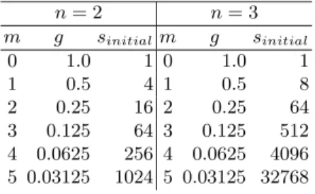
Initial Decomposition. The search domain (or feasible region) of problem (1) is ann-dimensional interval,I, defined by the cartesian product ofnintervals, one per each problem dimension:I=I1×I2×...×In. The PSSA-HeD approach starts by performing anhomogeneous decompositionof these initial intervals.
Each initial interval Ii (i= 1,2, ..., n) is subdivided in 2m subintervals, such that each subinterval has the same relative width or granularityg, as given by
g= 1
2m, withm∈N0 (6)
A subdomain is thus a particular combination of subintervals (with one subin-terval per problem dimension). The overall number of initial subdomains,sinitial, with granularityg, that is generated for ndimension problems is given by
sinitial= 1
g
n
= 2m×n (7)
Table 1.Decomposition granularity and number of initial subdomains.
n= 2 n= 3
m g sinitialm g sinitial
0 1.0 1 0 1.0 1
1 0.5 4 1 0.5 8
2 0.25 16 2 0.25 64
3 0.125 64 3 0.125 512
4 0.0625 256 4 0.0625 4096
5 0.03125 1024 5 0.03125 32768
Recursive Decomposition. With PSSA-HeD, SSA is first applied to the ini-tial (sub)domain(s), and then, if optima are eventually found, child subdomains will be generated around them. Because an optimum may be located anywhere in its hosting (sub)domain, the child subdomains will not only be smaller than their parent (sub)domain, but will also typically vary in width, thus leading to anheterogeneous decomposition. The new child subdomains will, in turn, be searched using SSA and, if optima are found, more subdomains will be gener-ated, until a stop criteria is met. As such, the decomposition is both dynamic and recursive, and the generated subdomains may be seen as part of an expanding search tree where each node/leaf subdomain refines its ancestor.
The stop criteria for this recursive behavior is as follows:
1) if none real optimum is found in a subdomain, then no child subdomains will be generated;
2) otherwise, such generation will take place, but only if the current branch of the search tree has not yet achieved a maximum depth or heighth∈N;
3) all subintervals of a new subdomain must have a minimum distance ofμfrom their parent optimum, or the new subdomain will be ignored.
With regard to the height h, a generic value ofh∈N, means that a search branch may progress as far as h−1 levels bellow the root level. Thus, h = 1 means that the search will be confined to the root of the search tree (in which case PSSA-HeD would be no different than PSSA-HoS). When h = ∞ such means that only criteria 1) and 3) are applied.
In PSSA-HeD, the initial set of homogeneous subdomains is the root of a search tree. If the root is to be defined as the full original domain of the opti-mization function, such is simply achieved withg= 1.0 (orm= 0). The purpose of settingg <1.0 (orm >0), thus starting the search with a grid of homogeneous subdomains, is to increase the probability of finding already several optima in the 1st level of the search tree and thus trigger the generation of many addi-tional new subdomains. Otherwise, withg = 1.0, the number of optima found will typically be very limited and their descendant subdomains will be too few and too large to trigger a sustained recursive search.
slaves. This is advantageous because it inhibits the premature termination of theslaves: there may be times when all available subdomains are being processed byslaves; in this scenario, if an idleslave asked themasterfor a subdomain, it would receive none; but that would not mean that theslavecould terminate once, in the near future, more new unprocessed subdomains might become available, as a byproduct of the current workingslaves; thus, it is better for themasterto push subdomains to theslaves (when they become available), than having the
slavespulling them from themaster(at the risk of none being available). In order to achieve the above behavior, the master manages a work-queue with all subdomains yet to process, and a slave-status-array with the current status (idle/busy) of eachslave. Initially, the work-queue is populated with the starting grid of homogeneous subdomains (or with the single full domain, if such is the case), and allslavesare marked as idle in the slave-status-array.
The distribution of subdomains by theslavesis then just a matter of iterating through the slave-status-array and, for each idleslave, dequeue a subdomain from the work-queue, send it to the slave, and mark the slave as busy. During this iteration, the master may find all slaves to be busy, in which case nothing is removed from the work-queue; it may also find the work-queue to be empty, in which case nothing is assignable to the possible idle slaves; if the work-queue is empty and if all slavesare idle, such means the overall recursive search ended.
After a subdomain distribution round, and assuming the overall search process hasn’t yet finished, the master will block, waiting for a message from some
slave; that message will be empty if the slave found no optima in its assigned subdomain; otherwise, it will carry a set of optima found by the slave (and already filtered by him); in the later case, the optima are added to a global set of solutions that is being assembled by themaster(based on all the contributions of the slaves); the optima are also used to generate new-subdomains that will be added to the work-queue; in any case, the slave is marked as idle in the slave-status-array; the masterthen performs the next distribution round.
4
Filtering Criteria
All PSSA variants produce false minima - some examples are the points in the limits of the subdomains generated. Therefore, filtering criteria are needed to eliminate such false minima. This section presents three criteria, to be used in sequence. In PSSA-HeD they are applied in theslaves, right after running SSA in a subdomain; thus, themasteronly receives sets of validated optima.
Criterion 1
At a given moment, there are a total of ssubdomains (withs≥sinitial). Each subdomainv is defined by nintervals with left and right limits av
i and bvi, res-pectively, for i = 1, ..., n. Consider xv (with coordinatesxv
i, for i = 1, ..., n) a minimum found by at subdomainv. Define the vectordwith componentsdi as
and define Δ1 as
Δ1=
n
i=1
d2
i, withi= 1, ..., n.
Criterion 1 is then defined as follows:
1. Considerǫ1 a positive constant.
2. IfΔ1< ǫ1 thenxv is not a candidate to a minimum of problem (1).
The situation targeted by this criterion is the one in which a subdomain v
doesn’t have minimum values except in its interval limits.
Criterion 2
Consider the unit vector, 1i, with all components null except the component i with unit value. Consider the vectore, with componentei defined as
ei=
f(xv+δ1
i)−f(xv)
δ , fori= 1, ..., n
withδa small positive value. Define alsoΔ2 as
Δ2=
n
i=1
e2 i.
Criterion 2 is thus defined as:
1. Considerxv that satisfy the Criterion 1.
2. IfΔ2> ǫ2 thenxv is not a candidate to a minimum of problem (1).
Criterion 3
Consider the setX∗= xj, j= 1..., n∗
of all solutions that satisfy the Criterion 2 and letn∗be the cardinality of the setX∗.
Criterion 3 is defined as follows:
1. Considerxi∈X∗.
2. The pointxi is a possible minimum value of problem (1) if
xi−xj
> ǫ3, for allj= 1, ..., n∗ andj=i
5
Numerical Results
5.1 Experimental Setup
PSSA-HeD was evaluated in a small commodity cluster of 4 nodes (with one Intel Q9650 3.0GHz quad-core CPU per each node), running Linux ROCKS version 5.4, with the Gnu C Compiler (GCC) version 4.1.2 and MPICH2 version 1.4.
All PSSA executions spawned 16 MPI processes (1masterand 15slaves, one MPI process per cluster core), even if there were a surplus of unused slaves
in certain scenarios. The MPICH2 “machinefile” used was designed to place the first 4 MPI processes (the master and the first 3 slaves) in a single node and scatter (alternately) the remaining 12slaves across the other 3 nodes. This particular configuration maximizes performance both for scenarios with very few subdomains (mostly handled by theslavesof the 1st node without network exchanges), and with lots of subsubdomains (requiringslavesfrom all the nodes, in which case network exchanges benefit from the dispersion of their endpoints). Five problems were evaluated: Ackley, Branin, Griewank, Michalewicz and Shubert [6]. All have more than one local solution, thus suitable to a parallel search of the solutions. Important parameters used wereδ= 5.0 andl = 5 for SSA, andμ= 0.001,ǫ1= 10−4,ǫ2= 10−3andǫ3= 10−2 for PSSA-HeD.
Moreover, in order to know the performance gains introduced by the PSSA-HeD parallel approach, it was also necessary to conduct the optima search by executing SSA in sequence (one subdomain at a time). The set of subdomains searched serially is not exactly the same as the one searched in parallel by PSSA-HeD, once SSA is a stochastic algorithm. However, the overall number of subdo-mains searched (s), and the overall number of optima found (n∗), are similar for
the two approaches, thus making SSA a valid baseline to evaluate PSSA-HeD.
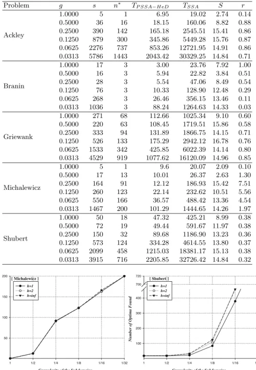
5.2 Experimental Results
The results of the evaluation are presented in Tables 2 to 4, for different values of the recursive search depth:h= 1,h= 2 and h=∞. In the following tables,
– gis the granularity of the initial decomposition,
– sis the overall number of subdomains searched with PSSA-HeD,
– n∗ is the overall number of optima found with PSSA-HeD,
– TP SSA−HeD is the parallel search time (in seconds) with PSSA-HeD,
– TSSAis the sequential search time (in seconds) with SSA,
– S=TSSA/TP SSA−HeD is the speedup of PSSA-HeD against SSA,
– r=n∗/T
P SSA−HeD is the search rate (optima/second) of PSSA-HeD. The tables show that decreasing the decomposition granularity (g) yields, in general, a higher number of optima found (n∗). The only exception is the Branin
Table 2.Experimental results withh= 1
Problem g s n∗ T
P SSA−H eD TSSA S r
Ackley
1.0000 1 1 1.09 1.09 1.00 0.92
0.5000 4 9 7.57 20.16 2.66 1.19
0.2500 16 57 8.23 88.98 10.81 6.93
0.1250 64 233 29.90 363.70 12.16 7.79
0.0625 256 676 98.70 1372.94 13.91 6.85
0.0313 1024 1425 333.57 4975.80 14.92 4.27
Branin
1.0000 1 3 3.66 3.67 1.00 0.82
0.5000 4 3 4.15 11.87 2.86 0.72
0.2500 16 3 5.54 37.75 6.81 0.54
0.1250 64 3 10.30 119.73 11.62 0.29
0.0625 256 3 27.45 347.57 12.66 0.11
0.0313 1024 3 85.32 1256.01 14.72 0.04
Griewank
1.0000 1 18 5.74 5.72 1.00 3.14
0.5000 4 23 5.82 17.15 2.95 3.95
0.2500 16 34 8.93 79.96 8.95 3.81
0.1250 64 69 21.46 251.65 11.73 3.22
0.0625 256 187 58.77 836.70 14.24 3.18
0.0313 1024 576 194.69 2819.53 14.48 2.96
Michalewicz
1.0000 1 1 4.68 4.68 1.00 0.21
0.5000 4 13 6.46 11.58 1.79 2.01
0.2500 16 92 5.81 33.89 5.83 15.83
0.1250 64 123 8.87 79.04 8.91 13.87
0.0625 256 163 22.07 291.38 13.20 7.39
0.0313 1024 200 87.94 1207.94 13.74 2.27
Shubert
1.0000 1 18 14.03 14.02 1.00 1.28
0.5000 4 18 10.53 38.00 3.61 1.71
0.2500 16 22 10.12 121.82 12.04 2.17
0.1250 64 84 38.49 489.16 12.70 2.18
0.0625 256 379 157.71 2276.67 14.38 2.40
0.0313 1024 707 572.49 8657.49 15.12 1.23
(s) also becomes larger with smaller granularities. Moreover, this growth on the number of optima found, and the number of subdomains, is amplified when the maximum search depth,h, increases. Figures 1 and 2 allow to compare, for each problem (except Branin), the values ofn∗ attained with different valuesh.
A conclusion inferred from Figures 1 and 2 is that, in general, increasing the search depth (h) finds more optima, although going from h = 2 to h = ∞
Table 3.Numerical results with withh= 2
Problem g s n∗ T
P SSA−H eD TSSA S r
Ackley
1.0000 5 1 6.92 19.46 2.81 0.14
0.5000 30 15 20.31 160.26 7.89 0.74
0.2500 202 99 89.29 1133.92 12.70 1.11
0.1250 714 294 282.64 4392.66 15.54 1.04
0.0625 2151 739 811.51 12799.00 15.77 0.91
0.0313 5725 1427 2011.74 30152.16 14.99 0.71
Branin
1.0000 17 3 6.53 23.90 3.66 0.46
0.5000 16 3 5.93 22.71 3.83 0.51
0.2500 28 3 5.54 47.06 8.49 0.54
0.1250 76 3 10.05 128.13 12.75 0.30
0.0625 268 3 27.49 365.16 13.28 0.11
0.0313 1036 3 88.51 1269.57 14.34 0.03
Griewank
1.0000 78 24 37.91 385.29 10.16 0.63
0.5000 76 35 32.72 375.71 11.48 1.07
0.2500 116 50 41.95 526.15 12.54 1.19
0.1250 288 106 88.03 1231.37 13.99 1.20
0.0625 955 271 234.04 3484.63 14.89 1.16
0.0313 3249 792 685.68 10012.68 14.60 1.16
Michalewicz
1.0000 5 1 12.55 19.90 1.59 0.08
0.5000 17 13 10.19 26.42 2.59 1.28
0.2500 164 91 12.64 185.29 14.66 7.20
0.1250 260 123 18.76 233.52 12.45 6.56
0.0625 545 163 38.92 488.48 12.55 4.19
0.0313 1465 201 102.53 1442.62 14.07 1.96
Shubert
1.0000 50 18 43.1 396.75 9.21 0.42
0.5000 68 18 47.97 559.17 11.66 0.38
0.2500 110 31 64.98 806.74 12.42 0.48
0.1250 434 108 241.97 3529.14 14.59 0.45
0.0625 1803 467 1031.21 15063.96 14.61 0.45
0.0313 3893 715 2183.50 32507.96 14.89 0.33
Granularity of the Subdomains
1 1/2 1/4 1/8 1/16 1/32
Number of Optima Found
100 200 300 400 500 600 700 1420 1440
h=1 h=2 h=inf
[ Ackley]
Granularity of the Subdomains
1 1/2 1/4 1/8 1/16 1/32
Number of Optima Found 100
200 300 600 800
h=1 h=2 h=inf
[ Griewank ]
Table 4.Experimental results with withh=∞
Problem g s n∗ T
P SSA−H eD TSSA S r
Ackley
1.0000 5 1 6.95 19.02 2.74 0.14
0.5000 36 16 18.15 160.06 8.82 0.88
0.2500 390 142 165.18 2545.51 15.41 0.86
0.1250 879 300 345.86 5449.28 15.76 0.87
0.0625 2276 737 853.26 12721.95 14.91 0.86
0.0313 5786 1443 2043.42 30329.25 14.84 0.71
Branin
1.0000 17 3 3.00 23.76 7.92 1.00
0.5000 16 3 5.94 22.82 3.84 0.51
0.2500 28 3 5.54 47.06 8.49 0.54
0.1250 76 3 10.33 128.90 12.48 0.29
0.0625 268 3 26.46 356.15 13.46 0.11
0.0313 1036 3 88.24 1264.63 14.33 0.03
Griewank
1.0000 271 68 112.66 1025.34 9.10 0.60
0.5000 220 63 108.45 1719.51 15.86 0.58
0.2500 333 94 131.89 1866.75 14.15 0.71
0.1250 526 133 175.29 2942.12 16.78 0.76
0.0625 1533 342 425.85 6022.39 14.14 0.80
0.0313 4529 919 1077.62 16120.09 14.96 0.85
Michalewicz
1.0000 5 1 9.6 20.07 2.09 0.10
0.5000 17 13 10.01 26.37 2.63 1.30
0.2500 164 91 12.12 186.93 15.42 7.51
0.1250 260 123 22.14 232.62 10.51 5.56
0.0625 550 166 36.57 488.42 13.36 4.54
0.0313 1467 200 101.29 1444.65 14.26 1.97
Shubert
1.0000 50 18 47.32 425.21 8.99 0.38
0.5000 72 19 49.44 591.67 11.97 0.38
0.2500 150 32 89.68 1186.90 13.23 0.36
0.1250 573 124 334.28 4614.55 13.80 0.37
0.0625 2099 458 1215.03 18381.17 15.13 0.38
0.0313 3915 716 2205.85 32726.42 14.84 0.32
Granularity of the Subdomains
1 1/2 1/4 1/8 1/16 1/32
Number of Optima Found 50
100 150 200
h=1 h=2 h=inf
[ Michalewicz ]
Granularity of the Subdomains
1 1/2 1/4 1/8 1/16 1/32
Number of Optima Found
100 200 300 400 700 720
h=1 h=2 h=inf
[ Shubert ]
Granularity of the Initial Subdomains
1 1/2 1/4 1/8 1/16 1/32
Search Speedups 0 2 4 6 8 10 12 14 16 ideal h=1 h=2 h=inf
[ Ackley ]
Granularity of the Initial Subdomains
1 1/2 1/4 1/8 1/16 1/32
Search Speedups 0 2 4 6 8 10 12 14 16 ideal h=1 h=2 h=inf
[ Griewank ]
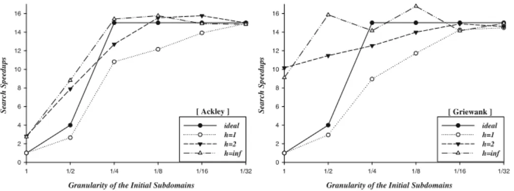
Fig. 3.Search speedups for Ackley and Griewank
Granularity of the Initial Subdomains
1 1/2 1/4 1/8 1/16 1/32
Search Speedups 0 2 4 6 8 10 12 14 16 ideal h=1 h=2 h=inf
[ Michalewicz ]
Granularity of the Initial Subdomains
1 1/2 1/4 1/8 1/16 1/32
Search Speedups 0 2 4 6 8 10 12 14 16 ideal h=1 h=2 h=inf
[ Shubert ]
Fig. 4.Search speedups for Michalewicz and Shubert
With regard to the computational efficiency, the speedups (S) provided by PSSA-HeD against SSA executed serially over the same subdomain set, are not far from ideal values, denoted by Sideal. This may be verified in the graphics from Figures 3 to 4 (again, the Branin function is omitted, for reasons already explained). The way in which the ideal speedupSidealis established is as follows:
– when h = 1, the number of subdomains is static, that is, s = sinitial (as defined in Table 1); it becomes possible to define, a priori, the maximum expected speedup: with 15 MPIslaves,Sidealwill match the number ofslaves actively engaged in optima search; ifs= 1, thenSideal= 1 once only 1 slave will be necessary (the other 14 will remain idle); if s = 4, thenSideal = 4 once only 4 slaves will be needed2; whens≥15, allslaveswill be necessary and the maximum theoretical speedup will beSideal= 15;
2
The same rationale would be valid with s = 8, but the tested functions are all
Granularity of the Subdomains
1 1/2 1/4 1/8 1/16 1/32
Search Rates 0 1 2 3 4 5 6 7 8 h=1 h=2 h=inf
[ Ackley ]
Granularity of the Subdomains
1 1/2 1/4 1/8 1/16 1/32
Search Rates 0,0 0,5 1,0 1,5 2,0 2,5 3,0 3,5 4,0 h=1 h=2 h=inf
[ Griewank ]
Fig. 5.Search rates for Ackley and Griewank (optima/second)
Granularity of the Subdomains
1 1/2 1/4 1/8 1/16 1/32
Search Rates 0 2 4 6 8 10 12 14 16 h=1 h=2 h=inf
[ Michalewicz ]
Granularity of the Subdomains
1 1/2 1/4 1/8 1/16 1/32
Search Rates 0,0 0,5 1,0 1,5 2,0 2,5 h=1 h=2 h=inf
[ Shubert ]
Fig. 6.Search rates for Michalewicz and Shubert (optima/second)
– ifh >0, thens≥sinitial, and so the values 1, 4 and 15 ofSideal withh= 1 are no longer upper bounds for the real speedup; instead, they become a lower bound for the ideal speedup (still, useful as reference for the real speedup).
The proximity between the measured (real) speedups and the theoretical ones (specially with small granularities or, conversely, with many subdomains) proves the merit, performance-wise, of the parallelization approach followed by PSSA-HeD. From a numerical point of view, the main advantage of PSSD-HeD was also already discussed: enabling the efficient finding of many more optima. However, the final decision on which granularity (g) and which search depth (h) to choose depends on the desired balance between i) number of optima found and ii) search time. In this regard, one way to combine both metrics into a single one is through the search rater (optima/second), the last metric shown in the tables. Figures 5 to 6 present the graphics ofr for all functions except Branin.
thenh=∞; b) for each value ofh, each function maximizes the search rate with a different granularity (e.g., withh= 1, Ackley maximizes the rate withg= 1/8, Griewank maximizes with g = 1/2, Michalewicz maximizes with g = 1/4 and Shubert maximizes withg= 1/16); it is thus very difficult (if not impossible) to define a common granularity, that maximizes the search rate for all functions.
5.3 Comparison with PSSA-HoS
As initially stated, the new PSSA-HeD approach builds on a first attempt to parallelize SSA, then named PSSA [20]. This first approach, renamed as PSSA-HoS in the context of this paper, is based on a homogeneous decomposition of the search domain, a decomposition that is in fact identical to the one used in PSSA-HeD whenh= 1; however, while PSSA-HoS performs a static distribution of the initial (and only) subdomain set by the MPI slaves, PSSA-HeD always performs a dynamic distribution irregardless of the parameter h. Although no detailed results are here supplied, PSSA-HoS was also executed under the same experimental conditions in which PSSA-HeD was evaluated. The conclusion was that the dynamic distribution performed by PSSA-HeD achieves better load balancing, providing to PSSA-HeD (withh= 1) marginally better search times (≈10%, on average) than PSSA-HoS (the number of optima found is similar).
6
Conclusions and Future Work
This work expands previous investigation on the parallelization of the SSA stochastic algorithm, aimed at finding all local solutions of multimodal objec-tive function problems. The computation experiments conducted showed that the new PSSE-HeD approach is capable of locating a large number of local optima, improving on the numerical efficiency of the previous PSSA-HoS ap-proach. Moreover, PSSE-HeD may be tunned to achieve the desired compromise between search time and number of optima found. The speedups achieved by the new parallel code are also close to the experimental testbed ideal levels.
In the future, we intend to further refine PSSA and apply it to solve more complex constrained multilocal optimization problems.
Acknowledgments. This work was been supported by FCT (Funda¸c˜ao para a Ciˆencia e Tecnologia) in the scope of the project PEst-OE/EEI/UI0319/2014.
References
1. Chelouah, R., Siarry, P.: A continuous genetic algorithm designed for the global optimization of multimodal functions. Journal of Heuristics 6, 191–213 (2000) 2. Eriksson, P., Arora, J.: A comparison of global optimization algorithms applied to
3. Floudas, C.: Recent advances in global optimization for process synthesis, design and control: enclosure of all solutions. Computers and Chemical Engineering, 963– 973 (1999)
4. The GNU C Library,http://www.gnu.org/software/libc/manual/.
5. Guibas, L.J., Sedgewick, R.: A Dichromatic Framework for Balanced Trees. In: Proceedings of the 19th Annual Symposium on Foundations of Computer Science, pp. 8–21 (1978)
6. Hedar, A.R.: Global Optimization Test Problems,
http://www-optima.amp.i.kyoto-u.ac.jp/member/student/hedar/ Hedar files/TestGO.htm
7. High-Performance Portable MPI,http://www.mpich.org/
8. Ingber, L.: Very fast simulated re-annealing. Mathematical and Computer Mod-elling 12, 967–973 (1989)
9. Kernighan, Ritchie, D.M.: The C Programming Language, 2nd edn. Prentice Hall, Englewood Cliffs (1988) ISBN 0-13-110362-8
10. Kiseleva, E., Stepanchuk, T.: On the efficiency of a global non-differentiable op-timization algorithm based on the method of optimal set partitioning. Journal of Global Optimization 25, 209–235 (2003)
11. Le´on, T., Sanmat´ıas, S., Vercher, H.: A multi-local optimization algorithm.
Top 6(1), 1–18 (1998)
12. Message Passing Interface Forum,http://www.mpi-forum.org/
13. Parsopoulos, K., Plagianakos, V., Magoulas, G., Vrahatis, M.: Objective function stretching to alleviate convergence to local minima. Nonlinear Analysis 47, 3419– 3424 (2001)
14. Parsopoulos, K., Vrahatis, M.: Recent approaches to global optimization problems through particle swarm optimization. Natural Computing 1, 235–306 (2002) 15. Pereira, A.I., Fernandes, E.M.G.P.: A reduction method for semi-infinite
program-ming by means of a global stochastic approach. Optimization 58, 713–726 (2009) 16. Pereira, A.I., Fernandes, E.M.G.P.: Constrained Multi-global Optimization
us-ing a Penalty Stretched Simulated Annealus-ing Framework. In: Numerical Analysis and Applied Mathematics, AIP Conference Proceedings, vol. 1168, pp. 1354–1357 (2009)
17. Pereira, A.I., Fernandes, E.M.G.P.: Comparative Study of Penalty Simulated An-nealing Methods for Multiglobal Programming. In: 2nd International Conference on Engineering Optimization (2010)
18. Pereira, A.I., Ferreira, O., Pinho, S.P., Fernandes, E.M.G.P.: Multilocal Program-ming and Applications. In: Zelinka, I., Snasel, V., Abraham, A. (eds.) Handbook of Optimization. Intelligent Systems Series, pp. 157–186. Springer (2013)
19. Price, C.J., Coope, I.D.: Numerical experiments in semi-infinite programming. Computational Optimization and Applications 6, 169–189 (1996)
20. Ribeiro, T., Rufino, J., Pereira, A.I.: PSSA: Parallel Stretched Simulated Anneal-ing. In: Numerical Analysis and Applied Mathematics, AIP Conference Proceed-ings, vol. 1389, pp. 783–786 (2011)
21. Salhi, S., Queen, N.: A Hybrid Algorithm for Identifying Global and Local Minima When Optimizing Functions with Many Minima. European Journal of Operations Research 155, 51–67 (2004)
22. Tsoulos, I., Lagaris, I.: Gradient-controlled, typical-distance clustering for global
optimization (2004),http://www.optimization.org