Bundled Discounts: Strategic Substitutes or
Complements?
Duarte Brito
yUniversidade Nova de Lisboa and CEFAGE-UE
Helder Vasconcelos
zFaculdade de Economia, Universidade do Porto, CEF.UP and CEPR
June 2, 2014
Abstract
Bundled discounts by pairs of otherwise independent …rms play an increasingly impor-tant role as a strategic tool in several industries. Given that prices of …rms competing for the same consumers are strategic complements, one would expect their discounts levels also to be strategic complements. However, in this paper we show that under some cir-cumstances bundled discounts may be strategic substitutes. This occurs under vertically di¤erentiated products where a low quality pair of producers may indeed prefer to lower its discount after an increase in the discount o¤ered by a high quality pair of producers. Keywords: Bundled Discounts, Bilateral Bundling, Strategic Substitutes.
JEL Classi…cation: D43; L13; L41.
This paper was …nanced by national funds from the FCT under project PTDC/EGE-ECO/111558/2009.
yDCSA, Faculdade de Ciências e Tecnologia da Universidade Nova de Lisboa, Quinta da Torre, 2829-516
Caparica, Portugal. E-mail: dmb@fct.unl.pt.
zFaculdade de Economia da Universidade do Porto, Rua Dr. Roberto Frias, 4200-464 Porto, Portugal.
1
Introduction
When prices are strategic complements, as is commonly accepted in the literature, one would
expect that the best response of a given …rm to an increase in a discount o¤ered by a rival
would be to increase its discount as well. In general, common wisdom holds that “[w]hether
the competitive action is based on price, comparison advertising or coupons, a more aggressive
competitive action or commitment will likely lead to a more aggressive response, and vice
versa.” (Sengul et al (2012)). This implies that discounts are generally accepted as strategic
complements.1 This paper investigates whether this conventional wisdom holds good in the
context of discounts o¤ered to consumers who purchase bundles in which each component good
is sold by a di¤erent and independent …rm.
Bundled discounts have recently become very common: examples range from discounts in
the electricity bill in the form of vouchers one can redeem at supermarket chains, o¤erings of
cinema or amusement park tickets at gas stations or fast food chains, restaurant discounts for
guests at a given hotel, car-rental discount for passengers of a given airline, and discounts for
drug cocktails made up of components produced by di¤erent …rms, to name just a few.
Bundled discounts by independent producers were studied by Gans and King (2006) and
Brito and Vasconcelos (2014), under horizontal and vertical di¤erentiation, respectively. These
discounts have several implications: (i) if set in advance, discounts may work as commitment devices; (ii) at the time they are set, the relevant objective function (joint pro…t) is di¤erent
from the one that is relevant for price setting in the ensuing stage (individual pro…t); and (iii)
the discount is typically …nanced by more than one …rm.
Contrary to common wisdom, we …nd that bundled discounts may be strategic substitutes
rather than complements: under some circumstances, the best-response to an increase in the
rivals’ discount may be for a pair of …rms to reduce its own discount. This possibility result is
illustrated within a theoretical framework based on a simpli…ed version of Brito and Vasconcelos
(2014).
Section 2 provides a brief description of the model. Section3 presents the result. Finally, Section 4concludes. All expressions are presented in the appendix.
1The strategic complement/strategic substitute distinction was introduced in the literature by Bulow et al
2
The model
We consider a two-product version of Gabszewicz and Thisse (1979), where each product
is sold both by a high and also by a low quality …rm. Let AX and AY be the high quality
sellers of products X and Y, respectively, and let BX and BY denote the corresponding low
quality producers. In addition, let Pj and pj denote the headline prices set by Aj and Bj,
respectively, with j =X; Y. We assume that …rm AX is allied with AY and that …rm BX is
allied with BY, meaning that a pair of allied …rms o¤ering products of similar quality level will
o¤er a discount to those consumers who purchase both products from them. Given that there
is symmetry between allied …rms, we assume that they will equally …nance the discount.2 The
discount o¤ered by the high (resp. low) quality producers is denoted by A (resp. B).
The timing of the game is as follows. At a …rst stage, the pairs of allied …rms decide
simultaneously upon the discount that maximizes their joint pro…ts. Afterwards, the four
…rms set their headline prices simultaneously so as to maximize individual pro…t.3
Consumers are assumed to always purchase one unit of each product. Moreover, consumers
are uniformly distributed on a unit square where each axis measures consumers’ valuation for
quality of each product. A consumer with valuations for quality X; Y on [0;1]2 purchases
from AX and AY if and only if:
Ys > PY A pY
Xs > PX A pX
Ys+ Xs > PX +PY A (pX +pY B)
wheresrepresents the di¤erence between the high and the low quality versions of each product,
which is assumed to be equal. The …rst and second inequalities ensure that, given that the
consumer selects the high quality version of one of the products, it will also prefer the high
quality version of the other product, because the valuation for the increment in quality more
than compensates for any increase in price. The third inequality, on the other hand, ensures
that the high quality pair of products generates more surplus than the low quality pair.
The demand for each of the four possible combinations of products is given by the number
of consumers that verify the three relevant inequalities. We write QAB to denote the number
2We consider bundling by …rms with the same quality to be the “natural” scenario. A high quality producer
would probably not be interested in being allied with a low quality one as this would likely a¤ect its reputation. Further, considering only this scenario also allows us to avoid having to determine the optimal way of sharing the discount in an asymmetric alliance involving a high quality and a low quality producer.
of consumers that purchase product X from …rm A and product Y from …rmB, and likewise
for the three remaining possible combinations.4
Discounts are assumed to be small. We de…ne a small discount as a discount such that the
four possible combinations of products have a positive market share for all discount levels of
the competitors (if any), at the equilibrium prices. Formally, we assume that( A; B)2[0; ]2,
where is presented in the appendix.5 To some extent, small discounts can be justi…ed by
the management literature that has highlighted the ine¤ectiveness of high discounts. Raghubir
(1998) and (2004), Barat and Paswan (2005) or Wu et al. (2011) point out the possibility that
a high discount may trigger negative consumer deductions about the headline price or quality,
or even create negative emotions due to the implicit price discrimination involving coupons.
Moreover, small discounts are empirically more relevant, as most observed discounts would
most probably fall within our de…nition of “small discount”.6
The equilibrium is obtained by working backwards. For a given pair of discounts, the
(individual) pro…t maximizing prices are obtained. Then, discounts which maximize joint
pro…ts are characterized.
3
Result
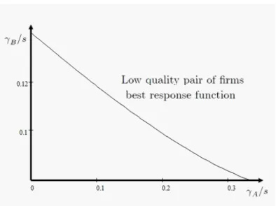
Figure1 presents the best-response function for the pair of low quality …rms. We can only
characterize this function numerically and it has a downward slope: discounts are strategic
substitutes.7
To understand why the low quality …rms may prefer to lower their discount when rivals
increase theirs, one needs to understand how the discount impacts the allied …rms’ joint pro…t
and how this impact changes with the rivals’ discount level.
Using i := is, joint pro…t for the low quality …rms is
B =pY(QBB+QAB) +pX(QBB+QBA) BsQBB:
Due to the fact that the equilibrium prices of both products of similar quality are symmetric,
B may be written as
B = 2pX(QBB+QAB) BsQBB: 4The appendix presents the demand functions in detail.
5This is a common assumption in the literature. See Aydemir (2009) or Gans and King (2006).
6In our setting, the upper bound on the discount levels, , represents60%and120%of the headline prices of
the high and low quality component products of the bundle (in the no-discounting benchmark case), respectively.
7It can be showed that the derivative of the high quality pair of …rms joint pro…ts with respect to its discount
Figure 1: Low quality pair of …rms best response function
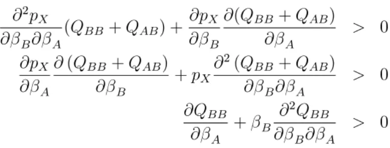
The …rst-order condition in B is8
2 @pX
@ B(QBB+QAB) +pX
@(QBB+QAB)
@ B =s QBB + B @QBB
@ B : (1)
Notice that all derivatives in (1) are positive: the headline price, the number of units entitled
to the discount and the low quality …rms’ aggregate sales increase in B. Price pX increases
with B for two reasons: (i) a higher discount o¤ered by the low quality producers increases
the demand for each low quality product; and (ii) the introduction of the discount can be
interpreted as a unit cost, partially incurred by each …rm, for the units entitled to the discount.
Further, despite the fact that pX increases with the discount, the “net” bundle price decreases
with it, leading to a higher demand for the bundle and also for all low quality products.
The left-hand side in (1) is the discount’s marginal bene…t. As the headline price will
increase (@pX
@ B > 0), the margin per unit is higher, excluding the discount “cost”. Total sales
will also increase (@(QBB+QAB)
@ B > 0). Hence, the discount’s marginal bene…t comes from both
an increase in price and in sales.
The right-hand side in (1) is the discount’s marginal cost. It also includes two e¤ects: (i)
all units that were previously sold as a bundle (QBB) now entitle the corresponding consumers
to a higher discount; and (ii) there will be an increase in the sales entitled to the discount (@QBB
@ B >0).
The optimal discount is obtained when the marginal revenue equals marginal cost. Now, to
understand how allied …rms should react to di¤erent rival’s discounts we need to establish how
marginal bene…t and cost change with A. Di¤erentiating (1) with respect to A we obtain:
2 @
2p
X
@ B@ A
(QBB+QAB) +
@pX
@ B
@(QBB+QAB)
@ A
+pX
@2(Q
BB+QAB)
@ B@ A
+@pX
@ A
@(QBB+QAB)
@ B
s @QBB @ A + B
@2QBB
@ B@ A
Consider …rst the impact of the rivals’ discount on marginal bene…t. The headline price
increases more with own discount in the presence of the rivals’ discount, but this increase
impacts a smaller number of original units demanded. Additionally, although the number of
additional units demanded is now higher, these may be sold at a lower or higher price than in
the absence of a rival discount. Despite the fact that the net result is potentially ambiguous,
the positive e¤ects dominate, implying that there is an incentive to increase own discount when
rivals increase theirs.
As for the marginal cost, when rivals increase the discountQBB becomes larger. However,
fewer additional units will be sold by the low quality pair of …rms as a result of a higher discount.
Although the net e¤ect is again potentially ambiguous, the aggregate e¤ect is positive.
The following table summarizes these e¤ects and also highlights how they change with A.
Marginal Bene…t Marginal Cost
Term: 1st 2nd 1st 2nd
@pX
@ B (QBB+QAB) pX
@(QBB+QAB)
@ B QBB B
@QBB @ B
Sign of derivative wrt A >0 <0 ? >0 >0 <0
| {z } | {z } | {z }
>0 >0 >0
Hence, if discounts are strategic substitutes, it must be that the increase in marginal cost
dominates the increase in marginal bene…t. Perhaps counter-intuitively, when the high quality
rivals’ increase their discount, the sales of the low quality bundle increase: increasing the high
quality bundle discount, increases the high quality headline prices, leading some consumers
who were purchasing products of di¤erent qualities to switch to the low quality bundle. This
then makes it more expensive to increase the low quality bundle discount, as the number of
consumers entitled to it becomes larger.9
9Notice that the impact of the discount on headline prices would not exist if discounts and prices were set
4
Conclusions
Bundled discounts play an increasingly important role as a strategic tool. In many instances,
the discounts are given by pairs of independent …rms who agree to cut prices charged to
consumers who purchase from both of them. Given that prices of …rms competing for the
same consumers are strategic complements, one would expect these discounts to be strategic
complements as well. However, in some circumstances, they may be strategic substitutes.
In this paper, we analyze the case of competition between independent vertically
di¤erenti-ated producers o¤ering bundled discounts. We …nd that the low quality pair of producers may
prefer to lower their discount after an increase in the discount o¤ered by the high quality
pro-ducers. The reason is that the demand for their bundle may actually increase with the rivals’
discount, making their own discount very expensive. As the high quality discount increases,
so will the corresponding headline prices. This means that consumers who were previously
purchasing products of di¤erent quality may prefer to switch to the low quality bundle and
bene…t from the associated discount. In response, this may lead the latter pair of producers to
prefer to decrease their discount.
References
[1] Aydemir, R., (2009), “Essays on Bundling and Low Cost Air Carrier Pricing”,
Ph.D. Dissertation, The University of Texas at Austin, Available for download at:
http://repositories.lib.utexas.edu/bitstream/handle/2152/11639/aydemirr61006.pdf?sequence=2
[2] Barat, S. and A. K. Paswan, (2005) "Do higher face-value coupons cost more than they are
worth in increased sales?", Journal of Product & Brand Management, Vol. 14 (6), pp.379
- 386.
[3] Brito, D. and H. Vasconcelos (forthcoming),“Inter-…rm Bundling and Vertical Product
Di¤erentiation” Scandinavian Journal of Economics.
[4] J. Bulow, J. Geanakoplos, and P. Klemperer (1985), “Multimarket oligopoly: strategic
substitutes and strategic complements”. Journal of Political Economy 93, 488-511,
[5] Gabszewicz, J. and Thisse, J.-F. (1979), “Price Competition, Quality and Income
Dispar-ities”, Journal of Economic Theory 20, 340-359.
[6] Gans, J. and King, S. (2006), “Paying for Loyalty: Product Bundling in Oligopoly”,
[7] Raghubir, P. (1998) "Coupon Value: a Signal for Price?",Journal of Marketing Research,
Vol. 35 (3), pp. 316-324.
[8] Raghubir, P. (2004) "Coupons in context: discounting prices or decreasing pro…ts?",
Jour-nal of Retailing, Vol. 80, pp. 1–12.
[9] Sengul, M., J. Gimeno and J. Dial (2012), “Strategic Delegation : A Review, Theoretical
Integration, and Research Agenda”, Journal of Management, 38(1), 375-414.
[10] Wu, C.-C, Yi-Fen Liu, Ying-Ju Chen, Chih-Jen Wang, (2011) "Consumer responses to
price discrimination: Discriminating bases, inequality status, and information disclosure
timing in‡uences", Journal of Business Research, available online
Appendix
Demand Functions
With no discounts, consumers purchase product i=X; Y from …rm Ai if and only if
V + isA Pi > V + isB pi , i > i :=
Pi pi
s
where V is the reservation price.
Assume the high quality …rms introduce discount A: Then, a consumer characterized by:
X > X =
PX pX
s and Y > Y = PY pY
s will still purchase from AX; AY:
X > X =
PX pX
s and Y < Y = PY pY
s will purchase AX; AY if
XsA PX + YsA PY + A> XsA PX + YsB pY , Y > Ya:=
PY pY A
s :
X < X =
PX pX
s and Y < Y = PY pY
s will purchase AX; AY if
XsA PX+ YsA PY+ A> XsB pX+ YsB pY , X >
PX pX +PY pY A
s Y:
X < X =
PX pX
s and Y > Y = PY pY
s will purchase AX; AY if
XsA PX + YsA PY + A > XsB pX + YsA PY , X > Xa =
PX pX A
s :
Assume additionally that the low quality …rms introduce discount B: Then, a consumer
X < Xa and Y > Y will purchase BX; BY if
XsB pX + YsB pY + B > XsB pX + YsA PY , Y < Yb :=
PY pY + B
s :
X > X and Y < Ya will purchase BX; BY if
XsB pX + YsB pY + B > XsA PX + YsB pY , X < Xb :=
PX pX + B
s :
X > Xa and Y > Ya and X > PX pX+PsY pY A Y will purchase BX; BY if
XsB pX + YsB pY + B > XsA PX + YsA PY + A,
X <
PX pX +PY pY + B A
s Y =
a X +
b Y Y:
Demand functions, resulting from the relevant areas in the( X; Y) space, are:
QAX;BY = 1
PX pX + B
s
PY pY A
s ;
QBX;AY = 1
PY pY + B
s
PX pX A
s ;
QAX;AY = 1
PY pY A
s 1
PX pX A
s
( A+ B)
2
2s2 ;
QBX;BY =
PY pY + B
s
PX pX + B
s
( A+ B)
2
2s2 :
The pro…t functions at the pricing stage are:
X = PX(QAXBY +QAXAY) A
2 (QAXAY)
Y = PY (QAXAY +QBXAY) A
2 (QAXAY)
X = pX(QBXBY +QBXAY) B
2 (QBXBY)
Y = pY (QBXBY +QAXBY) B
2 (QBXBY)
Using i := is and solving the system of …rst-order-conditions one obtains:
PX =
12 A+ 6 B+ 6
2
A+
3
A+
3
B+ 5 A B+ 4 A
2
B+ 4
2
A B+ 8
2 (5 A+ 5 B+ 6)
s
PY =
12 A+ 6 B+ 6 2A+ 3A+ B3 + 5 A B+ 4 A 2B+ 4 2A B+ 8
2 (5 A+ 5 B+ 6) s
pX =
2 A+ 6 B+ 3A+ 6
2
B+
3
B+ 5 A B+ 4 A 2B+ 4
2
A B+ 4
2 (5 A+ 5 B+ 6)
s
pY =
2 A+ 6 B+
3
A+ 6
2
B+
3
B+ 5 A B+ 4 A
2
B+ 4
2
A B+ 4
2 (5 A+ 5 B+ 6)
and
QAX;BY = B
+ 5 A B+ 3 2A+ 2 2B 4 A+ 5 A B+ 2 2A+ 3 2B 2 (5 A+ 5 B+ 6)
2 ;
QBX;AY =
B+ 5 A B+ 3 2A+ 2 2B 4 A+ 5 A B+ 2 2A+ 3 2B 2
(5 A+ 5 B+ 6)
2 ;
QAX;AY =
0
@ 96 A+ 80 B+ 128 A B+ 68 2
A 12
3
A+ 62
2
B 17
4
A 7
4
B
8 A 2B 20 2A B 40 A B3 60 3A B 76 2A 2B+ 32
1
A
2 (5 A+ 5 B+ 6)
2 ;
QBX;BY =
0
@ 40 A+ 48 B+ 88 A B+ 38
2
A+ 52 2B 7 4A 12 3B 17 4B
20 A 2B 8
2
A B 60 A 3B 40
3
A B 76 2A
2
B+ 8
1
A
2 (5 A+ 5 B+ 6)
2 :
For all segments of demand to be positive, one needs to assume that:
4 5 A B 3 2A 2
2
B B 0 (2)
2 5 A B 3 2B 2 2A A 0 (3)
where (3) implies (2). Assuming that both discounts cannot exceed = s , it follows that
Comparative Statics
The derivatives referred in Section3 are:10
@(QBX;BY +QAX;BY)
@ A
= 6 A B 5 B+ 9
2
A+ 5
3
A 3
2
B+ 5 A
2
B+ 10
2
A B 4
(5 A+ 5 B+ 6)
2 <0
@(QBX;BY +QAX;BY)
@ B =
5 A 6 A B+ 3 2A 9 2B 5 3B 10 A 2B 5 2A B+ 2
(5 A+ 5 B+ 6)
2 >0
@2(Q
BX;BY +QAX;BY)
@ B@ A
=
0
@ 108 A+ 86 B+ 180 A B+ 90
2
A+ 25
3
A+ 90
2
B+ 25
3
B
+75 A
2
B+ 75
2
A B+ 40
1
A
(5 A+ 5 B+ 6)
3 >0
@QBX;BY
@ B = 0 B B @
184 A+ 192 B 80 A B+ 6 2A 140 3A 108 2B
65 4A 234 3B 85 4B 630 A 2B 536
2
A B 320 A 3B
280 3A B 450
2
A
2
B+ 104
1
C C A
(5 A+ 5 B+ 6)
3 >0
@QBX;BY
@ A = 0 B B @
128 A+ 124 B 78 A B 84 A3 100 2B 35 4A 170 3B
65 4B 446 A 2B 360 A2 B 230 A 3B 170 3A B
300 2A 2B+ 80
1
C C A
(5 A+ 5 B+ 6)
3 >0
@2QBX;BY
@ A@ B =
1768 A 2440 B 5572 A B 2550
2
A 1560
3
A
2560 2B 325 4A 1560 3B 325 4B 4460 A 2B 4460 2A B
1300 A 3B 1300 3A B 1950 2A 2B 456
(5 A+ 5 B+ 6)
4 <0
and
@PX
@ A =
72 A+ 60 B+ 108 A B+ 48 2A+ 10
3
A+ 49
2
B+ 15
3
B+ 40 A 2B+ 35
2
A B+ 32
2 (5 A+ 5 B+ 6)
2 s >0
@pX
@ B
= 50 A+ 72 B+ 108 A B+ 49
2
A+ 15 3A+ 48 2B+ 10 B3 + 35 A 2B+ 40 2A B+ 16
2 (5 A+ 5 B+ 6)2 s >0
@pX
@ A =
10 B+ 48 A B+ 18 2A+ 10
3
A+ 19
2
B+ 15
3
B+ 40 A 2B+ 35
2
A B 8
2 (5 A+ 5 B+ 6)
2 s <>0
@2p
X
@ B@ A
=
0
@ 338 A+ 178 B+ 430 A B+ 270 2
A+ 75
3
A+
270 2B+ 75 3B+ 225 A 2B+ 225 2A B+ 140
1
A
2 (5 A+ 5 B+ 6)3 >0
Moreover,
@2p
X
@ B@ A
(QBB+QAB) +
@pX
@ B
@(QBB+QAB)
@ A
> 0
@pX
@ A
@(QBB+QAB)
@ B
+pX
@2(QBB+QAB)
@ B@ A
> 0
@QBB
@ A + B
@2QBB
@ B@ A > 0
At the discount stage, the objective function is
B = X + Y =pX(QBXBY +QBXAY) +pY (QBXBY +QAXBY) B(QBXBY)
The …rst-order-conditions are:
@ B
@ B =
0
B B B B B B B B @
20 6B 5B(105 A 129) 4B 195 2A 615 A 430
3
B 140
3
A 1197
2
A 1526 A 100
2
B 504 1836
2
A 1155
3
A 120 A
B 528 A 32 2A 872 3A 534 4A 45 5A+ 160
88 2A+ 132 4A+ 90 5A+ 15 6A+ 32
1
C C C C C C C C A
s
2 (5 A+ 5 B+ 6)
= 0