Rita Mafalda Dionísio de Sousa

(1)

Rita Mafalda Dionísio de Sousa

Mestrado em Economia e Política da Energia e do Ambiente Licenciatura em Economia

Carbon Prices

Dynamic analysis of

European and Californian markets

Dissertação para obtenção do Grau de Doutor em

Alterações Climáticas e Políticas de Desenvolvimento Sustentável

Orientador:

Professor Doutor Rui Santos,

Professor Associado,

Universidade Nova de Lisboa

Co-Orientador: Professor Doutor Luís Aguiar-Conraria,

Professor Associado com Agregação

Universidade do Minho

Júri:

Presidente: Profª. Doutora Maria Paula Pires dos Santos Diogo Arguentes: Prof. Doutor Miguel Pedro Brito St. Aubyn

Prof. Doutor Tiago Morais Delgado Domingos Vogais: Prof. Doutora Maria Isabel Rebelo Teixeira Soares Prof. Doutora Maria Júlia Fonseca de Seixas

Prof. Doutor Rui Jorge Fernandes Ferreira dos Santos Prof. Doutor Luís Francisco Gomes Dias de Aguiar Conraria

(2)

(3)

Copyright

“Carbon Prices - Dynamic analysis of European and Californian Markets”

Rita Mafalda Dionísio de Sousa

Faculdade de Ciências e Tecnologia e a Universidade Nova de Lisboa

A Faculdade de Ciências e Tecnologia e a Universidade Nova de Lisboa têm o direito, perpétuo

e sem limites geográficos, de arquivar e publicar esta dissertação através de exemplares

impres-sos reproduzidos em papel ou de forma digital, ou por qualquer outro meio conhecido ou que

venha a ser inventado, e de a divulgar através de repositórios científicos e de admitir a sua cópia

e distribuição com objectivos educacionais ou de investigação, não comerciais, desde que seja

dado crédito ao autor e editor.

Faculdade de Ciências e Tecnologia, Universidade Nova de Lisboa, 05/05/2014

(4)

(5)

Dedicatory

For Júlia

Acknowledgments

The work presented in this thesis would not be possible without the help of the following people, to whom I am truly grateful.

My supervisors, Professor Rui Santos and Professor Luís Aguiar Conraria. Professor Rui Santos for all the help and support in carrying out the work, for his constructive criticism, and for all the help in meeting the imposed deadlines. I also thank Professor Luís Aguiar Conraria who was the technical pillar of this thesis, sharing knowledge and demonstrating seemingly endless doses of motivation.

Pedro M. Barata, for inspiring the theme I have chosen, and being my mentor. Someone who, despite the short time he has, was available for sharing very helpful comments. The affection he has on climate change issues contaminates all those around him, and I'm no exception.

Professor Isabel Soares, for her manifested interest and curiosity, being the first supporter and supervisor of my academic research on carbon prices.

Relatives, friends and colleagues who helped me when it seemed I had reached a dead end, supporting the revision of the text or making illuminating comments: Isabel Tarroso, Maria João Martins, Nuno Antunes, Ana Rovisco, Renato Rosa, Rui Ochôa, Cláudia Sousa and Professor Mª Joana Soares.

To Nelson Soares and Professor Cláudio Monteiro, at Smartwatt, for their enthusiasm at the start of my academic career and the backing when attending the PhD Lisbon classes.

Professors Jorge Pereira and Peças Lopes, at the Power Systems Unit of INESC Porto, for the support to the 1st year of PhD classes.

I also thank the School of Economics and Management at the University of Minho, for the logistic support, providing me with a workplace, hardware and software.

The promoters of the Doctoral Program in Climate Change and Sustainable Development Poli-cies, for the opportunity to attend advanced studies in this area of reference, in Portugal.

Globally, I thank the people and institutions that facilitated access to essential data to my work: Euronatura, Kate Jazgara at The ICE - IntercontinentalExchange, the European Energy Exchange EEX, the Climate Policy Initiative, the European Climate Assessment and Dataset, and Michelle Breckner at the Western Regional Climate Center US.

Finally, I thank my Mother, for the relentless support with Júlia and everything else. Without her it would not have been possible to complete this work. And that sums it up.

My Father, another huge support, irrefutable proof that many miles do not necessarily make great distances.

Júlia, for the eternal smiles she was born with, and with which she presents me with every day. And Marco, for the Art that he puts in my life every day. It is what gives everything a meaning.

(6)

(7)

Resumo

Os mercados de carbono existem para promover a redução de emissões de gases com efeito de

estufa onde esta é mais custo-eficiente. O preço do bem transaccionável, o carbono (CO2

equi-valente), é, por isso, uma variável chave nas decisões de gestão da produção e do risco nos

mer-cados associados a actividades ligadas à queima de combustíveis fósseis, como a produção de

electricidade.

Este trabalho pretende melhorar a análise da dinâmica dos preços de carbono, considerando a

possibilidade de existência de efeitos multidireccionais entre preços de carbono, da energia

(fi-nal e primária), de licenças de offsets, e a performance da economia, em várias frequências. As

duas principais perguntas de investigação são: (i) o que orienta os preços de carbono? (ii) em

que preços as variações são consequência dos preços de carbono? Utilizaram-se duas

metodo-logias complementares: (a) um modelo vector auto-regressivo (de uso comum na

macroecono-mia e mercados financeiros, mas pouco aplicado à relação energia-carbono) que permite a

aná-lise de causalidade e de impulso-resposta de preços diários; e (b) uma inovadora anáaná-lise

multi-variada de wavelets, que permite perceber a relação e causalidade existente entre as variáveis

nas dimensões tempo e frequência, nomeadamente em ciclos mais longos (4~8 e 8~20 meses),

não captada em nenhuma análise prévia. Consideram-se como casos de estudo os mercados de

carbono Europeu (EU ETS) e da Califórnia (AB32), sendo este o primeiro trabalho de investigação

a apresentar a análise do mercado americano. A análise abrange o período de 2008 a 2013, e

excluiu a fase I do EU ETS, para maior consistência da amostra.

Os resultados obtidos permitem sugerir que a economia e os preços da electricidade orientam

o preço de carbono Europeu, enquanto na Califórnia o gás e o petróleo têm um papel mais

re-levante, havendo, portanto maior influência dos preços de energia final no mercado mais

ma-duro. Também observamos que o preço das CERs não influencia o preço de carbono Europeu.

Inversamente, este estudo apresenta pela primeira vez evidências de que os preços do carbono

têm impactos no preço da electricidade em ciclos mais longos (8~20 meses) e no carvão em

ciclos curtos, e com duração limitada aos primeiros dias. Sugere, portanto, que o mercado de

emissões surte efeitos mais significativos em ciclos mais longos. Por fim, o preço de carbono

Europeu também mostra influências nos preços das CERs. Os resultados obtidos são

estatistica-mente significativos e relevantes, e irão melhorar a qualidade na tomada de decisão das partes

envolvidas nos mercados de energia e de carbono, poluidores e reguladores.

(8)

(9)

Abstract

Carbon markets’ goal is to promote the reduction of emissions of greenhouse gases where it is most cost-efficient. This makes the price of the tradable good – carbon dioxide equivalent (CO2e) - a key variable in management and risk decisions, in markets related to activities connected

with the burning of fossil fuels, such as power generation.

This work aims to improve the analysis of carbon prices’ dynamics, considering the possibility of multidirectional effects between prices of CO2e, energy (primary and final), offsets licenses and

the economy performance, in various frequencies. The two main research questions are: (i) what

drives carbon price variations? (ii) what variations do carbon prices drive? We used two

comple-mentary methodologies: (a) a vector autoregression model (of common use in macroeconomics

and financial markets but not in carbon-energy relations), which allows the analysis of causality

and of impulse-response functions of daily prices; and (b) an innovative multivariate wavelet

analysis, which allows us to understand the relationship and causal link between the variables

in the time and frequency dimensions, particularly in longer cycles (4~8 and 8~20 months), not

perceived in previous studies. As case studies we considered the European (EU ETS) and

Califor-nia (AB32) carbon markets. This is the first research to present the analysis of the referred US

market. The analysis covers the 2008-2013 period, intentionally excluding the EU ETS phase I,

for greater consistency of results.

Results suggest that the economy and electricity drive the price of European carbon, while gas

and oil have a greater role in California. So, there is a greater influence of final energy prices in

the most mature market. We also observe that the price of CERs does not affect the European

carbon price. On the other hand, this study shows for the first time that carbon prices have

impacts on electricity prices over longer cycles (8~20 months) and in coal over short cycles

(lim-ited to the first days). It is suggested that the carbon market has more significant effects in longer

cycles. The price of European carbon also has impact in CERs prices. The results are statistically

significant and relevant, and will improve the quality of decision making of all parties involved

in the energy and carbon markets - polluters and regulators included.

(10)

(11)

INDEX OF FIGURES

Figure 1 : Emission trading schemes around the World ... 5

Figure 2 : Sea surface temperatures averaged over the NINO3 area in the eastern Pacific. ... 23

Figure 3 : The Fourier transform of a time series ... 24

Figure 4 : Wavelet power spectrum of sea surface temperatures in the eastern Pacific ... 26

Figure 5 : The real part of a Morlet wavelet ... 31

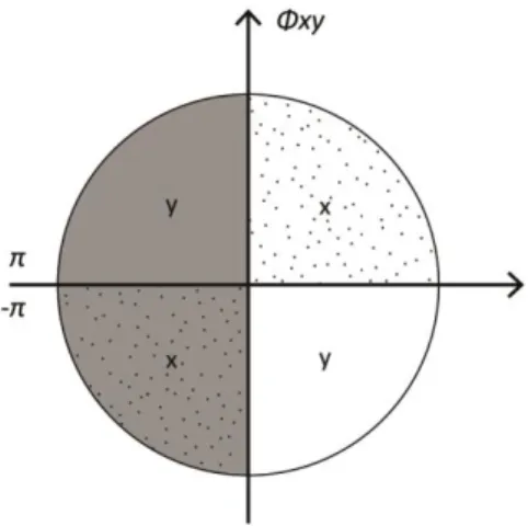
Figure 6 : Phase relations between time series x and y ... 35

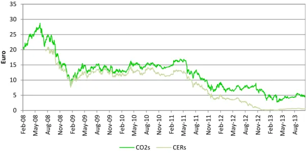
Figure 7 : EU carbon prices, 2008/2013. ... 50

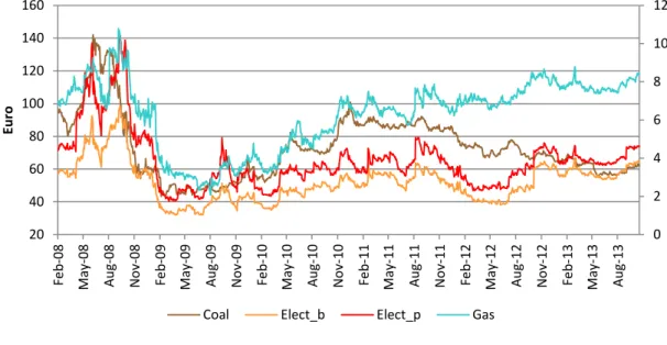
Figure 8 : EU selected energy prices, 2008/2013. ... 52

Figure 9 : EU prices - Granger causality tests ... 55

Figure 10 : Variance decomposition of carbon and electricity prices - EU ... 57

Figure 11 : CO2 price returns accumulated responses to impulses in other variables - EU ... 58

Figure 12 : Impulses in CO2 prices and accumulated responses of selected EU prices ... 60

Figure 13 : Other accumulated impulse-response functions of energy prices - EU ... 62

Figure 14 : Causality cycles between electricity and gas prices - EU ... 63

Figure 15 : Other causality cycles: the role of coal – EU ... 63

Figure 16 : Other causality cycles: the role of gas - EU ... 64

Figure 17 : EU prices - time-series plot and time-series wavelet power spectrum ... 65

Figure 18 : EU prices - wavelet coherence and phase-differences ... 67

Figure 19 : EU prices - partial wavelet coherence and partial phase-differences ... 69

Figure 20: California carbon prices, 2011/2013 ... 80

Figure 21 : California selected energy prices, 2011/2013 ... 82

Figure 22 : California prices - Granger causality tests ... 84

Figure 23 : Variance decomposition of carbon and electricity prices - CA ... 86

Figure 24 : CO2 price returns accumulated responses to impulses in other variables - CA ... 87

Figure 25 : Impulses in CO2 prices and accumulated responses of CA prices. ... 90

Figure 26 : Other accumulated impulse-response functions of energy prices - CA ... 91

Figure 27 : Other causality relations of CO2 - CA ... 91

Figure 28 : CA prices - time-series plot and time-series wavelet power spectrum ... 93

Figure 29 : CA prices - wavelet coherence and phase-differences ... 94

(14)

(15)

INDEX OF TABLES

Table 1 : Power generation in California, per source and geographic origin ... 76

(16)

(17)

ABBREVIATIONS

AAU assigned amount unit

AB32 assembly bill 32

ACV auto covariance

AR auto regression

AR5 assessment report 5

BBL barrel

BTU British thermal unit

CARB California air resources board

CCA California carbon allowance

CDM clean development mechanism

CDS clean dark spread

CER certified emission reduction

CIF Cost, insurance, freight

CO2 carbon dioxide

CO2e CO2 equivalent

COI cone of influence

CSS clean spark spread

CWT continuous wavelet transform

EC European Commission

EEX European energy exchange

EF emission factor

EIA energy information administration

ENSO El Niño southern oscillation

EPA US environmental protection agency

EU ETS European Union emissions trading scheme

EUA European Union allowance

GARCH generalized autoregressive conditional heteroskedasti-city

GDP gross domestic product

GHG greenhouse gas

ICE (The) intercontinental exchange

IPCC intergovernmental panel on climate change

IRF impulse response function

JI joint implementation

LR likelihood ratio

MMBTU million BTU

MWA multivariate wavelet analysis

NA2050 North America 2050

NAS national academies of sciences

NOX mono-nitrogen oxides

OLS ordinary least squares

RAWS remote automated weather stations

RGGI regional greenhouse gas initiative

SO2 sulfur dioxide

STFT short time Fourier transform

SVAR structured VAR

tCO2 tonne of CO2

UNFCCC united nations framework convention on climate change VAR vector autoregression

VMA vector moving average

WCI western climate initiative

Wh Watt hour

(18)

(19)

VARIABLES

EU ETS (prices)

CO2 1 EUA

CER 1 CER

ELE_b baseload electricity price 1 MWh

ELE_p peak electricity price 1 MWh

Coal 1 tonne coal

Gas 1 MMBTU

Econ or FTSE

economy performance index 1 unit

AB32 (prices)

CO2 1 CCA

ELE electricity price 1 MWh

Gasoline 1 gallon

Coal 1 tonne coal

Gas 1 MMBTU

Oil 1 USbbl

Econ economy performance index 1 unit

UNITS

Symbol Factor

G Giga = 109

M Mega = 106

k Kilo = 103

MM Million = 106

-- Trillion = 1012_{(short scale)}

t Tonne = 103_kg = 106_g

g gram

(20)

(21)

1 INTRODUCTION

Global warming is a circumstance of our time coupled to activity of Humankind. Since the

Indus-trial Revolution, the burning of fossil fuels has escalated, increasing the concentration of

green-house gases (GHG) in the planet’s atmosphere (IPCC 2007). The accumulation of those gases creates a greenhouse effect that keeps our planet temperature in an equilibrium. However,

when GHG concentration is above ideal levels, global temperatures rise, causing changes in the

Earth’s climate.

The United Nations Framework Convention on Climate Change, UNFCCC (1992), in its article 1,

n.2, p.3, defines anthropogenic climate change as “a change of climate which is attributed di-rectly or indidi-rectly to human activity that alters the composition of the global atmosphere and

which is, in addition to natural climate variability, observed over comparable time periods”. An-thropogenic climate change has also become known as global warming. To support this

defini-tion, the Intergovernmental Panel on Climate Change (IPCC), the scientific body for the UNFCCC,

gathered research supporting an increase in the average temperature of Earth’s surface by 0.74C since the 19th century. If no action is taken, the IPCC forecasts a rise up to 1.4°C to 5.8°C above

1990 levels, by 2100 (Meehl and al 2007). This unfortunate prediction is recognised by major

National Science Academies (NAS 2005, AAAS 2009, AGU 2013).

In its most recent report (Assessment Report 5 – AR5), the IPCC identifies a GHG emissions budget1_{of 840Gt. This carbon budget would allow the world to have a 50% chance of staying}

below 2ºC of warming by 2100, above 1861-1880 levels (IPCC 2013). Current emission rates are

at 10GtC per year and about 531GtC has already been used (IPCC 2013). So, without additional

action, in 30 years the budget will have been used. With this knowledge, effects of global

warm-ing, such as melting glaciers and more frequent extreme weather events, that can already be

felt in some parts of the globe, are estimated to worsen in the coming decades (EC 2013a). As

an example, under a high emissions scenario, by 2050 the Arctic Ocean is expected to have no

ice during the summer (IPCC 2013). In fact, the IPCC states that about 20-30% of plant and animal

species is likely at higher risk of extinction if the global average temperature goes up by more

than 1.5 to 2.5°C (IPCC 2007). In short, the IPCC points out consequences such as «agricultural

yields expected to drop […]; diseases […] could spread to new areas in the world; millions of

(22)

people expected to be exposed to increase water stress; more intense weather-related

disas-ters; and extinctions» UNFCCC (2007), p.1. Sectors such as agriculture, energy and tourism, very

dependent on the level of temperature, precipitation and sea level, will, thus, be particularly

affected by global warming (EC 2013a).

It is reasonable to say that climate change will globally have harmful effects on societies and the

economic and natural systems in which they live.

In this context, the UNFCCC, created in 1992, has the goal of achieving the «stabilization of

greenhouse gas concentrations in the atmosphere at a level that would prevent dangerous

an-thropogenic interference with the climate system. Such a level should be achieved within a

time-frame sufficient to allow ecosystems to adapt naturally to climate change, to ensure that food

production is not threatened and to enable economic development to proceed in a sustainable

manner» (UNFCCC 1992), article 2, p.4. 195 countries ratified this overall global objective,

prom-ising to engage in mitigation actions, that is, actions that reduce net carbon emissions and limit

long-term climate change (IPCC 2007). An important concept in climate change and carbon

eco-nomics is “mitigation”, the act of decreasing future global warming.

With the mitigation purpose in mind, Governments have a very important role of engaging

pol-luting companies and the society in reducing their emissions. There are essentially two policy

instruments that help attain the desired goal: either command-and-control imposed regulations,

or economic incentive instruments.

The first option, to enforce emission limits, is rather inflexible and does not provide an incentive

for emitters to engage in further reductions beyond the imposed limit. Also, imposed regulations

are known to be less efficient and less cost-effective than other options, for they rely on a

pre-cise definition of the conditions and quantities of emissions, which are uncertain to a certain

point (Tietenberg and Lewis 2009).

Alternatively, as economic incentive instruments to control emissions we find taxes and

cap-and-trade, although cap-and-trade includes a command and control feature regarding the

pol-lution limit that must be defined. Both trading and taxes recognize a market failure stemming

from a negative externality. Atmospheric pollution constitutes a negative externality because

polluters do not compensate society for the damage they cause. “Climate change is the greatest market failure the world has ever seen” (Stern 2006). To address these climate externality costs, cap-and-trade bounds a “set amount” of emissions, while taxes work indirectly.

Emission taxes are defined in the form of a Pigouvian tax where the negative externality is

(23)

theoretical economic system conditions, such as perfect information, rational agents and no

transaction costs, both tools, taxes and cap-and-trade, should reach a set amount of emission.

They both put a price on carbon, thus consequently correcting the market failure. However,

while cap-and-trade provide certainty on emission quantities, taxes, on the other hand, are only

‘cost’ certain (Helm 2005).

The idea of a cap-and-trade, or an emission market mechanism, was initially born in a study by

Coase (1960) regarding property rights. Under certain conditions, by clearly defining property

rights, and making them exchangeable, the market would give a value to those rights and

allo-cate them to “their best use”, as Tietenberg (2010) poses. After Coase, Crocker (1966) applies the concept to air pollution and Dales (1968) to water. Baumol and Oates (1971), p.42,

corrob-orate the idea stating that “for any given vector of final outputs such prices can achieve a

spec-ified reduction in pollution levels at minimum cost to the economy”. Greenhouse gases pollution are an example of Baumol and Oates idea, which only applies when all emissions have the same

impact on the environment. In this case, GHGs have the same impact regardless of the location

from where they are emitted.

In emission control policy, preference has been shown for emissions trading over the imposition

of taxes. The main reason for market-preference is the acknowledgment that generated

reve-nues are automatically distributed to companies in the market, rather than collected by the

Government (Metz and al 2001), although it should depend on the final use of tax revenues, and

markets transaction costs. In addition, the argument that the knowledge of abatement costs is

not complete reinforces the uncertainty in the amounts of emissions reductions that the tax will

achieve (Smith 2008), referred above as the “quantity certainty” of results.

On operational issues, emissions trading requires, in the first place, the definition of an overall

limit on emissions, and the issuance of the equivalent number of permits. Market participants

will need to hold the number of permits that correspond to their actual emissions. The trading

of permits is allowed, thus allocating reductions to actions with lower marginal costs, regardless

of the initial allocation. In this sense, by achieving optimal abatement level at a minimum cost,

the cost-effectiveness of the system is ensured (Tietenberg 2003).

First microeconomic computer simulations of a cap-and-trade system for cities emissions were

designed by Burton and Sanjour, between 1967 and 1970 (Burton and Sanjour 1970, Burton et

al. 1973), for the National Air Pollution Control Administration (now called the US Environmental

(24)

on emission markets operation (Burton and Sanjour 1970, Burton et al. 1973). In 1985

Tieten-berg published a review of an emissions exchange system between plants in a same company,

which EPA allowed. He shows that the system provided the right incentives for innovation and

investment in emission control, presenting proof of principle that previously simulated

emis-sions trading is a new policy instrument (Tietenberg 1985). At that time countries were having a

large problem with “acid rain”, mainly caused by sulphur dioxide and nitrogen oxides, from fossil

fuel-burning power plants, especially coal power plants. To deal with this issue, the first “ cap-and-trade” system was conceived by C. Boyden Gray, under the Clean Air Act, as part of the US Acid Rain Program (Voß 2007, Calel 2011). Trading of permits between power plants started in

1995. Assessment studies show that the original limit or ‘cap’ goal was reached in 2007, way

before the 2010 deadline, and with only one fourth of the initially expected costs (EPA 2007,

Napolitano et al. 2007).

Other emissions cap-and-trade examples existed, although small when comparing to the Acid

Rain Program in terms of participants involved and emissions’ reductions (Ellerman and Harrison Jr 2003): the “RECLAIM” program, capping NOX (mono-nitrogen oxides) and SO2 (sulfur dioxide) stationary emissions in the Los Angeles Basin, since 1994, and the “Northeast NOX Budget

Trad-ing”, trading NOX, in the Northeastern US since 1999.

On GHG, the European Union Emission Trading Scheme (EU ETS) was the first market to be

im-plemented, in 2005. It is still by far the largest (EC 2013b), including most energy intensive

sec-tors of the economy, currently with obligations up to 2020. In the USA, the Regional Greenhouse

Gas Initiative (RGGI) started in 2009, and is a trading system for power generators. Also in the

USA, the state of California has a cap-and-trade program for GHG emissions that started

opera-tions in early 2012, with mandatory compliance since January 1, 2013. Far from there, in China,

four towns and a province are under regional emission markets covering power generators.

Guangdong, the province, is expected to have the second-largest carbon market in the world,

after the EU ETS, pairwise to the California program. Other markets for GHG exist, in Australia,

New Zealand, the City of Tokyo, Kazakhstan, Switzerland, and Quebec. Most of these markets

started in 2012-2013. Another three emission trading schemes are scheduled for launching, and

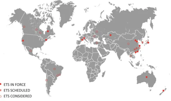
15 are considered for implementation, as we may see in Figure 1.

In summary, in the last 20 years we find good results from the initial studies and simulations, we

have an “Acid Rain” emissions market that rendered high positive outcomes, and international

policy preference for cap-and-trade rather than direct regulation or taxes. Also, the EU ETS is in

its third phase, and other 12 markets are in place. We may say, against this background, that

(25)

must be liquid, transparent and efficient, to assure their primary goal of capping GHG emissions

at the least cost for society.

Figure 1 : Emission trading schemes around the World

(data source: icapcarbonaction.com)

Under a cap-and-trade system, emission prices are of the utmost importance. They reflect the

‘price of pollution’, or the marginal cost of abatement, providing actors with ongoing incentives

for technological changes that reduces emissions. Carbon prices present the equilibrium

be-tween demand and supply of emission permits, and consequently are the mirror of abatement

decisions. Tietenberg (2010), p.3, recalls that in this scheme, prices are instantly determined,

avoiding a “long iterative procedure […] through trial and error […] found in tax and standards

system”. The carbon price also conveys useful information to climate policy, which can thus con-sciously decide on the overall emissions goal (Aatola et al. 2013b). So, expectedly, a large part

of studies on carbon markets look at price variations, determinations and effects, as will be

re-ferred in the following chapters.

Looking in particular to the EU ETS, the reference carbon market because of its age and size, one

can observe a very evident price decline since the beginning of its operations, in 2005. Since

2008, prices dropped from a maximum of € 28.73 to 2.7€ /tCO2e, averaging 4.4€/tCO2e in 2013

(Bluenext and SendeCO2 data). Also, studies have demonstrated the existence of arbitrage

(26)

that the exchange of allowances at less than 8 € / tonne is too low to encourage investment in

energy efficiency or 'low carbon' energy, adding that the system has to be improved to raise

prices and achieve increased stability. Finally, Löfgren et al. (2013) and Lundgren et al. (2013)

show the lack of a significant effect on companies decisions to invest in the development of

mitigation technologies based on low EU ETS carbon prices.

Nevertheless, the EU ETS continues to be the European Union primary climate change policy

tool, presenting small, but real net emissions reductions additional to other EU sustainability

measures (Branger et al. 2013). And so, regardless of price forecasts and criticisms, it is expected

that the review of the European carbon market, which began in 2013, will establish stronger

links between commitments to reduce emissions of individual European countries (Egenhofer

and Alessi 2013), and will achieve some control over the price of carbon (Branger et al. 2013).

More recently, the European Commission presented the “2030 climate and energy goals for a

competitive, secure and low-carbon EU economy” (EC 2014) 2_{. The EC proposal has six key} en-ergy-climate elements, including the reduction in GHG emissions by 40% below the 1990 level

and the reform of the EU ETS. Regarding changes in the EU ETS, the EC (2014), p.1 “proposes to

establish a market stability reserve […] that would both address the surplus of emission

allow-ances that has built up in recent years and improve the system's resilience to major shocks by

automatically adjusting the supply of allowances to be auctioned”. Also, estimates by the leading

source of information on carbon trading indicate prices between 21€/tCO2e and €96/tCO2e for 2030 depending on the rate of economic growth (Schjølset, PointCarbon), which translates the

high uncertainty about the dynamics of the carbon price and its feedback effects on other energy

variables. In view of the importance that energy prices have on energy and climate issues, and,

in consequence, on the EU ETS, the EC attaches to the 2014 proposal a “Report on energy prices

and cost”.

Of course, GHG emissions and energy use are tangibly related, so, this relation should reveal

itself in the corresponding exchange markets. Emission market fundamentals previously

pre-sented tell us that the carbon price should reflect the negative pollution externality. Thus,

en-ergy markets should act accordingly in the presence of a pollution production cost, penalizing

the use of more emitting fuels. Also, changes in more more or less polluting energy prices should

also be reflected in the carbon price. Many authors have discussed causality between carbon

and electricity, natural gas and coal prices, and, longer term effects of institutional and policy

(27)

decisions (Asafu-Adjaye 2000, Springer and Varilek 2004, Mansanet-Bataller et al. 2007,

Milunovich 2007, Alberola et al. 2008, Benz and Truck 2009, Fezzi and Bunn 2009,

Mansanet-Bataller and Soriano 2009, Hintermann 2010, Keppler and Mansanet-Mansanet-Bataller 2010, Chevallier

2011d, Feng et al. 2011, Conrad et al. 2012, Gorenflo 2012, Sijm et al. 2012, Aatola et al. 2013a,

b, Byun and Cho 2013, García-Martos et al. 2013, Kopp and Mignone 2013, Liu and Chen 2013,

Lutz et al. 2013).

The studies on relations between energy and carbon prices, as typical finance markets research,

follow econometric methodologies. These approaches allow to quantify relations and, more

than that, test hypotheses with scientific rigor3_{. Within the vast econometrics models that exist,}

Granger causality tests (Granger 1969) have been used for interconnection analysis between

CO2 prices and other variables (Keppler and Mansanet-Bataller 2010, Creti et al. 2012). Although

it can be repeated on both ways, Granger tests only consider a one-way influence of variables

in CO2 at each moment, while everything else remains constant. In short, the Granger causality

test studies the hypothesis of one time series being statistically significant in predicting another.

We may say that the series ‘A’ Granger-causes ‘B’. However, this approach has limitations mostly because the test is designed to handle pairs of variables, problems arising when there is a

pos-sibility of the existence of a ‘C’ series that can move both A and B. And, in fact, the reality in carbon-energy analysis is that a feedback effect of price variations is expected (Keppler and

Mansanet-Bataller 2010).

The mathematical solution to overcome the pairwise endogeneity issue is to use a vector of

several endogenous variables as dependent and their lagged values as independent variables.

In econometrics this is called a vector autoregression model (VAR) which is usually applied to

analyse and display interdependencies between different interrelated time series. The main

fea-ture of this model is to allow the study of impulse-response functions (IRF) that consider the

influence of all time series at the same time. In this function, an impulse, or innovation, is given

to one variable, and responses are analysed in other variables.

There are recent studies related to carbon markets that use VAR models, but they apply this

methodology to stock prices of clean energy firms, oil and carbon markets (Kumar et al. 2012),

3_{“Reasoning on economic facts means, and always meant, within a}_{very important sector, quantitative}

reasoning. And there is no logical breach between quantitative reasoning of an elementary character, and

(28)

to the role of macroeconomic indicators (Chevallier 2011c, Chevallier 2011d) or look at the

im-pacts of changes in electricity prices (Aatola et al. 2013b). However, these studies are not

di-rectly related to carbon versus energy prices. There is also a study by Fezzi and Bunn (2009) that

studies impulse-responses although exclusively between gas, carbon and electricity, in the UK

for the first phase of the EU ETS. Finally, Gorenflo (2012) also relies on a VAR model to study the

lead–lag relationship between spot and futures prices of CO2 emission allowances. Other au-thors look into volatility issues, mostly through GARCH models (Benz and Truck 2009, Chevallier

2011b, Arouri et al. 2012, Conrad et al. 2012, Rittler 2012, Byun and Cho 2013, Liu and Chen

2013, Koch 2014, Reboredo 2014). A more detailed literature analysis on carbon prices is

pre-sented in the introduction of the analysis chapter, section 3.1.

In this study, we propose to go deeply on the analysis of carbon price dynamics. Looking at

re-cent data from two large carbon trading schemes, we aim to analyse the interrelationship of CO2

prices with the most relevant energy, economy and substitute goods influencing those markets.

Scientific contributions, research questions and proposed hypotheses

Therefore, as the first scientific contribution of this work, we specify a dynamic vector auto-regression (VAR) model to estimate response functions of CO2 prices to impulses in other

var-iables, and vice versa. These impulse-response functions (IRF) allow us to observe the impact of CO2 in other variables, in terms of duration, direction and magnitude.

In complement to the previous model from which we obtain short-term responses, we also study longer cycles through wavelet analysis. This is the second scientific contribution of this work. This analysis is done simultaneously in the time and frequency domains, in complement to the time-domain method that is a VAR. This allow us to see how carbon and energy prices

behave at different frequencies and how this behaviour changes over time. Since wavelet

anal-ysis provides convenient tools to distinguish relations at particular frequencies and particular

time horizons, our empirical approach has the potential to identify relations getting stronger

and then disappearing over specific time intervals and frequencies. With this method, we will

(29)

relations, at different frequencies for the time period in focus. This is useful longer term

infor-mation that the VAR impulse-response function does not provide. To our knowledge we are the

first to apply multivariate wavelet analysis, proposed by Aguiar-Conraria and Soares (2014). We propose to develop such a study on two carbon markets: the largest and oldest carbon

mar-ket – the European, and the newest and promising Californian carbon market.

These two approaches will increase the evidence on this subject by providing us with suggestions

on how much cost variation from emissions should be expected and for how long. It will deliver

a causality analysis of endogenous variables expected to influence and to be influenced by the

carbon price, and impact duration and direction of changes in those variables.

Our two main research questions include the identification of carbon price drivers, and effects:

What drives carbon price variations? What variations do carbon prices drive?

Following referred previous studies and carbon market fundamentals we hypothesize a possible

influence of the economy, of both final and primary energies, and of carbon permits substitutes

(offset credits) in the carbon price. In the reverse view, we consider that carbon prices mainly

influence final energy prices, although not discarding the possibility of also influencing gas or

coal prices. We propose that the influence of energy prices in CO2 prices happens in the very

short-term. We also propose that the potential impact of carbon prices in final energy prices

occurs in a one year cycle, or more, if considering primary energies prices. Our methods do not

impose theoretical assumptions4_.

If we look at different variables, and consider the sectors included in the emission markets, the

above presented hypotheses can be divided into several research sub-questions.

(30)

On carbon price drivers:

1. Do final energy prices impact carbon price?

We hypothesize positive immediate reactions from impacts of electricity and gasoline.

2. Do primary energy prices impact carbon price?

We expect so, in a very immediate term, and expect a positive relation originating from

gas prices, and negative from oil and coal. Regarding the existence of substitutes for

carbon licences, we do not expect a significant effect on the carbon price.

3. Finally, on the macroeconomic perspective, does the level of economic activity trans-lates into the carbon market?

Yes, we hypothesize a positive, fast, reaction.

On carbon price effects:

1. Does carbon price influences final energy prices, including electricity and gasoline? We hypothesize a positive relation.

2. Does carbon prices influence primary energy prices, including natural gas, coal and oil? We hypothesize a negative relation towards coal prices and positive relation regarding

gas and oil.

3. Does the permit price impact the offset price (CER) in the EU ETS?

In the EU ETS, CERs, or credits from emission reduction projects (offsets) may be used

in a limited way as alternative compliance tool to the European Union allowance. We

(31)

In the context of the economic crisis affecting Europe since 2007, and for the proper start-up of

the Californian market, it is particularly important to respond to the previous questions,

identi-fying what drives carbon prices and how they do reflect market fundamentals. A detailed study

of this matter carries valuable results to policy and production decisions. Only with a more

com-prehensive knowledge on carbon price origins and effects, a proper evaluation of the market

policy effectiveness will be possible and market actors will be able to implement necessary

measures to obtain the desired outcomes of reducing emissions, moving towards efficiency.

This document follows a very simple structure: in chapter two we describe the econometric

the-ory used in the VAR models and Wavelet analysis. The wavelet section has more detail because

we use instruments not yet used (e.g. multivariate wavelet analysis). Chapter three

character-izes the European and the Californian markets, data, and results. In chapter four we discuss the

methodology and comment on policy implications from both models and markets, and finally

chapter five concludes and proposes directions for further research.

(32)

(33)

2 METHODOLOGY

In this chapter we present the methodological and theoretical framework, essentially from a

mathematical standpoint.

First we present the construction of the vector auto-regressive model and finally the deduction

of the partial multivariate analysis tools is outlined.

The application of this method to our analysis is justified in the introduction to Chapter 3. At

that point, after this theoretical background, the interest of this innovative approach to the

anal-ysis of carbon prices will become clear.

The data and MatLab scripts necessary to replicate all our wavelet analysis results are available

for download at http://sites.google.com/site/aguiarconraria/joanasoares-wavelets. In the same

website, the reader can find and freely download a wavelet MatLab toolbox, The ASToolbox,

written by Maria Joana Soares and Luís Aguiar-Conraria. Regarding the VAR analysis, the Eviews

data files necessary to replicate all our results are available for download at

http://www.rita-sousa.com.

2.1 The Vector Autoregression Model (VAR)

2.1.1 Background on VAR models

In time series, a vector autoregression (VAR) model is a natural expansion of the one-variable

autoregression model (AR). In an AR model the variable depends on its past values, whereas a

VAR model allows for a vector of several evolving variables. VAR models became famous in

Chris-topher A. Sims’ paper “Macroeconomics and Reality” (Sims 1980).They are linear models with n variables, thus n equations, where each variable is explained by its own lagged values and

pre-sent and past values of all other variables. In this section we contextualize the use of VAR models

and in the next present the VAR theory.

There is a substantial number of relevant references on VAR time series models (Tiao and Tsay

1989, Amisano and Giannini 1997, Stock and Watson 2001, Enders 2008, Tsay 2010, Peña et al.

2011).The following demonstrations are necessarily brief, because the methodology is of

(34)

The VAR framework delivers an efficient and flexible way to observe the dynamics in multiple

time series. As Stock and Watson (2001) p.1 pose, the VAR work by Sims, “held out the promise

of providing a coherent and credible approach to data description, forecasting, structural

infer-ence, and policy analysis”. It has been widely used to analyse economic and financial time series and for forecasting. However, the problem of defining causality with several variables is still

challenging, and institutional knowledge and economic theory must always be considered in the

analysis of the model results. This is especially important in structural inference and policy

anal-ysis, because it is necessary to impose assumptions regarding the causal structure.

A central outcome of VAR models is that it allows to estimate the dynamic response of a variable

to innovations in other variables through a set of impulse-response functions (IRF), after

appro-priate restrictions identification.

Causality issues are usually analysed following a Granger-causality test (Granger 1969). A

varia-ble x is said to Granger-cause a variable y if, given the past values of y, past values of x are useful

in forecasting y. VAR models can also be used for testing Granger-causality. Granger causality

relies on correlation between the current value of one variable and the past values of other, so,

if we test for joint the significance of the lagged independent variables, we are testing for

Granger causality. However, it is possible that we find Granger causality in both directions,

al-loying for feedback mechanisms. It is also possible that both variables are driven by a third

var-iable. In this situation it would not be advisable to use a Granger test, because it is designed to

analyse relation between two variables. It may produce distorted results when considering three

or more variables (Stern 2011). In alternative, the Wald test, or block exogeneity test, checks for

variables exogeneity, considering more than two variables, thus, may be applied to VAR models

with n variables. The null hypothesis in the Wald test is that a set of parameters coefficients is

equal to a specific value, in our case, zero. If we do not reject H0, then it suggests that the

vari-ables are possibly exogenous.

In short, the Wald test checks for Granger causality in a VAR model: for each equation and each

endogenous variable that is not the dependent variable in that equation, we compute Wald tests

that the coefficients on all the lags of an endogenous variable are jointly zero, and, that each of

the other endogenous variables does not Granger-cause the dependent variable in that

(35)

Specification issues: variables and lags

To correctly specify a VAR model we need not only to decide on which variables to include, but

also on the on the number of lags. On this regard, it is possible to rely on information criteria, or

formal testing. The Akaike (AIC) and Schwarz-Bayesian (SIC) information criteria are the most

common methods used. However, information criteria are not tests, so they mainly indicate the

goodness of fit of alternative lag number. The alternative is to use formal testing with the

Like-lihood Ratio (LR)5_{, which we used in the models presented in sections 3.2.3 and 3.3.3 (VAR}

anal-ysis of EU and CA, respectively).

In what follows we present two VARs representations, which will be one of the workhorses of

our empirical analyses: the structural (SVAR) and the reduced form (VAR). In the SVAR we follow

econometric theory by Sims (1980) to define the causality relation between variables in the

con-temporaneous period. The main feature is that Sims uses the Cholesky decomposition of the

VAR variance-covariance error matrix. Others decomposition methods exist, such as Blanchard

and Quah (1989), this one more adequate to long-run restrictions. The reduced form VAR,

de-duced from the SVAR, considers a serially uncorrelated error term, where each equation is

esti-mated by ordinary least squares, and allows the estimation of the impulse-response functions.

2.1.2 Theory of a VAR model

2.1.2.1 VAR Analysis

As previously introduced, a vector auto-regressive model presents the simultaneous evolution

of a set of variables. These variables are endogenous, which is saying that they evolve as a

func-tion of all their previous values. They may be represented in a vector_𝑌_𝑡, where t is the period

observed in each of the n variables:

𝑌𝑡 = [𝑦1𝑡 𝑦2𝑡 … 𝑦𝑛𝑡]𝑇 (1)

5_{The LR test statistic is:}_{𝐿𝑅 = (𝑇 − 𝑚)(ln|Σ}

𝑟| − ln|Σ𝑢|) ~ 𝜒2(𝑞) with T = number of observations (after

(36)

In this work our time series will include carbon prices, electricity prices, and natural gas prices,

among others, as presented next in section 2.2.1.

For simplicity purposes, following Enders (2008), we first show the determination of a two

vari-ables and one lag, or, VAR(1) model. Then, we generalize to a VAR(p) of n variables.

Consider the following model with two variables that depend simultaneously on each other and

also on their lagged value:

𝑦1𝑡 = 𝑐10− 𝑏12. 𝑦2𝑡+ 𝑐11. 𝑦1,𝑡−1+ 𝑐12. 𝑦2,𝑡−1+ 𝜀𝑦1𝑡

𝑦2𝑡 = 𝑐20− 𝑏21. 𝑦2𝑡 + 𝑐21. 𝑦1,𝑡−1+ 𝑐22. 𝑦2,𝑡−1+ 𝜀𝑦2𝑡

Where _𝜀_𝑦_𝑖_𝑡 is an i.i.d. error term with mean zero, with _{𝑐𝑜𝑣(𝜀}_𝑦₁_{, 𝜀}_𝑦₂_{) = 0}. In matrix form:

[ 1_𝑏 𝑏12

21 1 ] [

𝑦1𝑡

𝑦2𝑡] = [

𝑐10

𝑐20] + [

𝑐11 𝑐12

𝑐21 𝑐22] [

𝑦1,𝑡−1

𝑦2,𝑡−1] + [

𝜀𝑦1𝑡 𝜀𝑦2𝑡]

Which can be written more compactly written as:

𝐵𝑌𝑡 = Γ0+ Γ1𝑌𝑡−1+ 𝜀𝑡 (2)

Equation (2) is called the structural VAR (SVAR).

Matrix _𝐵 reports the contemporaneous relations between variables, or, in other words, the

ef-fect that a variable in one moment has in the other in that same moment. So the model allows

for feedback effect because variables at time ‘t’ may affect each other.

Unfortunately, equation (2) cannot be estimated directly by ordinary least squares (OLS), as they

would render inconsistent estimates.

(37)

𝐵−1_𝐵𝑌

𝑡 = 𝐵−1Γ0+ 𝐵−1Γ1𝑌𝑡−1+ 𝐵−1𝜀𝑡

Which may be simplified to an unstructuredVARusually called VAR, in standard form:

𝑌𝑡 = A0+ A1𝑌𝑡−1+ 𝑒𝑡 (3)

The new error terms _𝑒_𝑡 are composites of the _𝜀_𝑡 errors, or innovations, from the SVAR.

Equation (3) delivers the VAR in its reduced form and can be estimated by OLS. Note that the_𝑒_𝑡’s have zero mean and constant in time independent variances, but their covariances are not zero,

meaning that although they are serially uncorrelated, they are correlated across equations. I.e.,

the shocks in the model are correlated.

For clarity, we may represent the result of the 2 variables VAR(1) in the matrix form:

[𝑦_𝑦1𝑡

2𝑡] = [

𝑎10

𝑎20] + [

𝑎11 𝑎12

𝑎21 𝑎22] [

𝑦1,𝑡−1

𝑦2,𝑡−1] + [

𝑒1𝑡

𝑒2𝑡] (4)

Generalizing the model to n variables and p lags, a vector auto-regressive model explains the

value of all variables included in vector_𝑌_𝑡 in current period t with their own values in previous

periods. It is an auto-regression of the vector of variables in previously determined p lags, also

called a pth-order VAR. Following equation (2), the SVAR(p) may be written as:

𝐵𝑌𝑡 = Γ0+ Γ1𝑌𝑡−1+ Γ2𝑌𝑡−2+ ⋯ + Γ𝑝𝑌𝑡−𝑝+ 𝜀𝑡 , ∀(𝑡, 𝑝) ∈ ℕ (5)

And then, again, pre-multiplying by _𝐵−1, we obtain the VAR model:

𝑌𝑡 = A0+ 𝐴1𝑌𝑡−1+ 𝐴2𝑌𝑡−2+ ⋯ + 𝐴𝑝𝑌𝑡−𝑝+ 𝑒𝑡 , ∀(𝑡, 𝑝) ∈ ℕ (6)

(38)

Next, we represent the model in lag polynomials to make it more practical6_{. We may then}

rep-resent equation (5), the SVAR(p), as:

𝐵𝑌𝑡 = Γ0+ Γ1(𝐿)𝑌𝑡−1+ 𝜀𝑡 (7)

And finally obtain the VAR(p):

𝑌𝑡 = A0+ A1(𝐿)𝑌𝑡−1+ 𝑒𝑡 (8)

Again, equation (8) delivers the VAR in its reduced form and can be estimated by OLS. Once

more, as in equation (3), _𝑒_𝑡’s have zero mean and constant time independent variances, but their covariances are not zero, meaning that although they are serially uncorrelated, they are

correlated across equations. I.e., the shocks in the model are correlated.

This can easily be illustrated in a VAR(1), 2 variables, example. Recalling the matrix B as

repre-sentative of the contemporaneous effects, and from equation (3) that:

𝑒𝑡 = 𝐵−1𝜀𝑡 (9)

From linear algebra analytical inverse matrix determination, we have:

𝐵−1₌ 1

|𝐵|(𝐵∗)𝑇 = 1

1 − 𝑏21𝑏12[ 1

−𝑏12

−𝑏21 1 ]

With the adjugate matrix = (𝐵∗)𝑇, or, the transposed cofactor matrix.

Rewriting (9) in matrices:

6_{Lag operator, or backshift operator L:}_𝐿𝑌

𝑡= 𝑌𝑡−1 or 𝐿𝑌𝑡+1= 𝑌𝑡, then 𝐿−1𝐿𝑌𝑡= 𝐿−1𝑌𝑡−1⟺ 𝑌𝑡=

𝐿−1_𝑌

(39)

[𝑒_𝑒2𝑡

1𝑡] =

1

1 − 𝑏21𝑏12[ 1

−𝑏12

−𝑏21 1 ] [

𝜀𝑦1𝑡 𝜀𝑦2𝑡]

With the solutions:

𝑒1𝑡 =𝜀𝑦_{1 − 𝑏}1𝑡− 𝑏12𝜀𝑦2𝑡

21𝑏12 𝑎𝑛𝑑 𝑒2𝑡 =

𝜀𝑦2𝑡− 𝑏21𝜀𝑦1𝑡 1 − 𝑏21𝑏12

Because _𝜀_𝑦₁_𝑡 and _𝜀_𝑦₂_𝑡 are white noise, a stationary time series or a stationary random process

with zero autocorrelation, then _𝑒_1𝑡 and _𝑒_2𝑡 have the following moments:

𝐸(𝑒𝑖𝑡) = 0

𝑉𝑎𝑟(𝑒1𝑡) = 𝐸(𝑒𝑖𝑡2) =𝐸(𝜀𝑦1𝑡 2 _{+ 𝑏}

122 𝜀𝑦22𝑡) (1 − 𝑏21𝑏12)2 =

𝜎𝑦21+ 𝑏122 𝜎𝑦22 (1 − 𝑏21𝑏12)2

(10)

We obtain similar results to equation (10) for _{𝑉𝑎𝑟(𝑒}_2𝑡₎.

On covariance:

𝐶𝑜𝑣𝑎𝑟(𝑒1𝑡, 𝑒2𝑡) = 𝐸(𝑒1𝑡. 𝑒2𝑡) =

=𝐸[(𝜀𝑦1𝑡− 𝑏12𝜀𝑦2𝑡)(𝜀𝑦2𝑡− 𝑏21𝜀𝑦1𝑡)] (1 − 𝑏21𝑏12)2 =

−𝑏21𝜎𝑦21− 𝑏12𝜎𝑦22 (1 − 𝑏21𝑏12)2 ≠ 0

(11)

So, the shocks in the SVAR are correlated. The contemporaneous effects reflected in matrix B by

(40)

2.1.2.2 Cholesky decomposition

Given the contemporaneous effects presented in B, it is not possible to use OLS to estimate the

SVAR. To overcome this issue, one has to estimate the VAR in the reduced form. Unfortunately,

from that estimation it is not possible to recover the structural parameters of interest. To do so,

one needs to add extra restrictions.

We follow the methodology proposed by Sims (1980) and rely on the Cholesky decomposition

to impose short run identification restrictions. The idea is to impose restrictions in the error

covariance matrix of equation (8) in order to recover matrix _𝐵 of equation (7). These restrictions

impose contemporaneous effects of zero in a predetermined direction. By a convenient ordering

the variables, we basically impose that the covariance matrix is lower triangular where the first

equation does not consider any other innovation rather than its own, the second equation

con-siders the second and the first coming from the addition of the first equation and so on, until

the last equation that considers them all. In the VAR(1) example, with a Cholesky

decomposi-tion7_,_B_{matrix becomes:}

𝐵 = [ 1_𝑏 0

21 1] 𝑡ℎ𝑢𝑠 𝐵

−1_{= [ 1} 0

−𝑏21 1]

hence VAR(1):

[𝑦_𝑦1𝑡_2𝑡] =

= [_𝑐₂₀_{− 𝑏}𝑐10₂₁_𝑐₁₀] + [_𝑐 𝑐11 𝑐12

21− 𝑏21𝑐11 𝑐22− 𝑏21𝑐12] [

𝑦1,𝑡−1

𝑦2,𝑡−1] + [

𝜀𝑦1𝑡 𝜀𝑦2𝑡− 𝑏12𝜀𝑦1𝑡]

(12)

Comparing equations (4) and (12) we obtain the coefficients of the VAR:

7_{Considering a symmetric positive-definite matrix A, a Cholesky decomposition factorizes A into the}

(41)

𝑎10 = 𝑐10, 𝑎11 = 𝑐11, 𝑎12= 𝑐12, 𝑒1𝑡= 𝜀𝑦1𝑡

𝑎20= 𝑐20− 𝑏21𝑐10, 𝑎21= 𝑐21− 𝑏21𝑐11, 𝑎22= 𝑐22− 𝑏21𝑐12, 𝑒2𝑡 = 𝜀𝑦2𝑡− 𝑏12𝜀𝑦1𝑡

It is visible in the previous deduction that results will depend on the chosen variable order of

impact in the contemporaneous period. In the example, if instead we had considered b21=0, the

results would have been different. Changing the order does not render significative changes in

the results when the correlation between errors is small (Enders 2008).

2.1.2.3 Impact multipliers and Impulse Response Functions (IRF)

An impulse, or an impelling force or motion, is what is assumed to trigger the dynamic response

of the model. The goal is the analysis of the response, the propagation mechanism, of the

vari-ables in the following time periods. The IRF shows the effect of a particular innovation to variable 𝑖 (_𝜀_𝑖,𝑡) on the contemporaneous and future values of all variables.

The process to define these functions starts with the estimated ‘composite’ 𝑒𝑡 residuals (linear

combinations of uncorrelated innovations) and from them rebuilds the original innovations _𝜀_𝑡.

The process involves representing the VAR model as a Vector Moving Average (VMA) where

endogenous variables are defined by _𝑒_𝑡 shocks (Sims 1980). The VMA allows tracking the shocks

effects. To see this, note that equation (8) may be rewritten as:

𝐴(𝐿)𝑌𝑡= 𝑒𝑡 (13)

Where, for simplicity, we dropped the constants and _{𝐴(𝐿) = (𝐼 − 𝐴}₁_(𝐿)).

Then, considering the VAR model is invertible, it is possible to write equation (13) as a Vector

Moving Average of infinite order _{𝑉𝑀𝐴(∞)}:

𝑌𝑡 = 𝐴−1(𝐿)𝑒𝑡 = 𝐴−1(𝐿)𝐵−1𝜀𝑡 = Φ(L)𝜀𝑡 (14)

It should be clear from equation (14), that with a VMA representation, and keeping in mind that

𝑒𝑡 = 𝐵−1𝜀𝑡, it is possible to estimate the impulse response function. Given a unit change in

(42)

𝜕𝑦𝑖,𝑡+𝑠

𝜕𝜀𝑗,𝑡 = Φ𝑖,𝑗(𝑠) (15)

Equation (15) shows the impact effect of a one unit change in _𝜀_𝑗, a structural innovation, on _𝑦_𝑖,

in s lags. Impulse response functions (IRF) are the representation of the effects of structural

innovations on current and future values of considered variables _Φ_𝑖,𝑗_{(0), Φ}_𝑖,𝑗_{(1), Φ}_𝑖,𝑗_{(2), …}

They are the time path of dependent variables. For each n variables model we have n2_IRFs.

When the system of equations is stationary, the impact also becomes stable after some periods.

(43)

2.2 Multivariate Wavelets Analysis

2.2.1 Background on wavelet analysis

In the previous section, we considered the simultaneous analysis of multiple variables

dynami-cally explained by all of them in past periods. This is a very useful approach if we consider a fixed

frequency of data, in this case, daily prices. However, in a time series there may exist periodic

signals which vary in amplitude and frequency over time, and therefore provide additional

in-formation beyond that observed at a fixed frequency. This additional inin-formation may or may

not be captured depending on the methodology used, but one cannot deny the possibility of

existence of different cycles in the same time series.

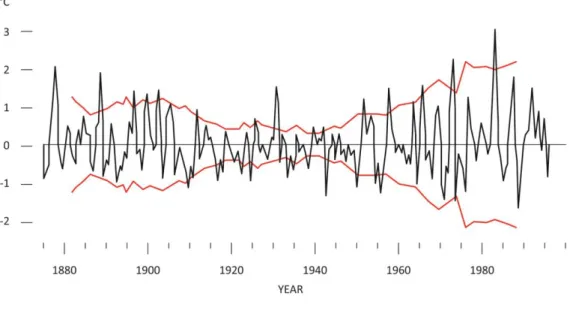
Torrence and Compo (1998) present a very evident example of overlapping temporal

infor-mation at different frequencies: the analysis of sea surface temperature in the equatorial Pacific

Ocean. The most visible temperature variability, originating from the "El Niño - Southern

Oscil-lation" (ENSO), has irregular cycles of 2 to 7 years. But this variation overlaps other longer

fluc-tuations of decades, which modulate the amplitude and occurrence of the phenomena of El

Niño, as shown in Figure 2:

Figure 2 : Sea surface temperatures averaged over the NINO3 area in the eastern Pacific.

Data source: (Torrence and Compo 1998). Black represents the averaged sea surface temperatures of the area

5°S-5°N, 90°W-150°W. Red shows the running 15-year variance, plotted at mid-point, and mirrored to show "envelope" of

(44)

As the authors show, the simplest method of analysing a non-stationary time series would be to

analyse differences in statistics such as mean and variance in different periods of time.

Accord-ingly, in Figure 2 the authors also present the evolution of a 15 years variance (red line). One can

see that ENSO had more variation during 1880-1920 and since 1950, also with a relatively quiet

period during 1920-1950. For analysis of different effects, it would be convenient to separate

fluctuations over short vs longer periods.

However, this approach has two problems. Firstly the choice of the time length for the variance

calculation sets a priori the shape of the red curve, which is a localization problem in time. The

longer the time interval considered for variance calculation, the smoother the curve would be.

In other words, the lower the frequencies, the smoother is the curve, and periodic signals are

lost. While the reverse, high frequencies, present too many oscillations, and the temporal

infor-mation is lost. Secondly, the successively calculated variance does not hold inforinfor-mation about

the frequency (Torrence and Compo 1998).

To solve these issues, first it would be necessary to consider a adjustable time-length for

calcu-lating the variance, to solve the problem of localization in time. For the question of the

localiza-tion in frequency, one could use the Fourier transform of time in frequency, sliding it over time,

and calculating it on each cycle.

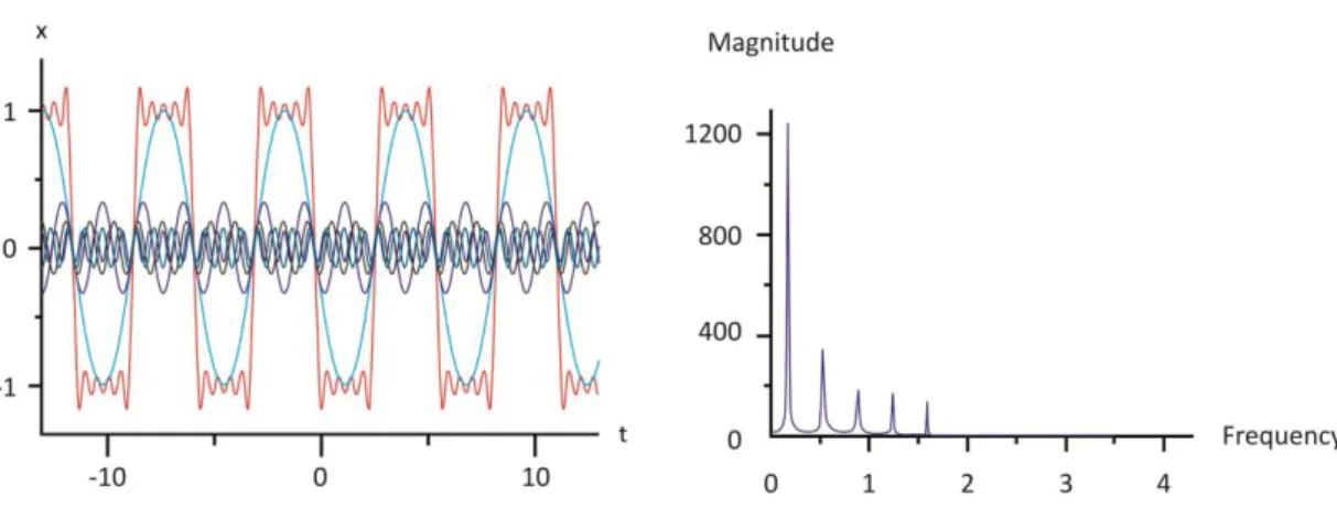
Fourier analysis supports the issue of localization in frequency. Born in the early nineteenth

cen-tury, it is the study of how functions can be approximated by sums of simpler trigonometric

functions. The Fourier transform is, thus, a mathematical transformation that converts signals

between the time domain and the frequency domain (Figure 3). The amplitudes of the signals

originate a frequency spectrum of the original function in the temporal domain.

(45)

The red curve is a periodical function which can be approximated by a sum of simple sine functions. At the right we

have the Fourier transform of the original function8_.

The main problem with the Fourier transform is that when analysing the information in the

fre-quency domain one loses the temporal information (Bloomfield 2004).

This approach allows to obtain information known as the “power spectrum” of a time series. It is also called spectral analysis. It describes how the variance of the data is distributed over the

frequencies at which the time series can be decomposed. That is, the variance distribution as a

function of the frequency range. The power spectrum is related to the auto-covariance (ACV), a

concept more easily recognized to social scientists9_{. In fact, the power spectrum contains the}

information displayed in the ACV, but in a complementary perspective because the ACV is a

function of time while the power spectrum is a function of frequency. The power spectrum may

present new information because data variability may be frequency dependent.

Spectral analysis has also been used in economics research, such as the study of business cycles,

of relations between different economic variables, military spending, the governments

popular-ity, among others (Granger 1966, Richards 1992, Gerace 2002, Wen 2005). Yet, despite its

use-fulness, it has the problem of the analysis of temporal information. Moreover, the Fourier power

spectrum analysis is only useful on stationary time series, not recommended for situations

where cycles do not have fixed periodicity (Goldstein 1988).

Wavelet analysis attempts to solve the problem of simultaneous localization in time and

fre-quency. It gives information on the amplitude of the cyclic signals, and how this amplitude varies

with time. It is a useful tool for analysing changes in the variability of data in a time series. It

8

(Source: Wikimedia commons – Fourier Transform) The red curve is a periodical function which can be approximated by a sum of simple sine functions, plotted in blue in the graphs at the centre. The right-most curve is the Fourier transform of the original function.

9_{The auto-covariance of}_𝑥

𝑡 is the covariance of x over a time-shifted value. Considering 𝐸[𝑥𝑡] = 𝜇𝑡, then

(46)

allows to decompose a time series in the time-frequency space and makes it possible to analyse

what are the main existing cycles and how these cycles are modified over time.

The theory of wavelets was developed in the 1980s and since then it has been used in various

fields, including physics, geophysics, oceanography, signal processing, harmonic analysis, and

scientific computation. Studies include the study of tropical convection, the El Niño - Southern

Oscillation, atmospheric cold fronts, the dispersion of ocean waves, wave growth and breaking

and coherent structures in turbulent flows (Torrence and Compo 1998), among many others.

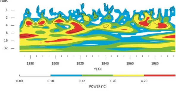
Following the previous example of Figure 2, of sea surface temperatures, below in Figure 4, we

present the respective wavelet power spectrum. In following pages, we will show how wavelet

transforms are obtained and how their tools, such as the power spectrum, are applied.

Figure 4 : Wavelet power spectrum of sea surface temperatures in the eastern Pacific

Data source: (Torrence and Compo 1998). Wavelet power spectrum of Figure 2. Black contours represent 10%

signifi-cance regions. Red areas indicate high El Niño activity.

Specifically in economics, Crowley (2007) develops a guide for wavelet use and others apply

these tools to various issues, including the decomposition of economic relationships of

expendi-ture and income (Ramsey and Lampart 1998a, b), to exchange rates (Gençay et al. 2001a, Wong

et al. 2003), monetary policy (Aguiar-Conraria et al. 2008, Rua 2012), Phillips curve (Gallegati et

al. 2011), business cycles (Baubeau and Cazelles 2009, Aguiar-Conraria and Soares 2011a,

Rita Mafalda Dionísio de Sousa