João Paulo Isidoro Ascenso
Mestrado Integrado em Engenharia Electrotécnica e de Computadores
Tool for 3D analysis and segmentation of
retinal layers in volumetric SD-OCT images
Dissertação para obtenção do Grau de
Mestre em Engenharia Electrotécnica e de Computadores
Orientador: André Damas Mora, Prof. Auxiliar, FCT-UNL
Júri:
Tool for 3D analysis and segmentation of retinal layers in
volu-metric SD-OCT images
Copyright cJoão Paulo Isidoro Ascenso, Faculdade de Ciências e Tecnologia, Universidade Nova de Lisboa
A
CKNOWLEDGEMENTS
I will start by thanking my supervisor, Professor Dr. André Mora, for the opportu-nity to develop this work and all the support given throughout its execution. The MITK and ITK community that keep the project growing and give support to all the problems developers face. To all my friends who supported me during this period and my colleges whom I had the pleasure to share the work space with and my girlfriend for always be there for me.
A
BSTRACT
With the development of optical coherence tomography in the spectral domain (SD-OCT), it is now possible to quickly acquire large volumes of images. Typically analyzed by a specialist, the processing of the images is quite slow, consisting on the manual marking of features of interest in the retina, including the deter-mination of the position and thickness of its different layers. This process is not consistent, the results are dependent on the clinician perception and do not take advantage of the technology, since the volumetric information that it currently provides is ignored.
Therefore is of medical and technological interest to make a three-dimensional and automatic processing of images resulting from OCT technology. Only then we will be able to collect all the information that these images can give us and thus improve the diagnosis and early detection of eye pathologies. In addition to the 3D analysis, it is also important to develop visualization tools for the 3D data.
This thesis proposes to apply 3D graphical processing methods to SD-OCT retinal images, in order to segment retinal layers. Also, to analyze the 3D retinal images and the segmentation results, a visualization interface that allows display-ing images in 3D and from different perspectives is proposed. The work was based on the use of the Medical Imaging Interaction Toolkit (MITK), which includes other open-source toolkits.
For this study a public database of SD-OCT retinal images will be used, con-taining about 360 volumetric images of healthy and pathological subjects.
R
ESUMO
Com o desenvolvimento da tomografia de coerência ótica no domínio espectral (SD-OCT), é hoje possível a aquisição rápida de grandes volumes de imagens. Tipicamente analisadas por um especialista da área, o processamento das mesmas é bastante lento, sendo marcadas manualmente as características de interesse na retina, nomeadamente a definição da posição e espessura das suas diferentes camadas. É ainda pouco consistente, estando em cada resultado implícita a forma de marcação e perceção dos diferentes especialistas. Além disso não tira proveito da tecnologia utilizada, que apresenta informação volumétrica que é ignorada quando feita uma análise dos cortes seccionais.
É portanto de interesse médico e tecnológico fazer um processamento tridi-mensional e automático das imagens resultantes da tecnologia OCT. Só assim se conseguirá recolher toda a informação que estas imagens nos podem dar e assim melhorar os diagnósticos e deteção prematura de doenças a nível ocular. Além da análise de características numa perspetiva 3D, é também importante a visualização dessa informação.
Este trabalho propõe aplicar métodos de processamento gráfico tridimensional em imagens da retina recolhidas através da técnica SD-OCT e desenvolver uma interface de visualização que permita apresentar as imagens em 3D e sob diferentes perspetivas. O trabalho foi baseado no uso doMedical Imaging Interaction Toolkit (MITK), que engloba vários toolkitsopensource. Para este estudo será usada uma base de dados pública de imagens SD-OCT contendo cerca de 360 imagens de indivíduos saudáveis e com patologias retinianas.
C
ONTENTS
List of Figures xv
1 Introduction 1
1.1 The retina . . . 3
1.2 Age-related Macular Degeneration . . . 4
1.3 Optical Coherence Tomography - OCT . . . 6
1.4 Toolkits . . . 8
1.4.1 The Medical Image Interaction Toolkit - MITK . . . 8
1.4.2 Insight Segmentation and Registration Toolkit - ITK . . . 9
1.4.3 Visualization Toolkit - VTK . . . 9
1.4.4 Qt . . . 9
1.5 Image Formats . . . 10
1.5.1 DICOM . . . 10
1.5.2 NRRD . . . 10
1.6 Objectives . . . 10
1.7 Thesis Structure . . . 11
2 State Of The Art 13 2.1 Noise Reduction . . . 13
2.2 Segmentation . . . 15
2.3 Volume Rendering . . . 17
2.3.1 Ray Casting . . . 17
2.3.2 Texture Mapping . . . 18
2.3.3 Other Rendering Techniques . . . 19
2.4 Surface Rendering . . . 19
3 Developed Work 21 3.1 Software Development Platform . . . 21
3.3 Noise Reduction . . . 24
3.3.1 Region of Interest . . . 24
3.3.2 Image Resample . . . 25
3.3.3 Interpolators . . . 28
3.3.4 Anisotropic Diffusion . . . 29
3.4 Segmentation . . . 30
3.4.1 Canny Edge Detection . . . 31
3.4.2 Volume Division . . . 33
3.5 Other Tools . . . 34
3.5.1 Derivative . . . 35
3.5.2 Sigmoid . . . 35
3.5.3 Gaussian Filter . . . 37
3.5.4 Mean and Median filters . . . 38
3.5.5 Flattening . . . 39
3.6 Visualization . . . 39
3.7 Prototype . . . 42
4 Results 45 4.1 Input Images . . . 45
4.2 Validation of Results . . . 46
4.3 Performance . . . 48
5 Conclusion 51 5.1 Future Work . . . 52
L
IST OF
F
IGURES
1.1 Anatomical planes. . . 3
1.2 Retinal layers observed in a microscope. . . 4
1.3 SD-OCT scan of a retina with drusen. . . 4
1.4 Macula position on the eye and detail section of retina . . . 5
1.5 Retinal fundus photography showing drusen. . . 5
1.6 Image quality of time domain and spectral domain OCT . . . 6
1.7 Comparison between the two acquisition techniques . . . 7
1.8 OCT scanning schematic. . . 8
1.9 Relation of MITK to the toolkits ITK, VTK and Qt . . . 9
2.1 RMS error for recovering a noisy image. . . 14
2.2 Example of the resulting segmentation from Garvin et al. (2009). . . 16
2.3 Example of the resulting segmentation of 7 layers from a pathological eye 17 2.4 Resulting segmentation of 11 layers by Kafieh et al. (2013b) . . . 17
2.5 Example of the four ray traversal methods . . . 18
2.6 Triangulated Cubes . . . 20
3.1 CMake configuration window. . . 22
3.2 Example images from the used dataset. . . 23
3.3 Diagram for the noise reduction process. . . 24
3.4 Process for extracting the ROI . . . 24
3.5 Example of the noise reduction pipeline. . . 26
3.6 Comparison of an image with different resolutions. . . 27
3.7 Impact of upsampling the number of slices in the volume. . . 27
3.8 Example of the different interpolation techniques . . . 29
3.9 Comparison between the two diffusion methods . . . 30
3.10 Segmentation process diagram . . . 31
3.11 Canny filter’s output on anisotropic and isotropic data . . . 32
3.13 Steps to upsampling the segmentation. . . 33
3.14 Example of thresholds selected by different methods. . . 34
3.15 Output of the sigmoid filter withα=10 andβ= 190. . . 36
3.16 Plot of sigmoid function with different parameters . . . 37
3.17 Example of the Gaussian filter’s output . . . 38
3.18 Comparison between mean and median filters . . . 38
3.19 Rendering of flatten volume . . . 39
3.20 Different rendering modes . . . 40
3.21 Rendering of Canny filter’s output without flattening. . . 41
3.22 Graphic User Interface . . . 42
4.1 Segmentation of the three target surfaces on resampled volume. . . 47
G
LOSSARY
Anisotropic An object having a physical property that has a different value when measured in different directions. .
ARMD Age-related Macular Degeneration. CSV Comma-Separated Values.
DICOM Digital Imaging and Communications in Medicine. DOCTRAP Duke OCT Retinal Analysis Program.
GCL Ganglion Cell Layer. GPU Graphics Processing Unit. ILM Inner Limiting Membrane. INL Inner Nuclear Layer. IPL Inner Plexiform Layer. IS Inner Segment.
ITK Insight Segmentation and Registration Toolkit. MCDE modified curvature diffusion equation. MITK Medical Image Interaction Toolkit. MOC Meta-Object Compiler.
NFL Nerve Fiver Layer.
ONL Outer Nuclear Layer. OPL Outer Plexiform Layer. OS Outer Segment.
RMS root mean square. ROI region of interest.
C
H A P T E R1
I
NTRODUCTION
Image is a valuable tool in medicine providing the means for a noninvasive mapping of a subject’s anatomy. Magnetic resonance imaging (MRI), digital mam-mography and computed tomam-mography (CT), are a few examples of technologies that have improved the knowledge of the anatomy for medical research, diagnosis and treatment planning (Pham et al., 2000)
Being in constant use in modern medicine, the large amount of the generated images brings the need for computers to help with their processing and analy-sis. The time spent by specialists delineating regions of interest and anatomical structures urges the development of computer algorithms that can perform the same task automatically, with high precision and reproducibility. This is possible with the application of segmentation methods that extract meaningful informa-tion from the image and facilitate their display in a clinically relevant way. To better understand this information a visual representation is often needed. The visualization of medical data includes a way to interact, process and represent the data. The visualization process begins by acquiring the data, processing it with the application of noise reduction and feature extraction methods for instance, and lastly the data is rendered or displayed.
and manual intervention as well. With the production of quality 3D information, methods to use it in segmentation and visualization must be developed.
Classically, image segmentation is defined as the partitioning of an image into non-overlapping, constituent regions that are homogeneous with respect to some feature such as intensity or texture (Pal and Pal, 1993). Only recently OCT image segmentation has a more dedicated research and remains one of the most difficult and required step in OCT image analysis, because there is no universal segmentation method that will deliver good results in different situations.
Having 3D information available, it is important to make the best use of it to follow the evolution of the acquisition systems. Three-dimensional medical images were usually analyzed as sequences of 2D slices, which lacks contextual information between slices. Performing segmentation in 3D space will give more consistent results, defining object surfaces rather than sets of individual contours.
A correct intraretinal segmentation is an important tool for ophthalmologist to better understand and study pathologies. Several applications of the segmentation can be defined, like volumetric measurements of the scan in defined regions, comparison of retinal thickness during treatment and detection of pathologies that affect the thickness of retinal layers, among others.
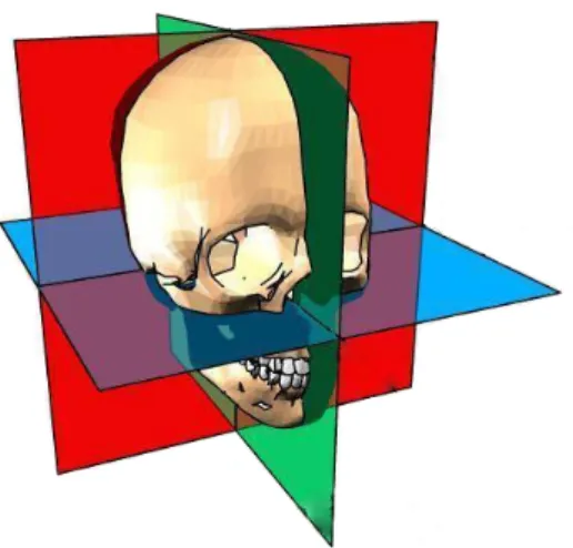
The objective of this work is to explore methods of volumetric processing of OCT images in order to identify retinal layers, as well as to develop an interface that enables viewing and interaction with such data. The 3D image can be sliced in any direction but is typically viewed along the anatomical planes. This planes are named axial, sagittal and coronal, being the(x,y),(y,z)and(x,z)Cartesian planes, respectively. Figure 1.1 shows the position of each plane relative to the human skull.
This nomenclature is used along the present work and the images shown in this document relate to this planes. Note that they are a slice of the volume and not an isolated 2D image, so they are representative of the 3D processing results.
1.1. THE RETINA
Figure 1.1: Anatomical planes. Axial plane in blue, sagittal in green and coronal in red. Adapted from Anatomia Online (2014)
1.1
The retina
Is important to start by introducing the retinal structure to better understand what is seen in the OCT scans.
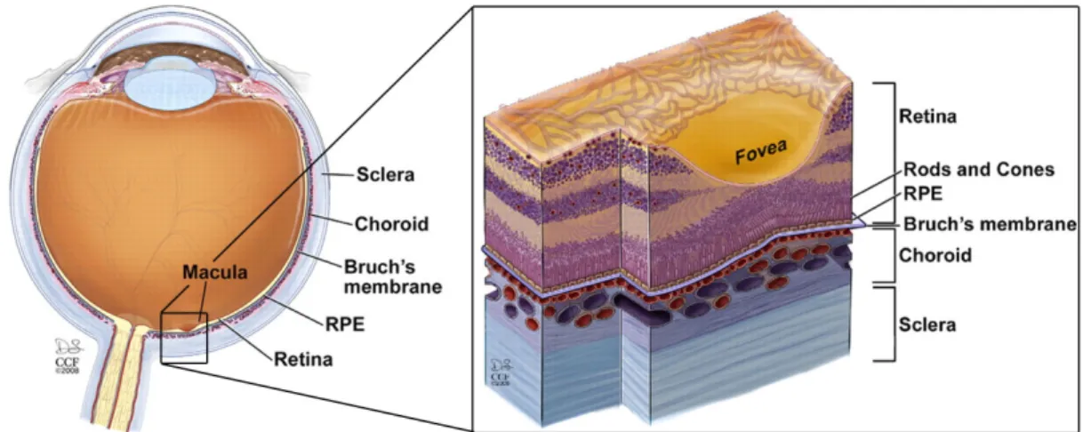
The retina covers the back of the eye in about 65% of its interior surface. It is responsible to convert the light into signals that are sent to the brain, through the optic nerve. In the middle of the retina a small dimple is found named as fovea. This spot is where the eye has the most color perception and where vision is sharpest. The fovea is the central point in a depression that goes from 2.5 to 3mm in diameter known as macula. All the studied OCT scans are from this region of the retina, identified in figure 1.4.
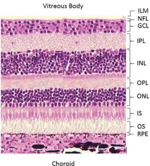
As represented in the figure 1.2 its structure shows different layers. From the inside to the outside of the eye, the first surface detectable is the limit between the vitreous and the retina. The choroid is the vascular layer of the eye and lies behind the retina. The nomenclature used throughout the document and shown in the figure are as follow:
• Inner Limiting Membrane (ILM) • Nerve Fiver Layer (NFL)
• Ganglion Cell Layer (GCL) • Inner Plexiform Layer (IPL) • Inner Nuclear Layer (INL)
• Outer Plexiform Layer (OPL) • Outer Nuclear Layer (ONL) • Inner Segment (IS)
• Outer Segment (OS)
Figure 1.2: Retinal layers observed in a microscope. Adapted from Bristol Univer-sity (2000).
1.2
Age-related Macular Degeneration
According to the World Health Organization (2007), Age-related Macular Degener-ation (ARMD) is the leading cause of blindness in the developed world. Usually it produces a slow, painless loss of vision. Ophthalmologists often detect early signs of macular degeneration, before anomalies are detected in a retinal exam.
Figure 1.3: SD-OCT scan of a retina with drusen.
1.2. AGE-RELATED MACULAR DEGENERATION
Figure 1.4: Macula position on the eye and detail section of retina (Yuan et al., 2010).
It is possible to observe the retina by photographing it directly through the pupil. This method is called fundus photography (figure 1.5) and is used to di-agnose and treat eye diseases. These images are commonly used to follow the development of drusen. Similar to OCT images, the evaluation of this images can be fastidious when done manually, not ensuring coherent results. To solve such problems some automatic classification techniques have also been developed in these type of images. Smith et al. (2005) used the Otsu method to identify drusen after some pre-processing of the image. Mora et al. (2011) presented an automatic drusen detection that achieves similar results to the experts and with a higher reproducibility, using a gradient based segmentation algorithm.
1.3
Optical Coherence Tomography - OCT
OCT is a powerful imaging system that produces images based on interference patterns. The development in OCT technology has enable to acquire more data and faster, reaching resolutions in theµm level and penetration of a few millimeters in scattering media. It has been widely used from material inspection to medical imaging and is very common in the ophthalmology field.
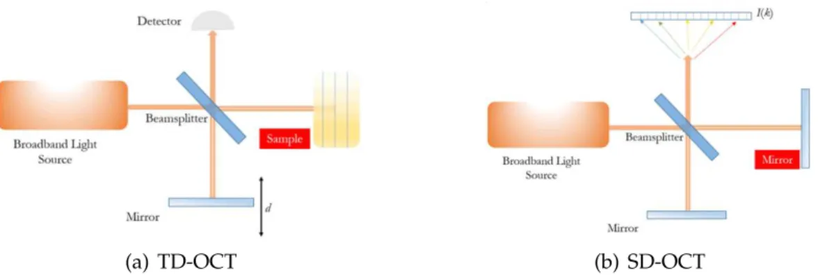
An early version of this technology, Time Domain OCT (TD-OCT), has a mov-ing reference mirror and uses low-coherence interferometry as an indirect measure of the time of travel of the light reflected in the sample. In low-coherence interfer-ometers a light beam is emitted by a source with a broad optical bandwidth and split into two different paths, known as reference and sample arms of the interfer-ometer, reaching then a mirror and the subject to be imaged respectively (figure 1.7(a)). As the mirror moves, the reflected light from each path is guided into a photo-detector, that records the light intensity and analyses the interference effect, used as a relative measure of distance traveled by the light beam. This interference pattern appears when the mirror is nearly at the same distance as the reflecting structure in the sample. The displacement distance of the mirror between the occurrence of interference is the optical distance between two reflecting structures. In case of the retina, it contains layers with different reflection indexes, and the transition between layers causes intensity peaks in the interference pattern. Being a mechanical process, it is relatively slow and limits both the amount of data that can be captured and the image quality.
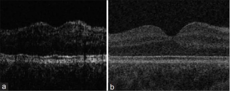
Figure 1.6: Image quality of time domain (a) and spectral domain (b) OCT (Kafieh et al., 2013a)
1.3. OPTICAL COHERENCE TOMOGRAPHY - OCT
problems and limitations of the TD-OCT system. A comparison between the outputs of the two modalities can be seen in figure 1.6. It does not have any moving parts (the reference mirror is fixed), which enables faster acquisition times and higher density. The detection system is now a spectrometer, where intensity is recorded as a function of the light frequency. The resulting intensity modulations are named spectral interference. Each reflecting layer has a different location in the sample, represented by the rate of intensity variation over different frequencies (Wasatch Photonics, 2015).
(a) TD-OCT (b) SD-OCT
Figure 1.7: Comparison between the two acquisition techniques (Wasatch Photon-ics, 2015)
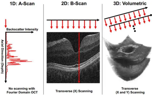
As the light beam hits the sample, its reflection gives information on that particular position, producing an A-scan.
As presented in 1.8, the A-scan is a one dimensional acquisition, that measures the intensity of light back-scattered for different depths in the axial direction. A B-scan is a 2D image obtained by translating acquisition of A-scans in a transverse direction. For last the volumetric scan is a sequence of B-scans, where each one is a slice of the volume in a given position.
Figure 1.8: OCT scanning schematic (Kraus et al., 1991).
1.4
Toolkits
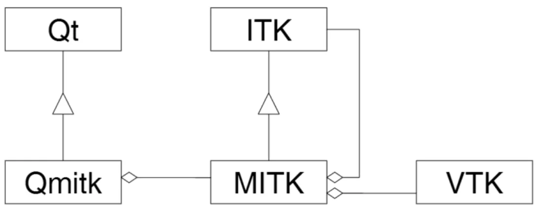
The development of the proposed application relies on the usage of volumetric visualization and processing toolkits, the Visualization Toolkit (VTK) and the Insight Segmentation and Registration Toolkit (ITK) respectively, which are fre-quently used in 3D medical image visualization. These are currently maintained by Kitware, Inc., a company dedicated to the development and support of open-source software. To integrate both toolkits the Medical Image Interaction Toolkit (MITK) was used, a framework maintained by the German Cancer Research Cen-ter, presented below. MITK relies on Qt to provide a dynamic interface. How these toolkits are related can be better understood with the class diagram in figure 1.9. Qmitk is a helper class that merges the high interactivity of MITK with the graphic interface possibilities provided by Qt.
1.4.1
The Medical Image Interaction Toolkit - MITK
1.4. TOOLKITS
of medical imaging software with a high degree of interaction, making it a consis-tent framework to combine image segmentation, registration and visualization. It combines VTK and ITK and adds important features for developing interactive medical imaging software and that are not covered by any of the others.
Figure 1.9: Relation of MITK to the toolkits ITK, VTK and Qt
1.4.2
Insight Segmentation and Registration Toolkit - ITK
The ITK is a large and complex open-source software toolkit for performance of im-age registration and segmentation. Its implementation in C++ employs generic pro-gramming, using templates, allowing that many of the algorithms can be applied to arbitrary spatial dimensions and pixel types (Johnson and Mccormick, 2014).
1.4.3
Visualization Toolkit - VTK
The Visualization Toolkit is an open-source software system for 3D computer graphics, image processing, and visualization. It is a C++ class library that sup-ports a wide variety of visualization algorithms, as well as advanced modeling techniques and offers some 3D interaction widgets. The toolkit supports paral-lel processing and integrates with various databases on GUI toolkits such as Qt. VTK is used in commercial applications, as well as in research and development (Kitware, 2016).
1.4.4
Qt
open-source. It uses a preprocessor, the Meta-Object Compiler (MOC), to extend the C++ language, including features like signals and slots that connect elements of the interface. The graphic user interface in MITK is based in by this framework (Qt, 2015).
1.5
Image Formats
When working with large set of images, some standards are more helpful in man-aging the files. In the medical field, information about the patient and acquisition conditions are important to keep along with the data that is transferred between medical staff and hospitals.
Below are the two standards used in this project, both allow easy storage and management of the 3D data sets.
1.5.1
DICOM
Digital Imaging and Communications in Medicine (DICOM) is the international standard that defines a set of norms for processing, storage, transmission and displaying of medical images as well as derived structured documents (ISO 12052). Created to ensure the interoperability between systems, it allows products to work with present and future imaging modalities, regardless of the vendor.
Used in hospitals worldwide, it is implemented in many imaging devices in fields like radiology, cardiology imaging, radiotherapy, dentistry, ophthalmology and more (NEMA, 2016).
1.5.2
NRRD
Nearly Raw Raster Data (NRRD) it is a library and file format intended to sup-port scientific visualization and image processing applications. It works with N-dimensional raster data and is flexible with the type, encoding and endianness. The library also supports PNG, PPM, PGM and some VTK datasets (NRRD, 2016).
1.6
Objectives
1.7. THESIS STRUCTURE
developed a visualization interface, with views from different perspectives and 3D models.
1.7
Thesis Structure
This thesis is divided into five chapters organized using the following structure. On Chapter 2 is presented the state of the art, focusing on previous solutions for the segmentation of OCT images. One of the main problems when dealing with this images is their significant noise, therefore most commonly used methods for noise reduction are presented. On the segmentation techniques, the newest methods and a reference to the older one are presented. Then a brief explanation on surface and volume rendering is given.
Chapter 3 presents all the developed work and methods applied. Going through all the process of segmentation from noise reduction to presentation of the results. In the end of this chapter the developed prototype is presented with an explanation of its basic functionalities.
On Chapter 4 a comparison and validation of the proposed segmentation is made. Using the manual segmentation available it is possible to compare the algorithm to it and evaluate the segmentation error. The results obtained are then compared to the ones presented in previous publications.
C
H
A
P
T
E
R
2
S
TATE
O
F
T
HE
A
RT
In this chapter the methods that achieve the best results in the processing of retinal OCT images and the most advanced image processing techniques in 3D will be presented. The main challenges are related to noise reduction and efficient and robust segmentation. A recent overview of the techniques that face these problems was made by Baghaie et al. (2014), and also includes a chapter on image registration. Besides the image processing, is essential to display the data and results graphically to better understand them. An overview of visualization of 3D data is made in the last sub-chapter.
2.1
Noise Reduction
One of the characteristics of images acquired by narrow band systems like OCT is the presence of speckle noise that reduces contrast and degrades the image in a way that makes detecting the retinal layers a difficult task. This type of granular noise is influenced by backscattering of the beam inside and outside of the sample volume and random propagation delays caused forward scattering. These scattered signals add coherently, creating regions of constructive and destructive interference, that appear as speckle noise in the image (Schmitt et al., 1999).
Noise reduction techniques can be applied during data acquisition, being the compounding techniques one effective way to reduce the speckle noise. These techniques are divided into four main categories: spatial-compounding (Avanaki et al., 2013), angular-compounding (Schmitt, 1997), frequency-compounding (Pircher et al., 2003) and strain-compounding (Kennedy et al., 2010). These compounding methods are usually not preferred since they require multiple scans of the same data. They rely on changing the OCT system with the drawback of increasing the system complexity. Therefore, the use of post-processing techniques is more popular.
The well-known anisotropic diffusion method proposed by Perona and Ma-lik (1990) is used for speckle reduction. The ability in preserving edge information is what makes this filter so popular.
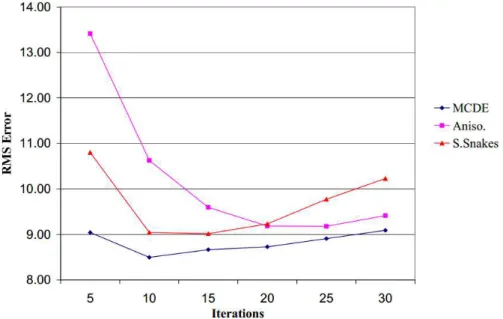
Different variations of it have been made, one of them is the Modified Curva-ture Anisotropic Diffusion. This method, proposed by Whitaker and Xue (2001) has shown to be more effective than the classic anisotropic diffusion at removing noise, being more aggressive at enhancing edges and less sensitive to contrast. It is based on a level-set equivalent of the equation proposed by Perona and Malik (1990) named modified curvature diffusion equation (MCDE).
The figure 2.1 shows the root mean square (RMS) error as function of the number of iterations of the filter, and confirms the better performance of the MCDE filter.
2.2. SEGMENTATION
Salinas and Fernández (2007) compare the one other variation, the complex diffusion filter proposed by Gilboa et al. (2004) with the traditional Perona-Malik filter, which resulted in better speckle noise removal.
Wavelet transform has also been used and showed promising results, but its lack of directionality imposes a limitation on proper denoising images. Other methods using median filters, mean filters, directional filtering, low-pass filtering or 2D smoothing, among others, can be found in literature.
2.2
Segmentation
Being one of the most difficult steps in OCT image analysis, segmentation is also the most required. During the last two decades several of methods were proposed. Besides the presence of noise covered in the previous section, other problems are encountered in the segmentation of OCT images (Baghaie et al., 2014) like the variation of intensity within the same layers. Also the shadows caused by blood vessels create holes in the segmented surfaces what affects the performance of the segmentation methods. Finally, the relative motion of the subject, even from breathing or the heart beat, causes motion artifacts that degrade the image.
A typical approach for segmenting retinal layers consist on preprocess the image (with median filter or anisotropic diffusion per example), find features of interest on each A-scan and in some cases correct their discontinuities.
The retinal segmentation methods can be categorized into five classes:
• methods applicable to A-scans; • intensity-based B-scans analysis; • active contour approaches;
• analysis methods using artificial intelligence and pattern recognition
tech-niques;
• segmentation methods using 2D/3D graphs constructed from the 2D/3D
OCT images.
The method proposed in this work can be classified as a 3D intensity-based solu-tion. Kafieh et al. (2013a) presented a in depth study of segmentation algorithms used in segmentation of the retina. For the purpose of this study more focus will be given to 3D approaches.
Sun and Zhang (2012) proposed a 3D method based on pixel intensity, bound-ary information and intensity changes on both sides of the layer simultaneously, which can segment the RPE, IS/OS and ILM layer boundaries.
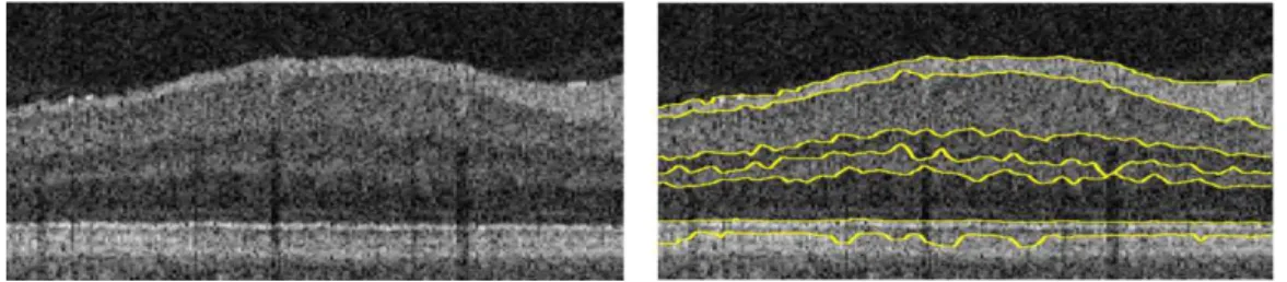
Figure 2.2: Example of the resulting segmentation from Garvin et al. (2009).
One of the most promising techniques in image segmentation uses the theory of graphs (Li et al., 2006). An algorithm proposed by Garvin et al. (2008) trans-forms a 3D segmentation problem into finding a minimum cost closed set in a vertex-weighted geometric graph. This graph is created from edge and regional image information as well as a definition of surface interaction and smoothness constraints that evaluate the feasibility of a surface. This method guarantees to find the optimal solution with respect to the cost function defined. A similar method as been applied by Chiu et al. (2010), with results seen in figure 2.3, but in a 2D approach and combining dynamic programming what reduced the processing time. Here each B-scan is represented as a graph of nodes and each node corre-sponds to a pixel that connects to others by links referred as edges. To precisely cut the graph is essential to assign the appropriate edge weights, using metrics as distance between pixels or intensity differences. Finally, the Dijkstra’s algorithm is used as an efficient way to find the lowest weighted path on the graph.
Using support vector machines, graph theory, and dynamic programming, Srinivasan et al. (2014) also achieves an accurate segmentation of seven to ten layers.
Niemeijer et al. (2008) developed a method to segment blood vessels in 3D SD-OCT images of the retina, processing the volume slice-by-slice.
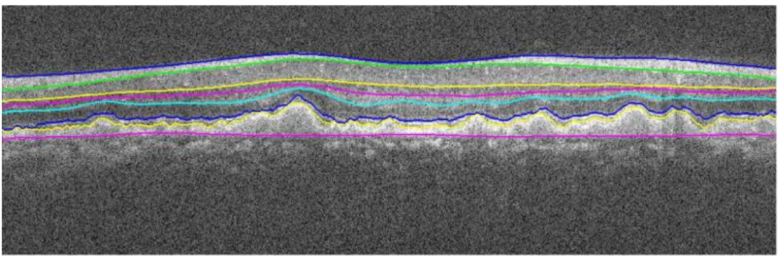
Another recent approach was the use of diffusion maps by Kafieh et al. (2013b) what instead of using edge-based information, relies on regional image texture, improving the robustness of the segmentation of low contrast or poor inter-layer gradients cases (figure 2.4). This method can be applied in both 2D and 3D data, presenting better results when detecting the layers position in 3D.
2.3. VOLUME RENDERING
These two processes can’t be completely separated (Zhou and Tönnies, 2003). Without visualization, the segmentation results can’t be presented.
Figure 2.3: Example of the resulting segmentation of 7 layers from a pathological eye by Chiu et al. (2010).
Figure 2.4: Resulting segmentation of 11 layers by Kafieh et al. (2013b)
2.3
Volume Rendering
Medical images are often acquired in a set of 2D images, equally spaced between them, which allows their rendering as a volume. Volume rendering, also referred as direct volume rendering or composite rendering, is based on the simulation of light passing through matter with the objective of displaying a 3D image in its entirely (Papademetris and Joshi, 2009). Volume rendering gives better image quality and doesn’t define surfaces when generating images. On the down side, since it uses all the voxels of the image, the execution time is proportional to the size of the dataset.
2.3.1
Ray Casting
values are defined by transfer functions that adjust the rendering output in order to get desired results. The classic technique known as ray casting, was introduced by Levoy (1988). He defined the following equations which are executed at every point along the ray:
Ci+1= Ai∗Ci+ (1−Ai)∗ai∗ci (2.1) Ai+1 = Ai+ (1−Ai)∗ai (2.2) whereCi stands for the accumulated color along the ray and Ai represents the accumulated opacity along the ray. The current voxel’s color and opacity, which is obtained from the transfer function, is respectivelyciandai. Every time the ray hits a non-zero voxel, the color and opacity are looked up in the transfer function. There are different ray traversal methods. In the most basic, known as first-hit, the first non-zero voxel found is used to map the volume. The average method computes the average of the voxels’s intensity. The Maximum Intensity Projection (MIP), uses the maximum intensity found across the ray. The most common method is called Accumulate. Here the color and opacity are accumulated along the ray path allowing to display multiple surfaces, like skin and bone on the same volume. An example of the resulting volume from each method can be seen in figure 2.5.
Figure 2.5: Example of the four ray traversal methods. Fist-hit, Average, MIP and Accumulate (Papademetris and Joshi, 2009)
2.3.2
Texture Mapping
2.4. SURFACE RENDERING
Three-dimensional texture mapping however allows the data to be loaded into a single 3D texture. Slices are then made parallel to the viewing direction, simulating trilinear interpolation, and since a single data structure is used there is no need to have 3 copies of the same data, saving memory.
2.3.3
Other Rendering Techniques
Other techniques like Shear Warp proposed by Lacroute and Levoy (1994) and Splatting proposed by Westover (1990) are also important. Shear warp is recog-nized as one of the fastest rendering methods, but sacrifices the image quality. Based on three steps, the algorithm starts by shearing and resampling the volume slices, then projects an intermediate image that is finally warped into the final image.
In Splatting techniques the volume is represented by a field of 3D kernels with amplitudes related to the voxel’s intensity. The name comes from the similarity to throwing a snowball against a wall. Each kernel leaves a weighted footprint that will accumulate into a image.
A deeper explanation and comparison between the most used volume render-ing algorithms is made by Zhou and Tönnies (2003).
2.4
Surface Rendering
Unlike volume rendering, surface rendering aims to represent only some features from the total volume, representing boundaries of a structure. The resulting surface is called an isosurface and each surface has a unique value known as iso-value.
C
H
A
P
T
E
R
3
D
EVELOPED
W
ORK
This chapter presents the overall pipeline for the image processing and the meth-ods applied. To implement image processing and visualization tools, the search for the best platform lead to VTK as a popular toolkit for medical image visual-ization with strong support for 3D data. The following sub chapter presents the challenges faced on using this platform. Then will be presented the steps towards noise reduction, layer segmentation and the graphical user interface prototype.
All 2D images presented throughout the document show slices of the volume in the axial plane,(x,y), unless referenced otherwise. Similar images are used for
easy comparability of results from the various filters applied. In binary images the color was inverted to get a clearer visualization when printed. Often the term pixel is used when presenting a slice of the volume, but since all the processing is done with the volume, pixel often refers to voxel.
3.1
Software Development Platform
Initially the software was intended to be developed in C# language. The search for the best toolkit for image processing and 3D visualization lead to ITK and VTK, respectively. Even though these are implemented in C++, a few wrappers are available including for C#, named ActiViz.NET and SimpleITK, for VTK and ITK respectively.
since VTK by itself has limited image filtering capabilities. This brought a problem in interconnecting this two wrappers. Even though the basic data being analyzed is the same, each one was its own image type definitions and are not directly interchangeable. A solution was found but incompatibilities kept emerging with further developments what lead to the decision of changing the programming language and start using the toolkits’ native one.
This initial effort was helpful by the knowledge gathered about the toolkits, but ended up not having any usage on the final solution. The time spent on this issues delayed the development of the solution.
The work was then developed in C++ using the MITK toolkit, which integrates ITK (v4.7) with VTK (v6.2) and uses the Qt framework for the GUI. It is important to note the size of these toolkits, that can take several hours to build, and their configuration might bring some problems besides the documentation available. The setup of the toolkits was difficult and took some time to make them work without problems.
Figure 3.1: CMake configuration window.
3.2. INPUT IMAGES
of all the toolkit at once, but to build some features that are not default in this template, ITK and VTK must be build separately in order to access and enable those tools. An Open-GL enabled Qt version must be installed previously. After the configuration is done, the project template is build in either Debug or Release configuration. This builds MITK and all its dependencies. In this project, template is not used in the development since we are building our own application outside of the MITK framework, so a new project is started. An helpful guide1is available for configuration but some issues may occur that will need closer attention. Is recommended to test the available examples in order to get familar with the toolkit.
3.2
Input Images
This thesis worked with the OCT retinal image dataset available from Duke University (Farsiu et al., 2014). This dataset presents images from healthy and patological subjects, as seen in figure 3.2, but on this stage we focus only on healthy retinal images. Volumetric scans (6.7 x 6.7mm) were acquired from normal adult subjects using Bioptigen, Inc. SD-OCT imaging systems. The scan is composed by 100 slices. Each slice is a B-Scan and correspond to the(x,y)plane, with a size of 1000 x 512 pixels. The pixel sampling spacing, is 6.7µm lateral (1000 A-scans) and 67µm in the azimuthal direction (100 B-scans). The number of A-scans represents the image width.
(a) Image of healthy retina (b) Image of retina with drusen
Figure 3.2: Example images from the used dataset.
1www.mitk.org/wiki/Developer
3.3
Noise Reduction
Before any segmentation there is the need to reduce the speckle noise present in the volume. The figure 3.3 resumes the steps taken. The first one is to extract the volume’s region of interest (ROI) in order to remove regions that do not present any useful information. Then the volume is downsampled in a pyramidal approach to half its size. Having considerably reduced the volume size, it is applied an anisotropic diffusion filter to decrease the speckle noise. Lastly, before any further segmentation is important to resample the volume, in order to become isotropic. This sub-chapter explores each step of this process.
Figure 3.3: Diagram for the noise reduction process.
3.3.1
Region of Interest
In order to reduce the computation time it is important to ignore parts of the volume that don’t give any relevant information. In the OCT scans, the area above the first layer of the retina and below the last one are useless to the segmentation process and cover a big part of the image. So these areas of the image are cropped, reducing memory usage and computation time. It is important to note that the position of the retina in the OCT scan can change through the 100 B-scans available. To face that, the process starts by projecting the volume into one slice, keeping the maximum pixel value along the several B-scans (figure 3.4(a)). This way it is possible to get the coordinates where there is information across the volume.
(a) Max. Projection (b) Binarization
3.3. NOISE REDUCTION
Having one slice with the maximums projection (figure 3.4(b)), a mean filter with a horizontal kernel of 5x1 pixels is applied to remove isolated points away from the ROI, that might be selected by the subsequent binarization, and to fill the gaps inside the ROI. The binarization of the image allows to easily find the top and bottom coordinates of the ROI and select the volume of interest, as shown is figure 3.4(b). It is used a threshold of 140, setting the inside value as white (255) and the outside as black (0). This threshold was determined empirically and shown to be suitable for the data set in study.
The total volume is then cropped in they-axis, keeping the volume in between the two found coordinates (figure 3.5(a)). Cropping the ROI reduces almost to one half of the image size and it will speed up significantly the following noise reduction and segmentation steps.
3.3.2
Image Resample
With the objective of reducing memory, computation time and image noise, a downsampling of the image using a pyramidal approach is performed. This method allows the creation of an pyramidal image according to a predefined multi-resolution configuration. This configuration is specified in terms of shrink factors for each multi-resolution level and for each dimension.
A shrink factor of 2 was defined, downsampling the volume to half its size in all dimensions (figure 3.5(b)). To achieve it two computation levels are defined, having the last one a neutral shrink value of 1, demanded by the filter in use. To generate each output image, a Gaussian smoothing is first applied with the variance set to (shrink f actor/2)2. The smoothed image is then downsampled
using the ITK’s ResampleImageFilter. This filter resamples an existing image through a identity coordinate transform, interpolating with a linear function. Output information such as spacing, size and direction for the output image should be set. A recursive version of this filter is used since it is about 60% faster than the non-recursive one. This step allows the following anisotropic diffusion filter to perform in reasonable time. The volume should not be downsampled in thez-axis since it is already subsampled relative to the(x,y)plane resolution, but
without doing it the next step takes more than 4 minutes to perform. In future implementations of the anisotropic diffusion filter in the Graphics Processing Unit (GPU), the z-axis downsampling should not be done.
(a) Full size ROI
(b) ROI downsample to half of its size
(c) Output of the speckle diffusion filter
(d) Resampled to be isotropic
Figure 3.5: Example of the noise reduction pipeline.
3.3. NOISE REDUCTION
(a) (b)
Figure 3.6: Comparison of an image with different resolutions. Downsampled by a factor of 2 (a) and by a factor of 4 (b)
It was decided to reduce the image by a factor of 2 in the pyramidal downsam-pling, since a higher reduction would degrade features in the image. A comparison is made in figure 3.6. Decreasing the resolution by a factor of 4 makes the pixels bigger and the segmentation becomes too coarse, with large flat segments that don’t give an accurate representation of the original surfaces. However, when resampling the image to become isotropic, the best relation between losing infor-mation in the(x,y)plane and the creation of new slices due to interpolation must be found.
To keep the 1000px width it will mean to turn each slice into 10. This large interpolation loses image features and results in poor segmentation. Keeping the downsampled width of 500pxstill shows some artifacts in the segmentation and increases the number of pixels 2.5 times, slowing all the process.
A size of 316px for the x and z-axis was a reasonable solution. It does not increase the total number of pixels and keeps the features of interest (figure 3.5(d). This value is obtained by the geometrical mean between the width and depth of the original volume (√1000∗100=316). The figure 3.7 compares the sagittal plane before and after upsampling the number of slices
(a) Sagittal plane image detail with
origi-nal spacing. (b) Sagittal plane image detail after up-sampling
3.3.3
Interpolators
The resampling of an image requires interpolation between the points, what can be done using different methods. The chosen interpolation method affects the quality of the resampling and the computation time. More complex interpolation provides better results, with the downside of longer computation times. Hence a balance between time and complexity when choosing the interpolation scheme must be made.
ITK provides nearest neighbor, linear, B-spline and window sinc interpolators (figure 3.8). The most basic one is the nearest neighbor interpolation, which simply uses the intensity of the closest pixels. Linear interpolation assumes a linear inten-sity variation between image positions and produces a continuous interpolation in space.
When interpolating with B-spline function, coefficients are computed using recursive filtering. A B-spline of order n is a piecewise polynomial function of degree<nin a variablex. ITK implementation supports splines of order from 0
to 5.
The windowed sinc interpolation is the best method for discrete data. Based on a Fourier analysis this method delivers the more precise interpolation, con-volving the spatial discrete signal with a sinc function. However, it result in long computation times.
3.3. NOISE REDUCTION
(a) Neares Neighbor
(Wikipedia, 2007b) (b) Linear (Wikipedia (2007a))
(c) B-spline. Adapted from
Technische Universitat
München (2010)
(d) Windowed Sinc. Adapted from Wikipedia (2013)
Figure 3.8: Example of the different interpolation techniques applied to a set of points.
3.3.4
Anisotropic Diffusion
OCT images are commonly contaminated with speckle noise. Anisotropic diffusion methods are formulated to reduce noise in images while preserving image edges. A 3D version of the classic Perona and Malik (1990) anisotropic diffusion equation for scalar-valued images was applied in this work.
Two variations of this filter were tested, one using a modified curvature diffu-sion equation (MCDE) and another using a gradient magnitude based equation, both available in ITK. In figure 3.9 a detail of the same image after the application of both the anisotropic diffusion methods, shows the better edge preservation with the MCDE filter. Both images have been downsampled before.
(a) Example of image before filtering
(b) Filtered with MCDE (c) Filtered with Gradient Diffusion
Figure 3.9: Comparison between the two diffusion methods
3.4
Segmentation
Being the present thesis a follow up on the work done by Coelho (2015) that uses the Canny filter as main technique for segmentation, here the same method is also used to understand the impact of the volumetric information on its results.
Initially in this work, segmentation was achieved through manipulation of intensities and binarization, but was not suitable for all cases. A graph-cut ap-proach was considered and a basic algorithm was tested, but the complexity of the implementation and the time available to explore it force to abandon the idea.
3.4. SEGMENTATION
from a bright to a dark layer or vice-versa. In this case, is known that the RPE-Choroid is a bright to dark transition and so the derivative is negative. In some cases the RPE-Choroid surface is located using a sigmoid filter, presented in section 3.5.2, to enhance the RPE layer and segment it with the Canny filter.
Figure 3.10: Diagram of the process for segmentation of three surfaces of retinal layers .
3.4.1
Canny Edge Detection
Canny (1986) defined in his paper three criteria to evaluate the performance of an edge detection filter: good detection, with low probability of marking false edges or failing to mark real edges; good localization, points marked must be close to the center of the real edge and no multiple detection of the same edge. With this definition he developed an optimal layer detection method know by his name. The ITK implementation of this filter for 3D scalar-valued images was used to detect the surfaces between the retinal layers.
The Canny filter is based on the following steps: 1. Smooth the input image with a Gaussian filter;
2. Calculate the second directional derivatives of the smoothed image;
3. Non-Maximum Suppression: the zero-crossings of second derivative are found, and the sign of the third derivative is used to find the correct extrema; 4. The hysteresis thresholding is applied to the gradient magnitude (multiplied
with zero-crossings) of the smoothed image to find and link edges. It is recommended a upper to lower ratio between 2:1 to 3:1.
Before applying the canny filter the image is resized to become isotropic, with the same pixel spacing in all directions. The image to be then processed has a size of 316 xyx 316 pixels, beingydependent of the ROI’s height. This is a solution to eliminate the original distance between slices and remove artifacts that result when the slices are not align.
The results from the canny filter can be compared in figure 3.11. Here the original spacing between slices originated an output with thick edges, instead of the expected one pixel wide edge as seen in figure 3.21(b).
(a) Image(x,y,z)with size 500x117x50 pxand spacing of 0.0134, 0.0134 and 0.134mm
respectively.
(b) Image(x,y,z)with size 500x117x500pxand spacing of 0.0134mmin all dimensions.
Figure 3.11: Canny filter’s output on anisotropic (a) and isotropic (b) data with same threshold.
Since the segmentation is done in a downsampled isotropic approximation of the original, after the filter it should be resampled to the initial size. Being the output a binary image, aliasing effects appear and the segmentation fails to follow the real edge of the segmented layer. An anti-aliasing filter should be applied before upsampling to maintain the proper segmentation.
Figure 3.12 shows the impact of this filter in the resulting upsampled segmen-tation. In the section 3.6 more focus is given to aliasing effects.
3.4. SEGMENTATION
(a) Without anti-aliasing filter (b) With anti-aliasing filter
Figure 3.12: Detail of the upsampled segmentation result.
resulting in what is seen in fig. 3.13(c). An average filter is later applied in MATLAB to eliminate the coarse appearance of the segmentation.
(a) Upsampled to original size (b) Dilatation
(c) Non-maximum suppression
Figure 3.13: Steps to upsampling the segmentation.
3.4.2
Volume Division
One of the problems faced when using the canny filter is that the retinal layers do not have a constant intensity and contrast along theirx-axis, and since canny is dependent on that contrast, it is difficult to find a threshold suitable for all the slice length. Most the times the surface is not detected near the fovea.
To get the correct threshold in each image segment were used the methods available in ITK. Some methods of the presented in Beare (2011) were tested. Figure 3.14 show the thresholds found by the different methods in the same image.
These thresholds ended up not being suitable for the detection of the target surfaces, and so left the choice of the better threshold to the user. The user has no information on how to choose the best threshold value for each of the 5 regions, and setting a value equal for all sections eliminates the purpose of having these regions. It is a better approach to analyze the image layer by layer rather then all at the same time in a smaller region, like what this method tried to achieve.
Figure 3.14: Example of an image histogram and thresholds selected by different methods (Beare, 2011).
3.5
Other Tools
3.5. OTHER TOOLS
3.5.1
Derivative
The derivative of a image reflects the changes in intensity, and therefore can be used as a tool for edge detection. The sharper the edge (faster transition be-tween different areas) the higher is the value of the derivative. It is directional and presents different outputs for each direction. It is important to distinguish transitions between brighter to darker areas from darker to brighter, being particu-larly useful to identify the surfaces found in the specific problem of retinal layers segmentation.
The user must specify the direction of the derivative, with respect to the coor-dinate axis of the image(x,y,z). The order of the derivative, can also be defined. In this case is done the first derivative of the image.
(a) Derivative filter’s output in they-axis direction.
3.5.2
Sigmoid
In order to change the image contrast, with the objective of enhancing the relevant features a sigmoid filter is applied. This is a s-shaped filter that allows the image contrast to be adjusted with a smoother or sharper effect and to define a threshold from where the intensities are enhanced or faded. The applied transform is given by:
f(x) = (Max−Min)· 1
1+e−x−α β
+Min. (3.1)
rescales the values of the voxels in the entire image or in a selected interval to a desired range. Typically it is used after applying a filter to normalize the voxel values along the remaining pipeline and improve visualization. Per example, after the application of the speckle diffusion filter, the region above the vitreous layer presents voxels with a value below 60. In this case the intensities in the interval [60,255] are rescaled to [0,255] and all voxels below 60 are set to zero.
3.5. OTHER TOOLS
(a) Alpha parameter influence
(b) Beta parameter influence
Figure 3.16: Plot of sigmoid function with different parameters
3.5.3
Gaussian Filter
Figure 3.17: Gaussian filter’s output with a variance equal to the pixel spacing in all dimensions.
3.5.4
Mean and Median filters
The mean and median filters are often used for noise reduction. Both filters gener-ate an image where a given voxel is the mean or median value, respectively, of the voxels in its neighborhood. ITK offers a 3D implementation of these filters, where the neighborhood kernel is a cube with an arbitrary size in each dimension. The median filter preserves the edges of the images, while the mean filter smooths all the image. Figure 3.18 shows the resulting images from these filters. The mean filter smooths the layer limits and so is not suitable as a noise reduction technique in this work. The median filter gives more promising results, but can’t keep the same level of detail as the anisotropic diffusion filter.
(a) Mean filter’s output
(b) Median filter’s output
3.6. VISUALIZATION
3.5.5
Flattening
Flattening the retina image is a method used in some works, and with different motivations. It is used to reduce the total size of the volume (Garvin et al., 2009), to shorten paths in algorithms that use the path weight to perform segmentation (Chiu et al., 2010), or simply to improve visualization of the volume. Here in this work was used to reduce movement artifacts.
Due to eye movements, a change in the overall position of the ROI can be seen between slices. Since the processing of the image is being made in 3D, it will influence the resulting output.
To face this problem the volume will be flatten on the axial direction. This process begins by finding the lower limit of the retina, the surface RPE-Choroid. That will set as the reference. To do this, an intensity transformation is made using the sigmoid filter to enhance the RPE layer, ignoring the remaining part of the image since it as no importance in the flattening process. Then the canny filter is performed to find the desired surface.
The average of the surface height is found in the z-axis, to became the new flatten position of the surface. Then subtracting the original position by this value, gives the offset that the surface will have at each point. Finally this offset is applied, resulting in a flatten image in the axial direction.
The full flattening of the image, seen in figure 3.19 is also performed by flatten-ing the in thex-axis the reference surface previously found.
Figure 3.19: Rendering of flatten volume
3.6
Visualization
Besides similar time execution on allocating the image data, it is clear that CPU methods struggle with interaction, like zooming or rotation, being much slower to react, making the software difficult to use. Therefore texture rendering was made in the GPU. Nevertheless the user has the option to choose other techniques like ray casting or MIP, as it can be more suitable for different analysis.
The GPU Ray cast method (figure 3.20(b)) produces a incorrect view of the volume. Its evident that it does not provide the expected results and should be corrected in future versions of the toolkit. This technique implemented in the CPU produces the expected results and the resulting volume is very similar to the obtained from texture mapping, but it is much slower as said before.
(a) GPU texture (b) GPU Ray Cast
(c) CPU Ray Cast (d) MIP
(e) MIP in volume with drusen
Figure 3.20: Different rendering modes
3.6. VISUALIZATION
intensity, being possible to distinguish the blood vessels on it. Figure 3.20(e) shows the evidence of drusen, using the same method.
The images in figure 3.20 are screen shots from the developed software and were just edited to be clearer when printed. It was opted to maintain a gray value image consistent with the data set, where the opacity values are set by adding control points to the transfer function. In the presented case the points(100, 0), (200, 0.8) and(255, 1) are used. Here the first value in each pair represents the
voxel intensity and the second the opacity value valid in [0,1] interval, zero being total transparent and one fully opaque. An interpolation curve is used to define the function between the points.
When rendering the segmentation results, some artifacts can be seen due to the discrete sampling of the image (figure 3.21). Binary volumes, as the ones resulting from segmentation, will show considerable aliasing artifacts when rendered di-rectly. To minimize this effect the anti-aliasing method proposed by Whitaker (2000) is applied.
The user can control the output by setting the RMS value, which must be below 1. The default is 0.07 and will give an acceptable result. The lower the value the tighter is the fitting and so less smoothing is done. This is important not only for better visualization but also to resample a binary image as mention before in the case of the Canny filter result.
(a) (b)
3.7
Prototype
The software is organized in two classes,MainWindowthat holds all the graphic interface and the input and output of data andSegmentationWindowis where all filters implemented for noise reduction and segmentation are.
MITK is used to load images and to convert between MITK and ITK formats. Also, it provides the widgets that allow the visualization and interaction with the images. The VTK is used indirectly through MITK in the rendering process. The graphic elements, like buttons, sliders, labels are provided by Qt.
ITK provides the functions responsible for the 3D image processing. All the methods implemented support multi-threading. Some effort to implement meth-ods that support parallel processing in the GPU were made, although the solution couldn’t build successfully, likely due to incompatibility with the hardware used since it was not present in the short list of tested systems.
In figure 3.22, is presented the interface, that allows the user to manipulate the images and interact with them.
Figure 3.22: Graphic User Interface
The user is asked to give an input image. Many different formats can be open by the software, but for 3D viewing are expected files in DICOM or NRRD format.
3.7. PROTOTYPE
different perspectives, facilitating the navigation. Also, on the upper right corner the user can access more options to customize the view and even change the layout. The panels can be maximized inside the main view and their placement, as well as the number of panels can be changed in various ways.
This panels are the main point of interaction with the image. It allows the user to:
• Scroll - scrolls through slices using the mouse wheel;
• Zoom - pressing the right button and moving the cursor up or down; • Move crosshair - pressing the left button and moving the cursor; • Move the image - press the mouse wheel and dragging the image;
On the right side of the window there is a vertical bar to control brightness and contrast. By moving its position and adjusting its size is possible to improve the data visualization. With a right-click on top of it, more options are shown, such as auto adjust of the window.
Docked in the left side of the window are navigation controls that display the current slice in all the views and give the user a alternative way to interact with the volume through the use of sliders. By selecting the slider the user can go across the slices using the keyboard’s arrows.
On the bottom of the window there is a task bar that shows a short description of the function being selected. Also on the right end of the bar, memory usage of the program is shown.
In the menu bar there are the following menus: File, View, Segmentation, Tools Rendering Options and Help. In theFilemenu the user can open and save a file and close the application.
On theViewmenu is possible to enable/disable the 3D rendering of the volume by checking the View 3D button. The user can also enable/disable the Texture Interpolationwhich blurs the edges between image pixels, smoothing the segmen-tation result shown. In the optionAll Layers, the full pipeline for segmentation is performed and all the resulting surfaces are shown overlapping the input image. TheSegmentationmenu holds all the noise reduction and segmentation func-tions:
• Get ROI: Extracts the region of interest;
• Pyrdown Resampler: Resamples the volume to half is size in every direction.
Extracts the ROI if not done previously;
• Resample to Isotropic: resamples the image to be isotropic with a defined
• Resample to Original: resamples the image to the original size of the ROI. • Resample to Anisotropic: Resamples the image back to the 1 to 10 ratio between
in-plane(x,y)and inter-plane resolution, maintaining the slice size.
• Speckle Reduction: Applies the anisotropic diffusion filter for noise reduction.
Extracts the ROI and resamples the volume if not done before.
• Canny Filter: Applies the Canny filter on the current image. Asks for desired
threshold.
• Label Surface: Apply a connected components method to label the different
surfaces found.
• Align Slices: Align all the slices by the RPE-Choroid surface. A flattening of
the sagittal plane is achieved;
• Align Volume: Flattens the entire volume. The optionsGet Vitreous,Get IS-OS andGet Choroid-RPEperform the segmentation of the respective surfaces. In the menuToolsit is given access to some filters. Each option applies the named filter in the current image and asks for input when needed. The filters available are theBinarization,Sigmoid,Derivative,Gaussian,Gradient,Mean,Medianand Anti-aliasing. The optionBackgets the image previous to the application of any filter. The Intensity Rescalechanges the intensity values of the image for a defined interval.
On theRendering Optionsmenu is possible to define rendering preferences:
• Ray Cast Rendering: Selects Ray Cast as rendering method to be performed.
This method is rendered in the CPU;
• MIP Rendering: Selects Maximum Intensity Projection as rendering method
to be performed, also rendered in the CPU.
• GPU Rendering: Selects texture interpolation as rendering method. As the
name states this method renders the volume in the GPU;
• White Background: This option simple changes the background color of the
C
H
A
P
T
E
R
4
R
ESULTS
4.1
Input Images
Assembled in MATLAB format, the dataset consists of 38400 B-scans from 269 AMD patients and 115 normal subjects, and presents the manual segmentation boundaries on a 5mm diameter centered in the fovea. The manual segmentation was made by two certified OCT readers from Duke Reading Center.
All the scans were converted from MATLAB to DICOM format. This format stores the 2D images in separate files, all numerically sorted in a folder. However during the thesis development it was found to be easier to manipulate data in NRRD format, as it stores the whole volume in one single file, and the toolkit has better support for writing in this format.
The results are compared with the manual segmentation available in the dataset. The information on the segmented surfaces position is exported to a Comma-Separated Values (CSV) file, and the comparison and evaluation is made in MATLAB, because it is the original format of the dataset, and therefore easier to manipulate.
4.2
Validation of Results
The validation of the results achieved through the proposed method was made by comparing the thickness of the layers delimited by two detected surfaces with the manual segmentation on 2D images of the same dataset.
It is used the thickness so that the results are independent of the position of the surfaces, since the segmentation from an 3D output might not present the same spacial location as in the 2D segmentation. This is visible when there are sudden changes in the overall position of the retina between slices in the OCT volume.
The mean error between the thickness of the layers was calculated and its analysis shows if the solution produces acceptable results. A reasonable result should be equal or lower than the error found when comparing the segmentation done by different specialists on the same image.
Chiu et al. (2010) presents the mean error from the manual segmentation done by 2 specialist, used to validate their own method. They developed a MATLAB based software called Duke OCT Retinal Analysis Program (DOCTRAP) which results are present in table 4.1. Since it works with the same dataset, the results from this software will be compared with the ones from the current proposal.
Table 4.1: Mean Error (pixels) between the layer’s thickness Layers Manual DOCTRAP Chiu2012b Proposed Total retina 2.22±1.0 0.94±0.82 1.29±0.86 3.72±0.3
IS-RPE – – 0.98±0.82 –
IS-Choroid – – – 13.18±0.34
To be noted, the manual segmentation shows the marking of the OS-RPE sur-face, while the proposed method segments the ONL-IS surface. The thickness of the retina between the ONL-IS and the RPE-Choroid surfaces is compared with the thickness from IS-OS to RPE-Choroid surfaces, the manually segmented in the dataset. Therefor the high error presented includes the expected thickness differences between the segmented layers. As the surfaces can be considered ap-proximately parallel, the standard deviation of the error may reflect the correctness of the segmentation. Each pixel corresponds to 3.23µm.
4.2. VALIDATION OF RESULTS
Before any calculations a smoothing filter is applied to the segmentation data as a last step in the segmentation of the layers. The result can be seen in figure 4.2(a), where the segmentation is better fitted to the OCT image.
(a) Axial plane
(b) Sagittal plane
Figure 4.1: Segmentation of the three target surfaces on resampled volume with a size of [315x90x308] pixels. From top to bottom: Vitreous-NFL, IS-OS and RPE-Choroid.
The results are not as good as expected since the mean error between the layers thickness is larger than the error found between two specialists.
In this solution no adjustments or learning algorithms were implemented to better match the automatic to the manual markings done by experts.
In the other results present in table 4.1 however, the results were further processed to close the gap between automatic and manual segmentation. The mean error for the present solution is calculated using a larger set of images than any other method on the table. Also all the methods in the comparison use 2D techniques in their segmentation. The impact of 3D information on the segmentation also reflects in the comparative results. Having in consideration the neighbor slices, the segmentation of one feature will not perfectly match the equivalent in a 2D approach, due to interpolation between consequent slices.