Magalhães
Mestre em Engenharia Electrotécnica e de Computadores
Study of pump control in residential
grid-tied solar domestic hot water
photovoltaic-thermal (PV-T) systems
Dissertação para obtenção do Grau de Doutor em Engenharia Electrotécnica e de Computadores
Orientador: Doutor João Francisco Alves Martins, Professor Auxiliar,
Universidade Nova de Lisboa Co-orientador: Doutor António Luiz Moura Joyce,
Investigador Principal,
Laboratório Nacional de Energia e Geologia
Júri:
Presidente: Doutor Luís Manuel Camarinha de Matos
Arguente(s): Doutor António Manuel de Oliveira Gomes Martins Doutor Duarte de Mesquita e Sousa
Vogais: Doutor Manuel Pedro Ivens Collares Pereira Doutor Fernando José Almeida Vieira do Coito Doutor João Francisco Alves Martins
Study of pump control in residential grid-tied solar domestic hot water photovoltaic-thermal (PV-T) systems
Copyright © Pedro Mendes de Lacerda Peixoto de Magalhães, Faculdade de Ciências e Tecnologia, Universidade Nova de Lisboa.
by physical scientists in the 19th century to describe quantitatively a wide variety of natural phenomena.“
David J. Rose,
Learning about Energy, 1986
Some come cripple and some come lame Bear the burden in the heat of the day Some come walking in Jesus name Bear the burden in the heat of the day
Bear the Burden in the Heat of the Day (traditional negro spiritual),
While undertaking the activities described in this document, I was fortunate enough to benefit from the support, patience, advice, and humour of several in-dividuals whom I would like to thank. Starting with close family and friends, in no particular order, I would like to thank my father, Hernani, my brother, Tiago, my maternal grandmother, Alice, aunts Rita, Belinha and Rosário, friends Ana, Sérgio, Daniel, and a special thank you to Natacha. I would be remiss not to mention the friendship and camaraderie of my colleagues Rui Lopes, José Lima, Francisco Ganhão, Pedro Ferreira, Slaviša Tomić, Pedro Pereira, and Vasco Gomes at the Fac-uldade de Ciências e Tecnologia, Universidade Nova de Lisboa (FCT-UNL). From other institutions, I am happy to recognise the contributions of Dr. Carlos Ro-drigues, Dra. Maria João Carvalho, Dra. Susana Viana, Eng. David Loureiro, Mestre Nuno Mexa, and Mestre Ricardo Pereira, all at one point working at the Laboratório Nacional de Energia e Geologia (LNEG), and Nedzad Rudonja from the Faculty of Mechanical Engineering at the University of Belgrade. Similarly, I am deeply grateful to the staff at the FCT-UNL, LNEG, Laboratório Nacional de Engenharia Civil (LNEC), Instituto Superior Técnico (IST) and other institutions’ libraries – foreign and domestic – for diligently providing me with the materials requested on numerous occasions. Their work proved invaluable to me, even in this day and age, as the publications consulted proved to be a significant catalyst in the work carried out and, though too numerous to enumerate here, I would find it ungrateful not to collectively acknowledge their authors, those that came before them and other influent authors not explictly acknowledged. I would also like to ac-knowledge the support and contributions from thesis supervisors Dr. João Martins and Dr. António Joyce, whom I can only thank for their patience over the years.
Another important contribution came from often anonymous software developers. Special thanks go out to the Debian GNU/Linux, Lyx, LATEX, JabRef,
LibreOf-fice, ConvertAll, and Kolourpaint contributors and development teams. I would also like to acknowledge numerous contributions from the MATLAB user commu-nity, including Jiro Doke (grabit), Timothy E. Holy (distinguishable_colors), Denis Gilbert (plotyyy), Peter Bodin (ploty4), Kelly Kearney (tick2text), Kyle J. Drerup (newton_n_dim), Mark Mikofski (newtonraphson), Brian Katz, David M. Kaplan, Brandon Levey and Ben Hinkle (applyhatch_pluscolor).
A study of pump control focusing on active residential grid-connected solar domes-tic hot water (SDHW) photovoltaic-thermal (PV-T) systems was conducted. The main goal was to determine how the two main pump controls for this segment com-pare, namely the differential temperature static two-level hysteretic control (DT-STLHC) and the differential temperature static saturated hysteretic-proportional control (DTSSHPC), given the dual outputs of PV-T technology: heat and electric-ity. In order to do so, a dynamic PV-T collector model was developed for use in transient simulations and incorporated into a SDHW PV-T system model. A sub-stantial number of annual simulations for each of the various locations selected were conducted to encompass the best performances using each control, with emphasis on multiple combinations of controller setpoints and mass flow rates. The results show PV-T systems using DTSSHPC and optimised for maximum auxiliary energy savings consistently outperforming those using DTSTLHC and optimised using the same criterion, though the opposite was true when seeking to optimise the electrical efficiency, with those using DTSTLHC performing best. However, the advantages at best correspond to single-digit percentages of the annual thermal energy demand, and less than 0.1% of the annual electrical efficiency. Similarly low performance advantages were reached from the standpoint of primary energy efficiency and load provision cost-effectiveness by using DTSSHPC, though not consistently due to the inability to reconcile electrical, thermal and parasitic performance advantages over DTSTLHC. Moreover, the advantages presented by DTSSHPC are low enough to be offset by one additional maintenance operation, which systems using this con-trol are likelier to require first due to its complexity and higher switching frequen-cies. Finally, a study on setpoint selection for differential temperature controllers, namely DTSSHPC and DTSTLHC, for use in PV-T systems was also conducted using steady-state methods, which revealed marginal differences between setpoint selection for hybrid and non-hybrid systems.
Levou-se a cabo um estudo sobre o controlo de bombas circuladoras em sistemas residenciais activos e ligados à rede, para aquecimento de águas sanitárias (AQS) com recurso a tecnologia fotovoltaico-térmica (PV-T). O objectivo principal visava comparar a utilização dos dois controladores de bombas circuladoras predominantes neste segmento de mercado, nomeadamente o controlo termostático diferencial de dois níveis (DTSTLHC) e o controlo termostático diferencial, proporcional e com saturação (DTSSHPC), em sistemas PV-T e em termos de desempenho térmico, eléctrico e global. Assim sendo, foi desenvolvido um modelo matemático de colector PV-T adequado para utilização em simulações dinâmicas de sistemas solar térmi-cos. Efectuaram-se várias simulações anuais para cada uma das localizações estu-dadas com vista à obtenção dos melhores desempenhos com um e outro controlador, tendo sido exploradas várias combinações de caudais mássicos e parâmetros dos controladores. Os resultados das simulações indicam que os sistemas controlados por DTSSHPC e optimizados para obter a maior fracção solar possível permitem obter sistematicamente uma maior fracção solar que os sistemas controlados por DTSTLHC e optimizados de acordo com o mesmo objectivo, embora se tenha verifi-cado o oposto em termos de rendimento eléctrico. Contudo, o desempenho acrescido em ambos os casos revelou-se baixo e ainda mais em termos de eficiência energética primária e resultado financeiro. Em particular, as vantagens financeiras ofereci-das pelo controlo DTSSHPC são baixas o suficiente para que uma operação de manutenção adicional as anule, o que é mais provável com este controlador devido à sua complexidade e frequência de comutação mais elevada. Abordou-se também a escolha de parâmetros de controladores termostáticos diferenciais – como o DT-STLHC e o DTSSHPC – em sistemas PV-T através de métodos baseados em regime permanente. No entanto, os métodos utilizados revelaram diferenças mínimas a este respeito entre sistemas híbridos PV-T e os não-híbridos.
Acknowledgments v
Abstract vii
Resumo ix
Nomenclature xxv
1. Introduction 1
1.1. Motivation . . . 1
1.2. Context . . . 1
1.2.1. Human development and sustainability . . . 1
1.2.2. Energy outlook . . . 4
1.2.2.1. Renewable electricity . . . 5
1.2.2.2. Renewable heat . . . 6
1.2.2.3. Solar energy potential . . . 7
1.3. Review of selected solar energy technologies . . . 7
1.3.1. Photovoltaics . . . 8
1.3.1.1. Overview . . . 8
1.3.1.2. Applications . . . 11
1.3.1.3. Lifetime and reliability issues . . . 12
1.3.1.4. Trends . . . 12
1.3.1.5. Policies . . . 14
1.3.2. Solar thermal (ST) technology . . . 14
1.3.2.1. Overview . . . 14
1.3.2.2. Applications . . . 17
1.3.2.3. Supply reliability . . . 18
1.3.2.4. Flow control . . . 21
1.3.2.5. Trends . . . 23
1.3.3. Hybrid photovoltaic-thermal (PV-T) technology . . . 24
1.3.3.1. Overview . . . 24
1.3.3.2. Concept, design and performance . . . 25
1.3.3.3. Deployment, markets and applications . . . 27
for SDHW PV-T systems . . . 30
1.4.1.1. Problem statement . . . 30
1.4.1.2. Research question . . . 31
1.4.1.3. Hypothesis . . . 31
1.4.1.4. Approach . . . 31
1.4.2. Dynamic photovoltaic-thermal collector model . . . 31
1.4.2.1. Problem statement . . . 31
1.4.2.2. Research question . . . 32
1.4.2.3. Hypothesis . . . 32
1.4.2.4. Approach . . . 32
1.4.3. Selection of differential temperature controller setpoints for PV-T systems . . . 33
1.4.3.1. Problem statement . . . 33
1.4.3.2. Research question . . . 33
1.4.3.3. Hypothesis . . . 33
1.4.3.4. Approach . . . 33
1.5. Structure . . . 34
2. Literature review 35 2.1. PV module and ST collector models . . . 35
2.1.1. PV module models . . . 35
2.1.1.1. Equivalent circuit models . . . 35
2.1.1.2. Linear empirical models . . . 38
2.1.2. Non-hybrid ST collector models . . . 39
2.1.2.1. Hottel-Whillier-Bliss model . . . 39
2.1.2.2. Klein et al. dynamic single-node model . . . 42
2.1.2.3. Schiller et al. multi-segment single-node model . . . 43
2.1.2.4. Huang and Lu model . . . 43
2.1.2.5. Kamminga’s multi-node dynamic models . . . 43
2.1.2.6. DSC multi-segment single-node model . . . 44
2.1.2.7. Perers model . . . 44
2.1.2.8. Notes on stagnation modelling . . . 46
2.1.3. Hybrid PV-T collector models . . . 46
2.1.3.1. Florschuetz model . . . 47
2.1.3.2. Zondag et al. dynamic multi-dimensional multi-node models . . . 48
2.1.3.3. Chow’s dynamic multi-node plug-flow model . . . 49
2.1.3.4. Amrizal et al. dynamic single-node model . . . 49
2.1.3.5. Haurant et al. dynamic dimensional multi-node model . . . 51
2.1.3.6. Lämmle et al. dynamic two-node model . . . 51
tems . . . 53
2.2.1. Differential temperature static two-level hysteretic control . . 53
2.2.1.1. Pump cycling . . . 54
2.2.1.2. Effect of controller setpoints . . . 57
2.2.1.3. Setpoint selection . . . 57
2.2.2. Differential temperature static saturated hysteretic-proportional control . . . 59
2.2.2.1. Operation . . . 61
2.2.2.2. Setpoint selection . . . 62
2.2.3. Comparisons between DTSTLHC- and DTSSHPC-operated solar heating systems . . . 64
2.2.3.1. Thermal performance . . . 64
2.2.3.2. Parasitic performance . . . 67
2.2.3.3. Overall performance . . . 68
2.2.4. Summary . . . 69
3. Dynamic PV-T collector model 71 3.1. Description . . . 71
3.1.1. Overview . . . 71
3.1.2. Single segment model . . . 72
3.1.2.1. Thermal submodel . . . 72
3.1.2.2. Electrical submodel . . . 74
3.1.3. Multi-segment model . . . 75
3.2. Implementation . . . 77
3.3. Validation . . . 80
3.3.1. Study of collector efficiency factor sensitivity . . . 80
3.3.1.1. General comments . . . 80
3.3.1.2. PV-T collectors . . . 81
3.3.2. Simulations . . . 82
3.3.2.1. Comparison with published results . . . 82
3.3.2.2. Comparison with steady-state cell temperature model 85 3.4. Discussion . . . 94
3.4.1. Experimental validation . . . 94
3.4.2. Predicted contribution to PV-T collector thermal performance testing . . . 95
3.4.3. Compatibility with flow control studies . . . 95
3.5. Summary . . . 96
4. Differential temperature controller setpoints for PV-T systems 97 4.1. PV-T collector models . . . 97
4.1.1. Florschuetz model for PV-T systems with heat exchangers . . 97
4.2.1.1. Condition for cost-effective fluid circulation . . . 98
4.2.1.2. Condition for cycling-free operation . . . 100
4.2.1.3. Effect of temperature measurement errors . . . 101
4.2.2. Analytical method using the Beckman et al. (1994) approach for non-linear collector efficiency curves . . . 103
4.2.3. Numerical method . . . 104
4.3. Analysis and discussion . . . 105
4.3.1. Analysis . . . 105
4.3.1.1. Analytical method using the Florschuetz model . . . 106
4.3.1.2. Beckman et al. and numerical methods . . . 107
4.3.2. Practical considerations . . . 111
4.4. Summary . . . 113
5. Comparison of PV-T systems using DTSSHPC and DTSTLHC 115 5.1. Methodology . . . 115
5.1.1. Outline . . . 115
5.1.2. Research vectors . . . 115
5.1.3. Evaluation criteria . . . 116
5.2. System description . . . 117
5.2.1. Overview . . . 117
5.2.2. Supply-loop pump controllers . . . 118
5.2.3. Hydraulics . . . 119
5.3. Simulations . . . 119
5.3.1. System model . . . 120
5.3.1.1. DTSTLHC and DTSSHPC models . . . 121
5.3.1.2. Implementation . . . 121
5.3.2. Setup . . . 121
5.3.2.1. Climate data . . . 121
5.3.2.2. Load profile . . . 125
5.3.2.3. System model . . . 125
5.3.2.4. System and controller configurations . . . 126
5.3.3. Figures of merit . . . 127
5.4. Results and analysis . . . 129
5.4.1. Effects of flow rates and controller setpoints . . . 129
5.4.1.1. DTSTLHC-operated PV-T systems . . . 129
5.4.1.2. DTSSHPC-operated PV-T systems . . . 129
5.4.2. Comparison of systems using the same nominal flow rate and pipeline . . . 134
5.4.2.1. Thermal and electrical performance . . . 134
5.4.2.2. Parasitic performance . . . 139
5.4.3.1. Electrical performance . . . 143
5.4.3.2. Thermal performance . . . 143
5.4.3.3. Composite performance . . . 144
5.5. Discussion . . . 148
5.5.1. Practical considerations . . . 148
5.5.2. Limitations . . . 150
5.5.3. Outlook . . . 151
5.6. Summary . . . 151
6. Conclusions, contributions and future work 153 6.1. Conclusions . . . 153
6.1.1. Dynamic PV-T collector model . . . 153
6.1.2. Differential temperature controller setpoints for PV-T systems 154 6.1.3. Comparison of DTSSHPC and DTSTLHC supply-loop pump controllers for SDHW PV-T systems . . . 154
6.2. Future work . . . 155
6.3. Contributions . . . 155
Bibliography 157 A. PV-T collector’s PV power variation due to pump control 181 B. Study of collector efficiency factor sensitivity for PV-T collectors 183 C. Mean plate temperature equations for PV-T collectors 185 D. Dynamic PV-T system model 187 D.1. Description . . . 187
D.1.1. PV-T collector . . . 187
D.1.2. Thermal storage tank . . . 187
D.1.3. Auxiliary system . . . 188
D.1.4. Pipe segments . . . 188
D.1.5. Demand-loop water mixing circuit . . . 188
D.1.6. Supply-loop hydraulic circuit . . . 189
D.1.7. Circulation pump . . . 189
D.2. Setup . . . 189
1.1. Global atmospheric CO2 concentration (first row plot) and global
temperature anomaly (second row plot) (Source: NASA/GISS, 2017; Dlugokencky and Tans, 2017) . . . 3 1.2. Simulated effect of incident radiation (AM1.5 spectrum) on the
cur-rent, voltage and power characteristics of a crystalline-silicon photo-voltaic module at 45°C (using the model and parameters from Villalva et al., 2009) . . . 9 1.3. Simulated effect of cell temperature on the current, voltage and
effi-ciency curves of a crystalline-silicon photovoltaic module (under 1000 W/m2, AM1.5 spectrum; using the model and parameters from Vil-lalva et al., 2009) . . . 10 1.4. Highest confirmed PV cell efficiencies since 1976, by technology (This
plot is courtesy of the National Renewable Energy Laboratory, Golden, CO.) . . . 13 1.5. Thermal efficiency curves (Ta=20°C, GT=1000 W/m2) for
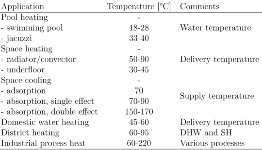
represen-tative ST collectors (compiled using data from: Hermann, 2011; Solar Keymark, 2017) and temperature ranges for several applications listed in Table 1.5: pool heating (PH); domestic hot water (DHW); space heating (SH); district heating (DH); space cooling (SC); industrial process heat (IPH). . . 16 1.6. Grid-connected forced circulation solar heating systems employing
tank charging methods reliant on: I) internal heat exchangers (top diagram); II) external heat exchangers and direct double ports (bot-tom diagram) . . . 19 1.7. Pressure-flow (left-hand side) and efficiency-flow (right-hand side)
curves for currently available pumps suitable for low-temperature ST systems . . . 22 1.8. Thermal efficiency curves (according to standards EN 12975-2:2006
Corp.). . . 27
2.1. Two diode equivalent circuit diagram for photovoltaic cells . . . 36
2.2. Block diagram for differential temperature static two-level hysteretic control (DTSTLHC). The pump state (Spump) is manipulated between
on and off states in accordance with the controller output (uc) while
the mass flow rate is allowed to deviate freely from the nominal value without corrective action. . . 54
2.3. Differential temperature static two-level hysteretic control function. . 55
2.4. Example of pump cycling in a low-temperature indirect DTSTLHC-operated ST system, using an internal heat exchanger as shown in Figure 1.6 (Spump, pump state; ∆T, temperature difference sensed;
Tcollector, fluid temperature at the collector outlet; Ttank, tank water
temperature at its bottom) . . . 56
2.5. Differential temperature static saturated hysteretic-proportional con-trol (DTSSHPC) characteristic curves with a: a) stepless linear ramp (thick straight line); b) discretised linear ramp (thick dashed line). . 60
2.6. Examples of DTSSHPC curves: left-hand side plot) convex, linear and concave functions defined by Swanson and Ollendorf (1979); right-hand side plot) linear function of the pump speed and resulting non-linear (convex) functions of the flow rate obtained through simulations for two different circulation pumps. . . 61
2.7. Simulated dynamic behaviour of a DTSSHPC-operated PV-T system during: I) a sunny day with low initial storage temperature, dur-ing which the nominal flow rate is reached; II) close-up of top left plot, highlighting oscillations during flow rate (step) transitions; III) a sunny day with moderate initial storage temperature, during which the nominal flow rate is not reached; IV) intermittent insolation day, during which the flow rate varies significantly and cycling is avoided until late in the day. These simulations relied on the model defined in Appendix D whose DTSSHPC implementation obeys a discretised linear m˙-∆T curve. . . 63
3 nodes; and DSC) reproduced from Schnieders (1997) to a collector inlet fluid temperature step from 20°C to 70°C. Note the new model’s convergence and imposed linearity issues for a small number of seg-ments on the left-hand side plot and, opposite it, the effect of the number of segments on the dead time. . . 85 3.3. Comparison between model responses (1, 3 and 30 segments) and
measured collector outlet fluid temperatures (second row plot) for significantly variable conditions (first row plot), according to data in Schnieders (1997). . . 86 3.4. Step responses of the proposed and HWB mean cell temperature
mod-els (second row plot) to mass flow rate, inlet temperature and irra-diance steps (first row plot). The models were parametrised accord-ing to the reference PV-T collector except with regard to: F′
UL,2=0
W/m2K2; ηpv,r=0%; and, Nseg=1 or 100. The reference irradiance
(GT,r) and specific mass flow rate (m˙c,r) used to normalise the input
variables were set to 1000 W/m2 and 0.013 Kg/m2s, respectively. . . . 88
3.5. Close-up of the irradiance step response of the proposed and HWB cell temperature models, previously shown in Figure 3.4. . . 89 3.6. Reference PV-T system single-day simulation results using the
pro-posed (“new”) and the Hottel-Whillier-Bliss (“HWB”) cell tempera-ture models: first row plot) normal sunny day (#4) with long col-lection period; second row plot) sunny day with low demand (#6), leading to hours of stagnation. . . 92 3.7. Reference PV-T system single-day simulation results using the
pro-posed (“new”) and the Hottel-Whillier-Bliss (“HWB”) cell tempera-ture models: first row) Sunny day with some clouds and no demand (#5), prompting some stagnation; second row) Cloudy day (#1), leading to limited pump operation. . . 93
4.1. Effect of measurement errors (ε) on controller behaviour and relation
to the actual (∆T) as opposed to measured temperature difference
(∆ˆT = ∆T +ε): left-hand side plot) overestimation errors (ε > 0) enable ∆T to go below ∆Tof f during operation, whereas
underesti-mation (ε <0) errors prove conservative; right-hand side plot) errors can contribute to and mitigate pump cycling. . . 102 4.2. Normalised PV generation-induced variation of∆Tof f,minand(∆Ton/∆Tof f)min
for cost-effective (Λpv,of f) and cycling-free (Λpv,on) operation,
respec-tively, according to the analytical Florschuetz model approach, for reference PV-T system-based parametric analyses of the normalised irradiance (GT/GT,r) and: first row) the overall collector heat loss
coefficient (UL); second row) the reference cell efficiency (ηpv,r) and
(right-hand side plot), according to the analytical method, for para-metric analyses on the irradiance (GT) and parasitic to auxiliary
en-ergy price ratio (Kpar,aux). . . 109
4.4. Normalised PV generation-induced variations of the minimum ∆Tof f
and ∆Ton setpoints for cost-effective (Λpv,of f; first row plot) and
cycling-free (Λpv,on; second row plot) operation of PV-T systems,
respectively, according to the numerical (N.A.; ∆Tof f = 2 K) and
Beckman et al. (B.A) approaches, for reference PV-T system-based parametric analyses of the irradiance level (GT) and the collector heat
loss coefficient temperature dependence (UL,2). . . 110
4.5. Minimum setpoint ratio (∆Ton/∆Tof f) for cycling-free operation and
its normalised variation (Λpv,on) due to PV generation, according to
the Beckman et al. (1994) (B.A.) and numerical (N.A.; ∆Tof f=2 K)
approaches, for parametric analyses on the irradiance level (GT) and
the reference cell efficiency (ηpv,r). . . 111
4.6. Effect of ∆Tof f on the minimum setpoint ratio (left-hand side plot)
for cycling-free operation of the reference PV-T system and its nor-malised variation (right-hand side plot) according to the numerical method and comparison with the Beckman et al. (1994) method, ver-sus the normalised irradiance (GT/GT,r). . . 112
5.1. Diagram for the active indirect grid-connected SDHW PV-T system reproduced in simulations for the purposes of the comparison between supply-loop differential temperature pump controls (DTSTLHC and DTSSHPC) . . . 117 5.2. Block diagram for the DTSSHPC variant studied: the pump speed is
the manipulated variable; the mass flow rate is the controlled variable.119 5.3. Example of throttling and pump speed adjustment . . . 120 5.4. Basic flowchart for the DTSTLHC model implemented . . . 122 5.5. Basic flowchart for the DTSSHPC model implemented . . . 123 5.6. Monthly horizontal irradiation (H) and average ambient temperature
(Ta,avg), by source location: Almería, Spain; Lisbon, Portugal (TMY
data); Freiburg, Germany (TMY data); De Bilt, Netherlands (TMY data). . . 124 5.7. Effect of ∆Ton and ∆Tof f setpoints on the fractional energy
sav-ings (fsav,aux) of SDHW PV-T systems using DTSTLHC, by nominal
specific mass flow rate (0.005, 0.01 and 0.02 Kg/m2s) and location (Almería and De Bilt). . . 130 5.8. Effect of ∆Ton and ∆Tof f setpoints on the electrical efficiency (ηpv,el)
( sav,aux) of SDHW PV-T systems using DTSSHPC (0 K≤∆ of f ≤2
K, ∆Ton = 3 K; 3 K≤ ∆Tof f ≤4 K, ∆Ton = 5 K; minimum specific
mass flow rate, 0.005 Kg/m2s), by nominal specific mass flow rate (0.01, 0.015 and 0.02 Kg/m2s) and location (Almería and De Bilt). . . 132 5.10. Effect of ∆Tsat and ∆Tof f setpoints on the electrical efficiency (ηpv,el)
of SDHW PV-T systems using DTSSHPC (0 K≤∆Tof f ≤2 K, ∆Ton
= 3 K; 3 K ≤∆Tof f ≤4 K, ∆Ton = 5 K; minimum specific mass flow
rate, 0.005 Kg/m2s), by nominal specific mass flow rate (0.01, 0.015 and 0.02 Kg/m2s) and location (Almería and De Bilt). . . 133 5.11. Range of normalised auxiliary energy savings differences (∆fsav,aux)
between equivalent DTSSHP- and DTSTLH-controlled SDHW PV-T systems utilising the same nominal specific mass flow rate, by system location. The symbols ◦ and denote the cases in which both
con-trols are configured to perform at their best and worst, respectively, whereas ◮ and ◭ point to the absolute optimum nominal flow rates
for DTSTLHC and DTSSHPC, also respectively. . . 135 5.12. Range of electrical energy efficiency differences (∆ηpv=ηpv,DT SSHP −
ηpv,DT ST LH) between equivalent DTSSHP- and DTSTLH-controlled
SDHW PV-T systems utilising the same nominal specific mass flow rate, by system location. The symbols ◦ and denote the cases
in which both controls are configured to perform at their best and worst, respectively, whereas ◮ and ◭ indicate the absolute optimum
nominal flow rates for DTSTLHC and DTSSHPC, respectively. . . 136 5.13. Monthly normalised auxiliary energy savings (above) and electrical
energy efficiency (below) differences between DTSSHPC- and DTSTLHC-operated SDHW PV-T systems using the same nominal flow rate (se-lected for the maximum annual ∆fsav,aux and ∆ηpv, respectively, to
highlight the variations) and otherwise configured to reach the max-imum auxiliary energy savings and electrical efficiency on an annual basis, respectively, for each location studied. . . 138 5.14. Pump running time (first row plot; ∆∆tpump = ∆tpump,DT SSHP C −
∆tpump,DT ST LHC) and normalised parasitic energy (second row plot;
∆fpar = [Epar,DT SSHP C−Epar,DT ST LHC]/Eaux,ref) differences between
DTSSHPC- and DTSTLHC-operated SDHW PV-T systems config-ured to reach the maximum auxiliary energy savings (denoted by the symbol:◦) and electrical energy efficiency (denoted by the symbol:⊳),
within the complete range of ∆∆tpump and ∆fpar (pipeline #1, cf.
Table D.1) results obtained. . . 140 5.15. Range of normalised primary energy savings differences (∆fP ES)
be-tween equivalent DTSSHPC- and DTSTLHC-operated SDHW PV-T systems utilising the same m˙nom/Ac. The narrow black band
repre-sents the ∆fP ES range for gas- and electricity-assisted PV-T systems
tems utilising the same m˙nom/Ac. The narrow black band represents
the ∆fF S range for gas- and electricity-assisted PV-T systems using
F S-optimised controls. . . 142 5.17. Normalised primary energy (∆fP ES) and financial (∆fF S) savings
dif-ferences between DTSSHPC- and DTSTLHC-operated SDHW PV-T systems configured for maximumP ES andF S, respectively (top row plots), and normalised PV yield (∆fpv), parasitic energy (∆fpar) and
auxiliary energy savings (∆fsav,aux) differences due toF S-optimisation
of each system (bottom row plots), by location and auxiliary heater (NG, natural gas-fired; E, electrical). . . 145 5.18. Normalised primary energy (∆fP ES) and financial (∆fF S) savings
dif-ferences between DTSSHPC- and DTSTLHC-operated SDHW PV-T systems configured for maximumP ES andF S, respectively (top row
plots), and normalised PV yield (∆fpv), parasitic energy (∆fpar) and
auxiliary energy savings (∆fsav,aux) differences due toF S-optimisation
of each system (bottom row plots; from left to right, respectively), assuming a fictitious 100% efficiency circulation pump, by location and auxiliary heater (NG, natural gas-fired; E, electrical). . . 147 5.19. Normalised financial savings (first row plot) and net present value
(second row plot, in e) differences between SDHW PV-T systems
using optimised DTSSHPC and DTSTLHC, as a function of the nor-malised natural gas price for each location (nornor-malised in relation to each location’s reference price) . . . 149
B.1. Collector efficiency factor as a function of the fluid temperature and specific mass flow rate, for the reference PV-T collector with PV gen-eration disabled (left-hand side plot), and collector efficiency factor range of variation due to the same factors while the PV-T collector is generating electricity, as a function of the normalised irradiance on the collector plane (right-hand side plot). . . 184
D.1. Pressure lift/drop versus flow rate curves (∆p-Q; above) and electri-cal power versus flow rate (Ppump,el-Q; below) curves, for the reference
high-efficiency variable-speed circulation pump and the various sys-tem pipelines (1-6). . . 191 D.2. Average monthly wind speed and mains water temperature. . . 192
E.1. Steady-state thermal efficiency curves using originally published data and those estimated using the method proposed, and comparison against the stagnation temperatures (Tstagnation) reported in Dupeyrat
1.1. Estimated global renewable energy potential by energy source and type of estimate, compiled from the following sources: Isaacs and Seymour (1973); Gustavson (1979); Barthel et al. (2000); Lako et al. (2003); Hoogwijk et al. (2004); Hermann (2006); Fridleifsson et al. (2008); Field et al. (2008); Trieb et al. (2009); Lu et al. (2009); Mork et al. (2010); Miller et al. (2011); de Castro et al. (2011, 2013); Gunn and Stock-Williams (2012); Schramski et al. (2015) . . . 8 1.2. Maximum PV module efficiencies measured under the global AM1.5
spectrum (1000 W/m2) and cell temperatures of 25°C (IEC 60904-3: 2008, ASTM G-173-03 global), discriminated by technology (adapted from Green et al. (2017)) . . . 9 1.3. Maximum power point (MPP) solar cell efficiency temperature
coef-ficients and energy bandgap (at 300 K), by PV technology (adapted from Affolter et al., 2005; Skoplaki and Palyvos, 2009; Emery, 2011) 11 1.4. Useful temperature range, concentration ratio and tracking
require-ments of relevant solar collector technologies (adapted from Kalo-girou, 2009) . . . 15 1.5. Design temperatures for selected ST-compatible low (<100°C) and
medium (<250°C) temperature applications (compiled from: Eicker, 2003, 2009; Kalogirou, 2003; Kaltschmitt et al., 2007; Weiss et al., 2003; GES, 2010; Lauterbach et al., 2012; Chow et al., 2012; Duffie and Beckman, 2013; Davis, 2015) . . . 18
3.1. Summary of mean plate temperature errors between the proposed (“new”) and HWB model responses (∆Tpv = Tpv,new −Tpv,HW B) to
the mass flow rate (m˙c), collector inlet fluid temperature (Tc,in) and
irradiance (GT) steps defined in Figure 3.4. The models were set up
after the reference PV-T system, except concerning the number of segments (100 segments) and where noted. . . 89 3.2. Summary of the comparison between the HWB (“HWB”) and the
proposed multi-segment (“new”) mean cell temperature models from single-day and annual simulations of the reference PV-T system using Almería, Spain climate data (HT, global irradiation on the collector
plane; ∆tpump, cumulative pump running time; ∆Tpv = Tpv,new −
single-day and annual simulations of the reference PV-T system using Almería, Spain climate data (HT, global irradiation on the collector
plane; ∆tpump, cumulative pump running time; ∆Tpv = Tpv,new −
Tpv,HW B; ∆ηpv =ηpv,new−ηpv,HW B) . . . 91
4.1. Parameter values for the reference PV-T system simulated . . . 106
5.1. Reference primary energy factors and energy prices for each location . 128 5.2. Highest normalised auxiliary energy savings (fsav,aux) obtained for
SDHW PV-T systems using DTSSHPC and DTSTLHC and the cor-responding nominal specific mass flow rate (m˙nom/Ac), for each
loca-tion considered. . . 142 5.3. Normalised financial savings (∆fF S) and net present value (NPV)
dif-ference incurred by opting for SDHW PV-T system using DTSSHPC instead of DTSTLHC, assuming reference energy prices, 0.25% dis-count rate, and fixed annual payments over a ten year period (NG stands for natural gas-fired backup heater, and E stands for electrical backup heater). . . 148
D.1. Parameter values used to configure the hydraulic submodel (the poly-nomial returns W when the independent variable is in Kg/s). . . 190 D.2. Parameter values used to configure the PV-T collector, thermal
Abbreviations
AC Alternating current
AM Air Mass
a-Si Amorphous silicon
a-Si:H Hydrogenated amorphous silicon
CCS Carbon Capture and Storage
CdTe Cadmium Telluride
CEN European Committee for Standardization
CIS/CIGS Copper indium (gallium) selenide
CPC Compound parabolic concentrator/collector
CSP Concentrated Solar Power
CTC Cylindrical trough collector
DC Direct current
DH District heating
DHW Domestic hot water
DNI Direct normal irradiance
DTSSHPC Differential temperature static saturated hysteretic-proportional con-trol
DTSTLHC Differential temperature static two-level hysteretic control
EC European Commission
EEI Energy Efficiency Index
FPC Flat-plate collector
FS Financial savings, e
GHG Greenhouse Gas
HDI Human Development Index
HFC Heliostat field collector
HWB Hottel-Whillier-Bliss (model)
IAM Incidence angle modifier
ICC Integral cycle control
IC Incremental conductance
IEA International Energy Agency
IEA-PVPS IEA’s Photovoltaic Power Systems Programme
IEA-SHC IEA’s Solar Heating and Cooling Programme
IEC International Electrotechnical Commission
IPH Industrial process heat
ISO International Organization for Standardization
LEC Low-emissivity coating
LFR Linear Fresnel reflector
mc-Si Monocrystalline silicon
MPP Maximum power point
MTOE Million Tonnes of Oil Equivalent
nc-Si Nanocrystalline silicon
NOCT Nominal operating cell temperature
NPV Net present value, e
pc-Si Polycrystalline silicon
PDR Parabolic dish reflector
PES Primary energy savings, kWh
PH Pool heating
PID Proportional-Integral-Derivative
PPA Power Purchase Agreement
PTC Parabolic trough collector
PV Photovoltaic
PV-T Photovoltaic-thermal
PWM Pulse width modulation
QDTM Quasi-dynamic test method
RPS Renewable Portfolio Standard
RTD Resistance temperature detector
SC Space cooling
SDHW Solar domestic hot water
SH Space heating
STC Standard test conditions
ST Solar thermal
TES Thermal energy storage
TMY Typical meteorological year
UV Ultra-violet
VRE Variable renewable energy
Greek Symbols
α Absorptance
∆fpar Normalised parasitic energy consumption difference
∆fP ES Normalised primary energy savings difference
∆fpv Normalised PV yield difference
∆fF S Normalised financial savings difference
∆p Pressure difference, Pa
∆T Temperature difference, °C or K
∆t Sampling time, s
∆tdelay Minimum pump running time, s
ˆ
∆T Temperature difference sensed by the controller, °C or K
∆Tof f Differential temperature controller turn-off setpoint, °C or K
∆Ton Differential temperature controller turn-on setpoint, °C or K
∆Tsat Differential temperature controller saturation setpoint, °C or K
∆Tsky Effective sky temperature difference, °C or K
∆x Segment length, m
ǫ Heat exchanger effectiveness
η Efficiency
η0 Zero-reduced temperature thermal efficiency (QDTM)
γpv Photovoltaic cell solar radiation coefficient
Λpv,of f Normalised PV conversion-induced variation of the minimum ∆Tof f
setpoint for cost-effective operation of PV-T systems
Λpv,on Normalised PV conversion-induced variation of the minimum ∆Ton
setpoint for stable operation of PV-T systems
ω Angular speed, rad/s
ρ Volumetric mass density, kg/m3
(τ α) Transmittance-absorptance product
τ Transmittance
θ Incidence angle relative to the collector plane normal, rad
ε Temperature measurement error, K or °C
Roman Symbols
A Area, m2
b0 Beam radiation incidence angle modifier coefficient
c1 Zero-reduced temperature heat loss coefficient for negligible wind
conditions (QDTM), W·m-2·K-1
c13 Zero-reduced temperature heat loss coefficient (QDTM), W·m-2·K-1
c2 Temperature dependence of the heat loss coefficient (QDTM), W·m-2·K-2
c3 Wind dependence of the heat loss coefficient (QDTM), J·m-3·K-1
c4 Sky temperature dependence of the heat loss coefficient (QDTM)
c5 Specific collector thermal capacity (QDTM), J·m-2·K-1
CA Specific collector thermal capacity, J·m-2·K-1
Cb Bond conductance, W·m-1·K-1
CE Bandgap energy temperature coefficient, °C-1
Cp Specific heat, J·kg-1·K-1
Ct,he Natural convection heat transfer coefficient for the storage tank heat
exchanger
D External diameter, m
d Internal diameter, m
E Energy, kWh
Eg Bandgap energy, eV
EL Longwave thermal irradiance (QDTM), W/m2
fp Primary energy factor
FR Collector heat removal factor
F′
R Collector heat exchanger factor
fsav,aux Fractional (end use) energy savings
G Irradiance, W/m2
g0 Zero-order coefficient (dynamic model fluid temperature equation),
W/m2
g1 First-order coefficient (dynamic model fluid temperature equation),
W·m-2·K-1
g2 Second-order coefficient (dynamic model fluid temperature equation),
W·m-2·K-2
g3 Specific thermal capacity (dynamic model fluid temperature
equa-tion), J·m-2·K-1
g4 Initial condition (dynamic model fluid temperature equation), °C
g5 Composite coefficient (dynamic model fluid temperature equation),
W·m-2·K-1
GT,on Minimum irradiance for useful heat collection, W/m2
Gz Graetz number
h Heat transfer coefficient, W·m-2·K-1
h0 Zero-order coefficient (dynamic model cell temperature equation),
W/m2
h1 First-order coefficient (dynamic model cell temperature equation),
W·m-2·K-1
h2 Second-order coefficient (dynamic model cell temperature equation),
W·m-2·K-2
H Horizontal irradiation, kWh/m2
HT Irradiation on the collector plane, kWh/m2
i Segment index
Io Dark saturation current due to recombination, A
Io,1 Dark saturation current due to recombination in quasi-neutral
re-gions, A
Io,2 Dark saturation current due to recombination in the depletion region,
A
j Sample index
K Incidence angle modifier
k Thermal conductivity, W·m-1·K-1
kB Boltzmann constant, J/K
(kδ) Thermal conductivity-thickness product, W/K
KI Photovoltaic cell current temperature coefficient, A/°C
Kp Pipeline coefficient, W·Kg-3·s3
Kpar,aux Parasitic to auxiliary energy price ratio
Kpv,el PV to general-purpose electricity price ratio
KV Photovoltaic cell voltage temperature coefficient, V/°C
L Length, m
m HWB model auxiliary variable, m
˙
m Mass flow rate, Kg/s
N Quantity
n Ideality factor
n1 Ideality factor corresponding toIo,1
n2 Ideality factor corresponding toIo,2
nt,he Natural convection heat transfer exponent for the storage tank heat
exchanger
N u Nusselt number
o3 Third-order pump power polynomial coefficient, W·Kg-3·s3
P Power, W
p Energy price, e/kWh
P r Prandtl number
˙
Q Heat flow rate, W
Q Volumetric flow rate, m3/s
q Electron charge, C
R Electrical resistance, Ω
Ra Rayleigh number
Re Reynolds number
S Solar radiation per unit area absorbed at the absorber plate, W/m2
Spump Pump state
T Temperature, °C or K
t Time, s
TR Reduced temperature, K·m2·W-1
Troom Room temperature, °C
uc Differential temperature controller control signal
Uf,p Thermal conductance between the absorber and the collector fluid,
W·m-2·K-1
UL Overall collector heat loss coefficient, W·m-2·K-1
UL,1 Zero-reduced temperature heat loss coefficient for negligible wind
conditions, W·m-2·K-1
UL,2 Temperature dependence of the heat loss coefficient, W·m-2·K-2
Usky Sky temperature dependence of the heat loss coefficient, W·m-2·K-1
uW Wind speed, m/s
V Voltage, V
Vload Daily load water volume, m3
Vt Tank volume, m3
W Riser tube spacing, m
x Position, m
Subscripts
a Ambient
aux Auxiliary
avg Time average
b Beam irradiance
c Collector
d Diffuse irradiance
ef f Effective
el Electrical, electricity
ext External
f Fluid
he Heat exchanger
in Inlet
ins Insulation
int Internal
m Spatial mean
max Maximum
min Minimum
out Outlet
p Absorber plate
gas Natural gas
par Parasitic energy
bos Balance of system
ph Light-generated
pipe Insulated pipe segment
pump Circulation pump(s)
pv Photovoltaic cell(s)
r Reference
riser Riser tube
s Series
sc Short-circuit
seg Segment
sh Shunt
stag Stagnation
step DTSSHP controller ramp step
T Tilted collector plane
t Thermal storage tank
th Thermal
u Utility
w Thermal storage tank wall
Miscellaneous
X∗
Reference value for variable X fed to controller ˆ
X Measured value of X quantity
f
1.1. Motivation
Technologies capable of supplying heat and electricity sustainably are set to be-come increasingly important in the context of climate change, depletion of fossil-fuel reserves and energy deprivation among humans. Many technologies are already ca-pable of doing so, directly or indirectly, yet solar thermal (ST) collectors and photo-voltaic (PV) panels are mature and can be successfully deployed in most of Earth’s regions and in a decentralised fashion. Similarly, hybrid photovoltaic-thermal (PV-T) collectors – which combine both technologies into a single design – can supply heat and electricity simultaneously while retaining a global and decentralised appeal. Despite the apparent abundance of renewable energy resources, particularly solar energy, and the proliferation of renewable technologies, there is growing doubt about the potential of such technologies to supply Mankind’s current and projected energy needs sustainably without major changes to the way human societies are organised. While by no means a panacea to such problems, PV-T technology has the advantage of potentially enabling a higher energy yield than separate side-by-side ST collectors and PV panels of equal combined area and effectively increase the useful energy density to maximise land use efficiency. At the same time, PV-T technology has not lived up to its potential, despite an already long maturation period, since some reliability issues still need to be addressed if it is to reach maturity.
The research efforts undertaken and summarised in this document concern knowl-edge gaps about the performance of solar domestic hot water (SDHW) PV-T systems with regard to the use of commonly available pump controllers. The following sub-sections lay out in greater detail the research activities conducted and the problems they seek to address, and prepare the reader to apprehend their significance and their potential application within the current context.
1.2. Context
1.2.1. Human development and sustainability
Development Index (HDI) for each country and the respective electricity consump-tion or other key energy consumpconsump-tion-based indicators (Pasternak, 2000; Martinez and Ebenhack, 2008; UNDP, 2011; Arto et al., 2016). However, more than 1 billion people worldwide – predominantly in Latin America, the Caribbean, Sub-Saharan Africa and South Asia – still lacked access to electricity in 2012, arguably the most versatile way to facilitate energy access today (Smil, 2004; UNDP, 2015).
On the other hand, the history of human development has been marred by, among other aspects, pollution, health hazards, loss of biodiversity and climate change, at least since the start of the Industrial Revolution (Crutzen and Stoermer, 2000; IEA, 2015b). Among these, climate change manifested through global average temper-ature increases, rising sea levels, retreating glaciers, permafrost thawing, among other trends, has arguably the most far-reaching implications and has been linked to anthropogenic emission of greenhouse gases (GHGs), particularly carbon dioxide (CO2) (Hansen et al., 2008; Montzka et al., 2011). Furthermore, the responsibility
for the bulk of cumulative GHGs emissions lies with developed countries and in recent years very high HDI countries – many of which are also among the highest cumulative GHG emitters – still emitted far more CO2 per capita than low, medium
and high HDI countries combined (UNDP, 2011; WRI, 2015; IEA, 2015a).
Several activities lead to GHG emissions but none more so than energy-related ser-vices, predominantly due to the combustion of fossil-fuels (IEA, 2015a; WRI, 2015). Despite its current role in human societies, the continued consumption of fossil fuels is bound to deplete reserves created over several hundred millions of years within a few decades or centuries at current production levels, while leading to catastrophic social, economic and environmental consequences in the process (Crutzen and Stoer-mer, 2000; IEA, 2013). In particular, climate scientists predict that the atmospheric concentration of CO2 should be, at most, 350 parts per million (ppm) to safely
prevent major changes to the Earth’s climate and species via global average tem-peratures 1.7°C below pre-industrial levels (Hansen et al., 2008). However, by 2016 the global average temperature had reached 0.99°C above pre-industrial levels and CO2 concentration levels reached 406 ppm in 2017, as seen Figure 1.1, increasing at
an average rate of 2 ppm/year over the past decade, which projections indicate will continue being the trend unless action is taken (Hansen et al., 2008; Dlugokencky and Tans, 2017; NASA/GISS, 2017; IEA, 2015b,a). As such, the prevailing model for human development needs to be quickly revised.
In this respect, the Paris Agreement entered into force1 in 2016 and commits 197
signatory countries to ensure the global average temperature remains “well below 2°C above pre-industrial levels” while pursuing efforts to “limit the temperature increase to 1.5°C” (UNFCCC, 2015). Notable for containing provisions to finance its implementation in developing countries by at least 100 billion USD per year – roughly 0.14% of gross world product in 2015 – the agreement has nevertheless
1
been criticised for encompassing private investment and financial instruments re-quiring repayment, such as loans with interest, in this financing goal (Orenstein, 2015; Buxton, 2016; OECD, 2015; World Bank, 2016). Several other criticisms have been levelled at the agreement including the exemption of international flights and shipping from GHG emissions’ calculations, the over-reliance on inconsistent and ex-perimental “negative emissions” technologies based on carbon capture and storage (CCS), the lack of enforceable mechanisms and the reliance on voluntary nationally determined pledges, revisable every 5 years (Milman, 2015a,b; Burt, 2015; Reyes, 2015). Regardless of intentions, the pledges for 2030 submitted up until late 2015 are projected to be insufficient to prevent global temperatures from exceeding 2°C above pre-industrial levels (IEA, 2015d; Peters et al., 2015; Rogelj et al., 2016). If confirmed, greater global political commitment is necessary for the agreement to conform with its purported aims and prevent “dangerous” climate change, namely by setting more ambitious targets and/or amending the agreement.
In addition to the absence of stronger international commitments on climate change mitigation, several challenges stand in the way of a timely transition towards sustainable human societies. In essence, these challenges concern the ability to sup-ply the current and projected global energy needs, according to the prevailing supsup-ply reliability standards, with the existing renewable energy potential, its geographical distribution, the existing technologies, the limited raw materials and respective re-cycling processes, all in a cost-effective, environmentally sound and politically viable way. The uncertainty about the feasibility of such a bold and quick transformation has been fuelled by recent publications. For instance, recent studies reported that wind, solar and biofuel power densities may be significantly lower than previously estimated (de Castro et al., 2011, 2013, 2014; Jacobson and Archer, 2012; Adams and Keith, 2013; Moriarty and Honnery, 2016; García-Olivares, 2016). Moreover, promising technologies such as concentrated solar power (CSP) plants, PV panels and wind turbines are reported to have higher raw material requirements per unit generation than conventional technologies, which may pose supply problems due to limited reserves and competition with other uses if these technologies are to be scaled up to meet current consumption levels (Vidal et al., 2013; de Castro et al., 2013; Hertwich et al., 2015; Jeffries, 2015). Thus, improvements in mining, recycling and energy efficiency are desirable and likely necessary to smooth the transition towards sustainability, as is the determination of the most efficient technologies in terms of land use and other relevant criteria such as energy return on energy investment (Vidal et al., 2013; de Castro et al., 2014; García-Olivares, 2016).
1.2.2. Energy outlook
addi-tion to this alarming scenario, the share of renewable energy sources2 in the global
primary energy demand is projected to increase from about 14% in 2013 to ap-proximately 15%, 19% or 30% in 2040 for increasingly optimistic projections, the most optimistic of which (“450 Scenario”) is only consistent with a 50% chance of limiting global average temperature increases to 2°C relative to pre-industrial lev-els (IEA, 2015d). Although inadequate to respond to the climate change challenge from an engineering standpoint, which prizes conservative design thresholds to en-sure an outcome, the projected increase will be felt in electricity generation, heat use (except traditional biomass, which is expected to decline) and transport, whose shares of renewables in 2013 corresponded to 22%, 10% and 3%, respectively, and are expected to reach between 27-53%, 14-22% and 5-18% in 2040.
Despite these projections, the currently limited contribution of renewables for transport contrasts with the double-digit shares for heat use and electricity gener-ation. Concretely, renewable electricity is still primarily provided by hydroelectric power plants (74% in 2013, down from 85% in 2008) and reached 16% of global electricity supply in 2013, whereas solar, wind and geothermal power accounted for less than 6%, despite notable capacity increases for wind and PV over the past decade – although behind hydropower, even in this regard (IEA, 2010, 2015d). Sim-ilarly, the vast majority (over 95%) of renewable heat is provided using bioenergy (including traditional biomass), accounting for around 25% of global heat in 2011, while ST and geothermal accounted for less than 1% of global heat and predomi-nantly within the buildings sector (Eisentraut and Brown, 2014; IEA, 2015d). Thus, modern renewable technologies for heat and electricity – although outpacing those for transport – are yet to make a significant impact on the global energy supply and among renewable technologies themselves, despite great strides in recent years. Nonetheless, according to IEA projections, renewable heat technologies other than traditional biomass are set to deliver between 14% and 22% of the final demand for heat in 2040 while non-hydro renewable technologies are poised to deliver more than half of renewable electricity generation, the majority of which from variable renewable energy (VRE) sources such as the sun and the wind (IEA, 2015d).
1.2.2.1. Renewable electricity
While part of the increase in renewable electricity generation projected for this century can be accommodated without major changes to existing power grids, the integration of the projected high shares of VRE technologies raises questions about the feasibility, cost-effectiveness and sustainability of maintaining the level of sup-ply reliability currently afforded by predominantly unsustainable yet dispatchable technologies (Steinke et al., 2013; Moriarty and Honnery, 2016; IEA, 2008, 2011,
2
2014). In essence, the fluctuating power output of VRE technologies may suddenly drop to a point that disrupts the supply of electricity – and increasingly so at higher penetrations of VREs such as in a 100% renewables scenario – unless compensated by dispatchable backup power generation and sufficient storage capacity, which cur-rent renewable technologies can’t provide to the extent that non-renewables can. Among the dispatchable renewables, hydropower and CSP plants are compatible with gravitational and thermal energy storage, respectively, but their deployment (as well as that of geothermal power plants) is geographically sensitive due to terrain and insolation, respectively, while the global potential for the expansion of installed capacity is limited for all including biomass power plants – arguably the only dis-patchable renewable technology not overly encumbered by geographical constraints (Field et al., 2008; WBGU, 2009; Steinke et al., 2013; Lako et al., 2003; Hamududu and Killingtveit, 2012; Fridleifsson et al., 2008).
So far, the countries with the highest shares of VREs (5-10%) in the respective energy mixes have not faced significant VRE grid integration challenges, which are only projected for shares above 25% (IEA, 2014). A recent example of the ability to handle current VRE power shortages occurred during the solar eclipse of March 20th 2015, which obscured the North Atlantic, Europe and North Africa for less than three hours. Estimates pointed to a maximum solar power reduction of close to 38% (34 GW) of the estimated installed capacity (90 GW) in the event of clear skies over Europe but the actual reduction only reached 19% and was handled by relying on alternative sources and demand reduction from the industrial sector (ENTSOE, 2015; Eckert, 2015). Future events, not limited to predictable and sporadic eclipses, are expected assume a greater importance as the share of VREs increases and in this sense the successful grid integration of VREs has been predicted to require enhanced energy storage capabilities, improved forecasting, better information and control of resources and loads, improved power system demand response, additional flexible capacity power systems and improved transmission networks (IEA, 2008, 2010, 2011, 2014; Steinke et al., 2013; Huber et al., 2014; Schaber et al., 2012).
1.2.2.2. Renewable heat
regions (POSHIP, 2001; ECOHEATCOOL, 2006). Concurrently, ST heat is a po-tential option in the high temperature segment for industries located in high direct normal irradiance (DNI) sunbelts, but whose deployment is set to remain limited until 2050, according to the IEA 2°C scenario (Eisentraut and Brown, 2014; IEA, 2015d). Nevertheless, industries will face increasing pressure to adjust to local re-newable resources or relocate, in order to meet sustainability goals (Moriarty and Honnery, 2016). As such, the need to adjust industrial processes to existing renew-able technologies, and vice-versa, to increase renewrenew-able heat use has been recognised and research efforts have been directed for this purpose (Frank et al., 2012).
1.2.2.3. Solar energy potential
Solar energy is presently an abundant renewable energy source on Earth and is expected to remain so for the foreseeable future3 (Eicker, 2003; Schröder and Smith,
2008; IEA, 2010). Each year, about 5,500,000 EJ of incoming solar energy reaches the Earth’s upper atmosphere, about 30% of which is reflected back to outer space, leaving a net contribution to the Earth’s energy balance of roughly 3,850,000 EJ (Gustavson, 1979; Smil, 1999, 2003, 2008). In comparison, the global primary energy supply for the year 2013 amounted to 567 EJ, or roughly 0.01% of the annual net solar contribution (IEA, 2015c). At the same time, only part of the incoming solar radiation can be harnessed for stationary ground-level applications due to constraints such as geographical incidence, limited siting options, variable weather conditions and intermittency caused by syzygies and Earth’s rotation on its axis. The influence of these factors leads to estimated geographic potentials of solar energy at least two orders of magnitude lower than the net solar contribution, whereas additional technical, economic or sustainability considerations further reduce its potential by up to three additional orders of magnitude, as summarised in Table 1.1. As such, covering mankind’s current energy needs may not be possible only with direct solar energy but will likely require a diverse range of energy sources instead.
1.3. Review of selected solar energy technologies
The prospect of a limited role of solar energy in supplying mankind’s energy needs makes developing and selecting the most land use and energy efficient solar energy technologies increasingly important. Solar energy technologies include – but are not limited to – ST collectors, CSP plants and PV panels which supply heat for final use, electricity from solar heat and electricity from photoelectric conversion, respectively. Photovoltaic-thermal (PV-T) technology, the focus of this study, is a hybrid variant of ST and PV technology – two of the most deployed solar energy technologies – capable of supplying heat and electricity simultaneously. As such, the states of PV and ST technologies are benchmarks for PV-T technology and
3
Table 1.1.: Estimated global renewable energy potential by energy source and type of estimate, compiled from the following sources: Isaacs and Seymour (1973); Gustavson (1979); Barthel et al. (2000); Lako et al. (2003); Hoogwijk et al. (2004); Hermann (2006); Fridleifsson et al. (2008); Field et al. (2008); Trieb et al. (2009); Lu et al. (2009); Mork et al. (2010); Miller et al. (2011); de Castro et al. (2011, 2013); Gunn and Stock-Williams (2012); Schramski et al. (2015)
Source Geographical Technical Economic/Sustainable Unit Hydropower 130-158 50-52 25-29 EJ/year Geothermal 1,010-600,000 8-140 - EJ/year Wind 568-6,000 32-640 32-221 EJ/year Solar 1,575-689,203 - - EJ/year Solar (CSP) - 10,605 - EJ/year Solar (PV) - 726-15,463 65-130 EJ/year Biomass 2,000-2,900 276-446 27-270 EJ/year
Tidal 79-85 - - EJ/year
Wave 65-117 3 - EJ/year
relevant for a correct assessment of its merits and shortcomings, particularly for those unfamiliar with all of the above technologies. The following sections briefly review all three technologies, with emphasis on terrestrial, non-concentrating, low-temperature applications, particularly SDHW, where applicable.
1.3.1. Photovoltaics
1.3.1.1. Overview
Photovoltaic cells and modules are semiconductors optimised to generate elec-tricity when exposed to solar radiation. Several semiconductor technologies can be used for PV conversion, each with its specific spectral sensitivity to electromag-netic radiation, which can be combined in tandem (multi-junction cell) to obtain a broader spectral response and higher efficiency, practical considerations notwith-standing. The respective theoretical efficiency limits were determined to be 34% for single junction cells at 25°C and under one sun (1000 W/m2, AM1.5 spectrum) whereas for tandem solar cells with an infinite number of junctions the limits were determined to be 68% and 87% for one and multiple suns (i.e., concentrated light4),
respectively (Shockley and Queisser, 1961; de Vos, 1980; Goswami, 2015).
As of 2017, maximum PV conversion efficiencies for non-concentrating technolo-gies using single- and multi-junction cells are in the 9-29% and 13-39% ranges, respectively, and up to 46% for concentrator cells. However, maximum efficiencies for a given technology at a point in time are generally obtained using small
labo-4
Table 1.2.: Maximum PV module efficiencies measured under the global AM1.5 spectrum (1000 W/m2) and cell temperatures of 25°C (IEC 60904-3: 2008, ASTM G-173-03 global), discriminated by technology (adapted from Green et al. (2017))
Photovoltaic Technology Efficiency [%] FF [%] Area [m2] Date mc-Si (monocrystalline) 24.4 ± 0.5 80.1 1.32 09/2016 pc-Si (polycrystalline) 19.9 ± 0.4 79.5 1.51 10/2016 GaAs (thin film) 24.8 ± 0.5 84.7 0.09 11/2016 CdTe (thin film) 18.6 ± 0.6 74.2 0.70 04/2015 CIGS (Cd free) 19.2 ± 0.5 73.7 841 01/2017 CIGS (large) 15.7 ± 0.5 72.5 0.08 11/2010 a-Si/nc-Si (tandem) 12.3 ± 0.3 69.9 1.43 09/2014 Organic 8.7 ±0.3 70.4 0.08 05/2014 InGaP/GaAs/InGas (tandem) 31.2 ± 1.2 83.6 0.10 02/2016
ratory cells rather than mass-produced non-concentrator multi-cell modules, which represent the bulk of installed capacity. Accordingly, peak efficiencies for technolo-gies using single- and multi-junction non-concentrator modules are in the 9-24% and 13-31% ranges, respectively, as summarised in Table 1.2 (Green et al., 2017).
Solar cells do not inherently function at their peak electrical conversion efficiency but are rather conditioned by the incident radiation’s intensity and spectral dis-tribution, local weather and load matching. Naturally, incident solar radiation is essential for the conversion to occur and higher irradiance (GT) levels enable a higher
electrical power output, as illustrated on the right hand side of Figure 1.2. Con-currently, the absorption of solar radiation also heats up the cells and along with
Figure 1.3.: Simulated effect of cell temperature on the current, voltage and ef-ficiency curves of a crystalline-silicon photovoltaic module (under 1000 W/m2, AM1.5 spectrum; using the model and parameters from Villalva et al., 2009)
other heat transfer mechanisms, such as longwave radiative heat transfer, natural and wind-based forced convective heat losses and thermal bridges, sets the oper-ating cell temperature, whose influence on cell efficiency is generally negative as exemplified on the right hand side of Figure 1.3 (Skoplaki and Palyvos, 2009).
On the other hand, the load characteristics also influence the performance of solar cells. The effects of cell voltage (V), current (I), temperature (Tpv) and irradiance
(G) are exemplified in the characteristic current-voltage (I-V) curves of Figures
1.2-1.3, which reveal a maximum power point (MPP) for each individual I-V curve, electrical output power levels rising with increasing irradiance levels as well as pos-itive and negative temperature coefficients for the short-circuit current (Isc) and
open-circuit voltage (Voc), respectively. The combined effect of open-circuit voltage
and short-circuit current variations as temperatures increase adversely affects the efficiency (or power output) of most solar cells at the MPP, given how the former’s temperature coefficient is higher and negative. Thus, the MPP efficiency of most PV cells exhibits a negative temperature coefficient (βpv), often modelled as linear
Table 1.3.: Maximum power point (MPP) solar cell efficiency temperature coeffi-cients and energy bandgap (at 300 K), by PV technology (adapted from Affolter et al., 2005; Skoplaki and Palyvos, 2009; Emery, 2011)
Photovoltaic MPP efficiency temperature Energy Bandgap Technology coefficient [%/°C] [eV] 0.53 eV GaInAs -0.76 to -0.60 0.53 0.75 eV GaInAs -0.72 to -0.50 0.75 CIGS (CuInxGa1-xSe2) -0.65 to -0.24 1.04-1.68
pc-Si (polycrystalline) -0.50 to -0.32 1.12 mc-Si (monocrystalline) -0.52 to -0.29 1.12
InP -0.41 to -0.16 1.27
GaInP/GaAs -0.21 to -0.19 1.85/1.42
GaAs -0.27 to -0.19 1.42
CdTe -0.41 to -0.12 1.44
a-Si -0.26 to -0.05 1.6-1.8
a-Si (tandem) -0.23 to -0.00 1.6-1.8/1.1-1.7 1.7 eV AlGaAs -0.17 to -0.10 1.7
given the approximately fixed relative proximities of the MPP voltage and current to the open-circuit voltage and the short-circuit current, respectively, which tend to hold even as the irradiance or cell temperatures change – see Figure 1.3 (Luque and Hegedus, 2011). Nevertheless, direct methods tend to perform best and are generally independent of the module type (Hohm and Ropp, 2000, 2003; de Brito et al., 2013; Bendib et al., 2015; Rezk and Eltamaly, 2015).
1.3.1.2. Applications
The electricity produced by PV modules, either at the MPP or not, can be stored, used locally or fed to local utility grids efficiently through the use of power converters. Grid-connected PV systems, which make up a majority of existing systems, typically inject electricity into local AC grids using MPP-tracking capable inverters or sepa-rate converters for each conversion stage (IEA-PVPS, 2016c). Similarly, autonomous PV systems rely on one or more power converters to charge electrochemical batter-ies and/or supply loads while performing MPP tracking or not. Moreover, MPP tracking in autonomous systems is possible as long as the loads and/or batteries can accommodate the respective power output, whereas grid-connected systems are gen-erally prevented from supplying electricity during blackouts as a safeguard against the islanding phenomenon5 (Bollen and Hassan, 2011; Karimi et al., 2016). Known
autonomous applications include powering orbital satellites, spacecraft for inner So-lar System exploration, water pumps, weather stations, communication equipment
5