Francisco Antero Cardoso Marques
Licenciado em Ciências de
Engenharia Electrotécnica e de Computadores
A Flexible Navigation System for Autonomous
Robots Operating in
Heterogeneous Environments
Dissertação para obtenção do Grau de Mestre em
Engenharia Electrotécnica e de Computadores
Orientador: José António Barata de Oliveira,
Professor Auxiliar, FCT-UNL
Copyright
A Flexible Navigation System for Autonomous Robots Operating in
Heterogeneous Environments
A Faculdade de Ciências e Tecnologia e a Universidade Nova de Lisboa têm o direito, perpétuo e sem limites geográficos, de arquivar e publicar esta dissertação através de exemplares impressos reproduzidos em papel ou de forma digital, ou por qualguer outro meio conhecido ou que venha a ser inventado, e de a divulgar através de repositórios científicos e de admitir a sua cópia e distribuição com objectivos educacionais ou de investigação, não comerciais, desde que seja dado crédito ao autor e editor.
Acknowledgements
I would like to express my gratitude to my dissertation supervisor Prof. José Barata for his inva-luable support and for giving me the outstanding opportunity to work on the robotics domain. Also like to thank co-supervisor Prof. Pedro Santana for the motivation, knowledge and support and also for opening me the world of robotics. Also the fun and extremely noisy research team members An-dré Lourenço, Carlos Sousa, Eduardo Pinto, Gonçalo Cândido, Giovanni di Orio, Pedro Gomes and Ricardo Mendonça.
IntRoSys, S.A for giving me the opportunity for working in the Introbot project, especially Magno Guedes and Pedro Deusdado from helping me on the innumerous times I needed to test the robot.
André Lourenço, Pedro Pinto and Rui Borrego for the countless hours passed studying in the last couple of years.
Abstract
This dissertation presents a flexible navigation system for autonomous robot operating in hetero-geneous environments. In the proposed system, flexibility occurs at several levels of the navigation system. At the lowest level, proper locomotion modes are selected according to the local context, which includes handling dynamic footprints when computing traversability costs. This flexibility en-sures that the kinematic and morphological constraints of the robot are adequately considered when navigating in demanding environments. At the highest level, proper motion planning strategies are selected according to the global context, namely, the expected topology of the environment. This flexibility allows the robot to trade-off, in a context-aware way, accuracy of the planned motions and computational cost. As a result, the complexity of the planner matches the complexity of the envi-ronment, which is key to enable a proper management of computational and energetic resources. Following a pragmatic strategy, the robot obtains its global context from off-line generated maps, which are becoming widely available. To validate this idea, a tool for semantic labelling of satellite im-agery was developed. Online, the robot obtains its global context extracting the semantic label (e.g., urban environment) and distribution of expected obstacles associated to its current global position. The proposed system leverages on the well-known Robotics Operating System (ROS) framework for the implementation of the navigation system underpinnings. For extensive validation purposes, a physics-based 3D simulator was used. Moreover, the system was validated over 1 Km long experi-ments on a physical four-wheeled robot. The results obtained show the ability of the system to ensure safe navigation in heterogeneous environments. This is a result of the ability of the system to exploit context awareness to reconfigure itself when facing transitions among topologically different environ-ment regions. The added level of robustness introduced with the proposed system is expected to foster the application of autonomous robots in socially relevant domains.
Resumo
Esta dissertação apresenta um sistema flexível de navegação destinado ao controlo de robots autónomos em ambientes heterogéneos. No sistema proposto, a flexibilidade abrange diversos ní-veis. Num primeiro nível, o modo de locomoção correcto é escolhido de acordo com o contexto local, compreendendo o cálculo do custo de cada trajetória onde se inclui o seu footprint dinâmico. Num nível mais elevado, as estratégias de planeamento são seleccionadas de acordo com o contexto global, nomeadamente a topologia esperada do ambiente. Assim, seguindo uma estratégia prag-mática, o robot extrai o contexto global de mapas gerados offline e, posteriormente, extrai a etiqueta semântica e a distribuição dos obstáculos associados à sua posição global actual. A validação do sistema foi feita, num primeiro momento, através de um simulador 3D de ambientes físicos, e depois, através de diversas experiências com um robot físico onde foi percorrido aproximadamente 1 km de distância. Os resultados obtidos mostram que o sistema permite uma navegação autónoma segura em ambientes heterogéneos, o que se deve sobretudo à sua competência para se reconfigurar pe-rante transições entre regiões topologicamente diferentes. É esperado que este nível adicional de robustez possibilite a aplicação de robots autónomos em domínios socialmente relevantes.
Contents
List of Figures xiii
List of Tables xvii
1 Introduction 1
1.1 Dissertation Outline . . . 2
2 Related Work 3 2.1 Robot Motion and Path Planning . . . 3
2.1.1 Local Planning . . . 3
2.1.2 Global Planning Methods . . . 6
2.2 Robot Localization and Mapping . . . 8
2.2.1 Kalman Filtering . . . 9
2.2.2 Markov Localization . . . 9
2.2.3 Monte Carlo Localization . . . 10
2.2.4 Mapping . . . 11
2.2.5 Simultaneous Localization and Mapping . . . 11
2.3 Semantic Information . . . 13
3 Real and Simulated Robot 15 3.1 The Introbot Robotic Platform . . . 15
3.2 Introbot’s simulated Model . . . 18
3.3 Introbot’s Software Architecture . . . 21
4 Flexible Navigation System 25 4.1 Semantic Labels and Environment Types . . . 27
4.4 Global Path Planning . . . 30
4.5 Local Trajectory generation . . . 31
4.6 Localization . . . 35
5 Experimental Results 37 5.1 Experimental Setup . . . 37
5.2 Results . . . 37
5.2.1 Narrow Spaces . . . 38
5.2.2 Open Spaces . . . 46
5.2.3 Transition . . . 49
5.3 Discussion . . . 51
6 Conclusions and Future Work 61 6.1 Conclusions . . . 61
6.2 Future Work . . . 62
List of Figures
2.1 The dynamic window approach . . . 4
2.2 Trajectory roll out approach . . . 5
2.3 Markov localization . . . 10
3.1 Robot sensor package . . . 16
3.2 Introbot locomotion modes . . . 16
3.3 Robot laser scanner range coverage diagram . . . 18
3.4 Overview of robot model architecture . . . 19
3.5 Robot model transform tree . . . 20
3.6 Simulated Worlds . . . 20
3.7 Simulated mathematics department offline map . . . 21
3.8 Software Architecture . . . 22
4.1 Flexible navigation system architecture overview . . . 26
4.2 Snapshot of design tool . . . 28
4.3 Semantic mode waypoint to goal calculation method . . . 29
4.4 Same goal with path generated from different planners . . . 31
4.5 Dynamic footprint advantages in trajectory creation . . . 32
4.6 Robot’s possible trajectories . . . 33
4.7 First situation of plan heading calculation . . . 33
4.8 Second situation of plan heading calculation . . . 34
4.9 Third situation of plan heading calculation . . . 34
4.10 Failures cases of plan heading calculation . . . 35
4.11 EKF input sources . . . 36
5.3 Semantic map used in the indoor narrow space experiment . . . 39
5.4 Trajectory of robot during indoor field test . . . 39
5.5 Robot dealing with first turn . . . 40
5.6 Robot dealing with u shaped turn . . . 40
5.7 Snapshot of the route to the third goal . . . 41
5.8 Robot stuck . . . 41
5.9 False positives . . . 42
5.10 Avoidance of a dynamic object . . . 43
5.11 Outdoor location . . . 44
5.12 Semantic map used in the outdoor narrow space experiment . . . 44
5.13 Robot’s narrow-space path . . . 45
5.14 Snapshot of the route to the initial goal . . . 46
5.15 Snapshot of the robot moving alongside a pedestrian . . . 47
5.16 Example of bad localization . . . 47
5.17 High speed avoidance . . . 48
5.18 Robot near the third goal . . . 48
5.19 Path to the other side of the building . . . 49
5.20 Snapshots of events on the way to sixth goal . . . 50
5.21 Snapshot of the final goal run . . . 51
5.22 GPS location overview . . . 51
5.23 Semantic map used in the waypoint following experiment . . . 52
5.24 GPS route . . . 53
5.25 Snapshots of initial goals . . . 53
5.26 False positives caused by terrain roughness and vegetation . . . 54
5.27 Snapshots of the approach to steel fences area . . . 55
5.28 Snapshot of avoidance situation . . . 56
5.29 Semantic map used in the experiment . . . 56
5.30 Transition experiment route . . . 57
5.31 Semantic map used in the transition experiment . . . 57
5.32 Snapshot of GPS part of the run . . . 57
5.34 Snapshots of particle dispersion in the localization of the robot . . . 58
List of Tables
Chapter 1
Introduction
The motivation behind this dissertation is the development of a flexible navigation system for autonomous robots operating in heterogeneous environments.
Using this type of control system, field robots may perform diverse tasks such has surveillance, search and rescue, environmental monitoring, and forest preservation.
Autonomous robot navigation was always widely studied, (Brooks, 1986; Arkin, 1989; Elfes, 1989; Kuipers and Levitt, 1988), and has proven to be a complex and interesting subject. Complexity increases if robots are to navigate in unstructured and heterogeneous environments. Even though some field robots already have the capability to navigate in complex environments, may they be off-road (e.g., (Thrun et al., 2006; Crane et al., 2007; Miller et al., 2006; Behringer et al., 2005; Braid et al., 2006)) or urban (e.g., (Urmson et al., 2008; Montemerlo et al., 2008; Miller et al., 2008; Chen et al., 2008)), the ability to transition between them remains an open problem.
Furthermore, autonomous robots’ navigation systems developed to date cannot operate with the same level of performance in heterogeneous surroundings, as if they were built specifically to operate in one of them. One solution to the transition problem may be the use of topological maps (e.g., (Thrun, 1998)) to limit immense complexity of using more accurate metric maps when transitioning areas. Another solution is to use multiple-hierarchical semantic information (e.g., (Galindo et al., 2005)) to improve the system’s adeptness to the surrounding environment. Other is to use scene classification to identify the type of surroundings and adjust navigation accordingly (e.g., (Collier and Ramirez-Serrano, 2009)). Finally, the extraction of semantic from satellite imagery can be used produce cost maps and traversable calculation (e.g., (Silver et al., 2006)), thus, adapting to the terrain.
This dissertation approaches the problem differently by proposing a flexible control system ca-pable of exploiting local environment semantic information to adjust the navigation system to the surrounding’s context. This way the robot is able to navigate in urban environments, off-road envi-ronments, and indoors without human intervention. Moreover, the smooth transition between these environments is also ensured.
level, context is retrieved from offline labelled overhead satellite imagery. At the second level, context is extracted from the robot’s local perception sources.
The proposed system has flexibility at different levels to ease the adaptation and transition be-tween diverse environments. This new level of robustness provides the robot with the tools to adapt and chose proper strategies according to the context.
To validate the proposed system, field trials were conducted on New University of Lisbon campus, where a robot with four independently steered wheels navigated autonomously for approximately 1 km at 0.5 meters per second over an operating period of 30 minutes.
During these trials the robot never collided even when facing different dynamic objects. More-over, it was capable of reaching all of the navigational goals while transiting between heterogeneous environments.
Finally, regarding the main objective it was able to transition between open space and narrow space environments.
In sum, the results provided enough experimental data to show that the system is: (1) capable of providing autonomous robots with safe navigation behaviour; (2) capable of robustly handling GPS signal dropouts; (3) able to deal with noisy perceptual data causing obstacles false alarms; and (4) able of successfully exploit semantic information for smooth transitions between environments.
1.1
Dissertation Outline
This dissertation is composed as follows:
Chapter 2 reviews the state-of-the-art for mobile robot navigation.
Chapter 3 displays the Introbot robot platform, software architecture and simulator setup. Chapter 4 describes the proposed navigation system and its components.
Chapter 5 presents the experimental setup and the set of results obtained, their strength and weak-ness;
Chapter 6 aggregates a set of conclusions, main contributions of this dissertation, and further
Chapter 2
Related Work
The main objective of this chapter is to introduce the reader to the basic components, the whole multitude of methods and best practices that can be applied when building a mobile robot’s navigation control system.
Initially, robot motion and path planning methods are presented in Section 2.1, which is followed by an explanation concerning robot localization and mapping techniques (see Section 2.2), and finally the usefulness of semantic information (see Section 2.3) as more complex and robust behaviours are required.
It will be made clear how some methods are better suited for structured environments such as in-door navigation or urban facilities while others perform better navigating in unstructured and dynamic environments such as all-terrain or troublesome scenarios.
2.1
Robot Motion and Path Planning
One of the fundamental functions of a mobile robot’s navigation system is to safely avoid obsta-cles, and that is something that this first section aims to explain.
In subsection 2.1.1 obstacle avoidance and reactive techniques are addressed with special regard to their benefits and setbacks. Subsequently a description of global planning methods is exposed (see subsection 2.1.2), to bridge the most basic type of navigation constraints (e.g., obstacle avoid-ance) to the broader sense of the navigation’s ultimate goal.
2.1.1
Local Planning
the robot’s secure transition between its current position to a goal point in space. The goal can be either just a midway point of the whole path or simply a specific heading or even a final pose (position and heading). In the case of path following the local motion control increased granularity provides the means to correct global path errors, which would be unperceivable from the global planner coarser perspective. For the robot’s local planner to behave in a reasonable fashion, the trajectory generation procedure needs to take into account the dynamics of the robot. The solution to this problem is not a trivial one, in fact, its complexity hinders a system from performing adequately in a whole variety of situations. This subsection presents some of the most relevant robot motion methods, namely the Dynamic Window Approach (Fox et al., 1997) and The Trajectory Roll Out (Gerkey and Konolige, 2008).
Dynamic Window Approach
(a)
Figure 2.1:The dynamic window approach (a) The dynamic window approach where the black rectangle
rep-resents the window of possible velocity tuples (Fox et al., 1997)
In the Dynamic Window Approach (Fox et al., 1997) the main objective is to endow the mobile platform with appropriate reactive avoidance to handle the perilous situations the robot could find itself. The time factor is of crucial importance since it has to conciliate the dynamics of both the robot and the environment. This is attainable by taking into consideration the robot’s motion dynam-ics to effectively reduce the search space of motion control possibilities, effectively lightening the computational load.
2.1. Robot Motion and Path Planning
Trajectory Roll Out
(a)
Figure 2.2: Trajectory roll out approach (a) The controller generates trajectories by sampling feasible
veloci-ties and simulating their application over a short time horizon. Generated trajectories are purple, the chosen trajectory is yellow, the desired global path is cyan, and obstacles are red (Gerkey and Konolige, 2008)
The Trajectory Roll Out (Gerkey and Konolige, 2008) takes the opposite direction that of the Dynamic Window Approach. In this method the search is limited to the space of feasible controls in contrast to feasible trajectories, confining the search to seek a good instead of the optimal control. The control space is normally defined as two-dimensional pairs of linear and angular velocities (e.g., surface robot) in which the sampled region is narrowed by the above-mentioned search policy. The simulation then predicts with a discrete time approximation of the robot’s dynamics, this returns a path composed of 5 dimensional states. The trajectories simulated are then evaluated by a weighted cost (see Equation 2.1).
C(t) =αObs(t) +βGdist(t) +γP dist(t) +δ 1
x2(t) (2.1)
In which there are three components, Obs that is the sum of the grid cell costs of the trajectory; Gdist is the estimated shortest distance to the goal; Pdist that is the estimated shortest distance to the path;X that is the translational part of the velocity command;α β γare parameters to control the weight of each component.
tried first then selecting the best of the legal trajectories, next if none of the forward velocities is valid, the in place rotations are sampled and if those are not valid also, the robot finally tries to backup. This supervisory node is used to promote progress if that is deem possible. As in the Dynamic Window Approach the acceleration limits may difficult the parameterization.
2.1.2
Global Planning Methods
The Local Navigation based architectures are adequate when dealing only with basic navigational needs, nevertheless they lack a broader sense of awareness. Hence, cannot assure an optimal path when traveling from point A to point B. Additionally this limitation can also take the robot into un-foreseeable and troublesome situations, being thecul-de-sacone of the classical examples. Indeed
this known limitation in conjunction with the greater availability of computational power fostered the adoption of global path planners. Global planning is indeed a fundamental part of most mobile robot navigation systems. Some of the most relevant path planners are overviewed in the following sec-tions.
Dijkstra
Edsger Dijkstra developed the Dijkstra’s algorithm (Dijkstra, 1959) in the mid-1950, a graph search based algorithm capable of finding the shortest path between two vertices (Graph Geodesic). The objective is when supplied with a certain start and goal vertices to find the path with lowest cost connecting them.
To find the optimal path all the vertices are initially marked as unvisited by placing their distance to the goal as infinity. Subsequently, the initial node is set as the current position and tentative distances to neighbouring nodes (part of the unvisited set) are calculated saving the shortest distance to each of them. Then, after considering all neighbours in the vicinity the current node is set as visited and removed from the unvisited set. Afterwards, a verification occurs to find if the goal is marked as visited or if the smallest distance in all of the unvisited list comprising nodes is infinity, if any of the above conditions is valid the search comes to a halt. However, if this is not the case, the unvisited node with the shortest tentative distance is marked current and the algorithm goes on.
Even though it is capable of finding the shortest path between two points, the Dijkstra’s algo-rithm search is unfocused, with no hierarchy regarding its expansion. For this reason its inefficient compared with the subsequent algorithms.
A*
2.1. Robot Motion and Path Planning
node (g()) to an heuristic (h()) that estimates the distance from the current node to the goal (equation
2.2).
f(x) =g(x) +h(x) (2.2)
Normally an optimistic linear distance is used for the heuristic function so that its admissible, that means that it does not overestimate the distance to the goal. Starting in the initial node aopen set is
created organized in a priority queue, sorted by the lowest cost of the distance plus cost function. At each iteration the node with lowest cost is removed from the queue and the other nodes are updated and re-queued. This recursive behaviour is repeated until the goal node was the lower cost value of all the priority queue. Then, goal cost is only the path length, because at the goal the distance to goal is zero.
By focusing the search using heuristics the A * algorithm effectively diminishes the domain of search enabling it to cope with large search spaces, and so outperforming Dijsktra algorithm in that type of situations.
ARA*
The Anytime Repairing A* (Likhachev et al., 2003) algorithm is a response to real world problems than cannot be solved by traditional optimal planners. In conclusion anytime planners are the answer to situations where the response of the planner is more important than the optimality of the path. In some situations there is not an unlimited time frame to create an optimal path, so anytime planners arose to solve this issue. Providing a sub optimal answer in a short time and then continuously improving the solution is one way to solve the time frame demands.
One hypothesis to create a Anytime planner is to use A* search (Anytime A*) with inflated heuris-tics. To inflate the heuristics a parameterǫis multiplied with the normal heuristic function (always ǫ >1). This provides a bound on the desired sub-optimal path equal to theǫvalue. By continuously decreasingǫ, a range of sub-optimal solutions is created, where the length of the solution is no larger thanǫtimes the optimal path length.
Nonetheless, this approach searches start always from scratch, thus not capitalizing on previously gathered information, effectively wasting computational power. So in ARA*, A* is started with a largeǫ and run several times always lowering the value until an optimal path is returned, but at the same time each iteration uses previously search information making the algorithm faster than normal Anytime A*.
D* Lite
the search were always restarted. The D * lite algorithm (Koenig and Likhachev, 2002) also aims to reuse information gathered in previous searches and focusing the search by using heuristics methods as in A* (Hart et al., 1968).
The planner is designed to determine the shortest path between the vertex where the robot is located and the goal vertex by monitoring the vertex cost change whilst the robot is moving. Search direction is from goal to the robot position and the shortest path is travelled by minimizing the cost function and braking ties arbitrarily.
The reuse of previous search information is possible with the introduction of Right Hand Siderhs computation, that represents the value of a vertex parent plus the cost to travel to that vertex. The planner detects local inconsistencies by comparing this computation to the cost of that vertex, en-abling it to update graph information while moving. In a normal situation therhsand the node cost are equal and so locally consistent. Therefore, when the node cost is different from therhscomputation the cost changed dynamically. Inconsistency falls in two different types: under consistency where the node cost is lower than therhscomputation meaning that the vertex is now more expensive and the paths that pass through this node need to be recalculated; over consistency is when the node cost is greater than therhsmeaning that the path to this vertex is now less expensive and this information is used to manage the search open list.
When there are no inconsistencies the algorithm is the same as the A*. Nevertheless, when there are local inconsistencies those vertex are added to the open list. Subsequently, the algorithm is always checking for graph changes to add them to the open list refreshing key values when there is updated connection data and not only with new connections. This happens when the robot advances, heuristics decrease because the movement is towards the goal and so connections change and thus key values are recalculated.
2.2
Robot Localization and Mapping
In this section a brief overview of localization and mapping applied to mobile robotics is presented. Initially several localization methods are addressed followed by mapping techniques. Localization is an essential issue when working with mobile robots, the capability of estimating the robot’s position in an environment is paramount for an effective autonomous navigation. In other words the ability of the robot to know its position in a reliable way is essential for a large array of mobile robotics applications.
There are two categories of localization the major difference being the demand of prior knowledge of the initial robot’s position, while tracking techniques need this type of information global techniques do not require data concerning the initial localization. As a result the first approach is useless in case of a wrong initial estimate or if the robot becomes delocalized outside certain bounds. Whereas global techniques are capable of coping with no initial information about the robot’s position. This means that they are able to handle the kidnapped robot problem where a robot is carried to an
2.2. Robot Localization and Mapping
a brief overview of mapping techniques is provided in subsection 2.2.4, followed by the conjunction of localization and mapping a problem known as SLAM (Simultaneous Localization and Mapping) is explained in subsection 2.2.5.
2.2.1
Kalman Filtering
Kalman filtering (KF) is a case of probabilistic state estimation used in mobile robotics (Kalman et al., 1960). The Kalman filter contains two different models, the plant model and measurement model. In mobile robotics the plant model represents the relationship between motion controls and the robot position, where the measurement model is the data provided by the robot sensor package related to its current position. The KF uses a two-step predictor algorithm in a form of force feedback, first it projects the predicted state estimate and the error covariance from the earlier state obtaining thea priori estimates for the next state. The feedback occurs when a sensor measurement is
re-ceived, it corrects the predicted state estimate by using the measurement to generatea posteriori
state estimate. This cycle is repeated after each time step and measurement update.
The applicability of the traditional Kalman Filter to localization in mobile robotics is impaired by the its incapability of handling nonlinear systems, this is because mobile robots tend to be highly nonlinear. For that reason in mobile robotics variations of KF that can cope with nonlinear systems are normally used, like Extended Kalman Filter (EKF) (Jazwinski, 1970) or Unscented Kalman Filter (UKF) (Julier and Uhlmann, 2004). To handle with nonlinear systems the EKF linearizes all nonlinear transformations and replaces the Jacobian matrices for the linear transformations in the traditional Kalman Filter. This of course is only robust if the error propagation can be approximated by a linear function. However, the major drawback of using Kalman Filtering in mobile robotics is due to its uni-modal nature so it cannot localize the robot from scratch. Furthermore, it can quickly diverge if not properly initialized, in fact its incapable of recovering from this type of failures.
That said Kalman Filters are successfully used in mobile robotic applications (Leonard and Durrant-Whyte, 1991, 1992; Schiele and Crowley, 1994).
2.2.2
Markov Localization
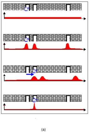
Another probabilistic method used for mobile robot localization is Markov Localization (Fox et al., 1998). By maintaining a probability distribution over the space comprised by all possible robot loca-tions, it weighs all possibilities and makes an mathematical assumption regarding the robot’s position.
the probability in all the remaining positions. The next step in the localization method is the handling of robot motion. After moving and by considering the noise induced by the uncertainty intrinsic to robot motion, the probability is smoothed lowering the certainty of the robot’s current location. Then, robot queries it sensors and updates the perception information, using this new data the probability of certain locations is raised. Leading to a new and more accurate belief. All of this steps are evident in Figure 2.3.
In essence Markov localization is a multi-modal discrete state space localization technique, which provides a robot with the capability of robustly locate itself in static environments that is has prior knowledge about. However, it is also possible to apply Markov Localization to dynamic environments, as it was showed by Fox’s work (Fox et al., 1999) were this was achieved by the introduction of filtering techniques .
(a)
Figure 2.3:Markov localization (a) The basic idea of markov localization: A mobile robot during localization (Fox et al., 1998) In the top image the robot’s position probability density (in red) is spread equally in all the positions. After the sensors of the robot detect that it is near a door, so the locations near a door have their probability raised. The robot moves (blue arrow) and the certainty of its position lowers. The sensor is queued and the robot is localized with a high probability.
2.2.3
Monte Carlo Localization
2.2. Robot Localization and Mapping
scratch. Nevertheless, Markov Localization is also global localization technique but at the expense of large amounts of memory and computational burden. Furthermore, Monte Carlo Localization is more accurate than Markov Localization if the grid cell size is fixed. To implement Monte Carlo Localization a particle filter is used, in the next paragraph the particle update process is described.
First the next generation of particles is created from the previous generation and by sampling the probabilistic motion odometry model as a proposal distribution. Then, the particles are weighted according to a importance sampling principle related to sensor measurements.
This importance weighting method is the likeability of each particle according with the sensor in-formation available. In other words the difference between the predicted measurement and the actual measurement. The next step is resampling, where particles are retrieved randomly but proportional to their importance weight. Making the particles with better probability more likely to live on, where the lower probability particles tend to disappear. The random nature of the resampling is an impor-tant part of the particle filter algorithm, because if only the particles with higher probabilities lived on there is a risk of finding only a local maximum. After this resampling all the particles have the same weight and the cycle returns to the first step. These approaches combine the advantages from the previous localization methods, are capable of multi-modal and globally localize the robot.
2.2.4
Mapping
In this subsection an outline of some mapping techniques is provided, with emphasis on topolog-ical mapping and merging topologtopolog-ical with metric maps. Typtopolog-ically, topologtopolog-ical maps are represented as graph states, in which nodes represent landmarks, places or regions and paths represent the trajectories that will take an autonomous agent from one region to another. In Remolina and Kuipers work (Remolina and Kuipers, 2004) an overview on how to merge sensory input, topological and local metric information, into a topological map is presented. Also Thrun (Thrun, 1998) stresses the efficiency of using topological representations when solving large scale planning opposed with the immense complexity of using more accurate metric maps with grid-base methods. Nevertheless, he also states that generating accurate and consistent topological maps is a difficult task, and so presents the hypothesis of generating topological maps on top of grid-based metric maps. This per-spective tries to combine the accuracy off metric maps and the efficiency of using topological maps to planning problems. A similar approach is also defended by Kuipers et al. (2004) the use local metrical information for the small-scale space and topological maps for the large-scale space. While Konolige et al. (2011) proposes a method to build topological map using a graph SLAM system, local navigation metric maps are also used. The major advantage of all the aforementioned methods is the faster global planning provided by the use of a topological graph in opposition of a full metric map, at the same time maintaining a safe navigation behaviour by using metric maps for local navigation.
2.2.5
Simultaneous Localization and Mapping
in some circumstances (Thrun et al., 2000). In other situations where the environment is unknown, for instance a search and rescue operation this is not possible. Creating a problem because the localization errors are now incorporated in to the creation of the map representation, limiting the operation of mobile robots in such situations.
The incorporation of localization errors in the creation of the map is a technique known as Simul-taneous Localization and Mapping (SLAM) and will be described in this subsection.
The ability to build maps is one of the essential capabilities of a mobile robot when faced with uncertain environments. However, it is a complex problem, it requires a conjunction of a robust localization and consistent mapping. This two premises normally are mutual dependent, to generate a trustworthy map a reliable location is needed and vice-versa. In essence uncertainty created by the robot motion when building a map forces the robot to also perform localization. Several solutions are available they can be based in Kalman Filter approaches (EKF-SLAM) or on probabilistic methods (particle filters) (Montemerlo et al., 2002, 2003; Grisetti et al., 2007), there are also differences in map representation while some use grids others use topological maps. All approaches deal with the same basic problem, they need to estimate online both the trajectory of the robot and the location of landmarks withouta priori information. In this subsection a brief and simplified explanation of how
these approaches function will be presented.
The solution using EKF suffers from the same problems described in the aforementioned 2.2.1 Kalman Filtering localization subsection, but it also profits from the its strong points. In this type of implementation the robot motion depicted by an EKF and landmark observations are used for the measurement updates. The EKF-SLAM updates all the landmarks and covariance matrixes at each observation measurement, entailing a great computational burden. Nevertheless, some optimized variations showed that they can deal efficiently with a large number of landmarks. Another important issue in this type of implementation is the strong dependency of sound association between observations and landmarks, if this association becomes incorrect the EKF-SLAM algorithm fails.
To solve some of the limitations of the EKF solution, some implementations shifted to particle fil-ters, namely RAO-Blackwellized particle filters (Montemerlo et al., 2002, 2003; Grisetti et al., 2007). The particle filter is used to estimate the posterior of the map using the robot’s motion, the estimation provided by sensor observations and odometry measurements. In a Rao-Blackwellized filter the com-putation is done first by estimating the trajectory of the robot and then generating a map associated with that motion. Amongst the most studied models, the FastSLAM model (Montemerlo et al., 2002, 2003) represents a robot trajectory hypothesis with a particle and each map landmark is indepen-dent. This means that each map (particle) is composed from independent landmarks represented by a Gaussian distribution. Every observation of a landmark is treated as an EKF measurement update of that trajectory, which is represented in by single particle.
2.3. Semantic Information
a meaningful area by using a scanmatcher algorithm starting from an initial pose guess, sampling is then done with points centred around the region of interest return by the scanmatcher. This leads to a new particle pose, based on this improved proposal distribution, the importance weights are updated, and each map (particle) is refreshed according to the pose and observation, followed by resampling. This focusing of the search produced by the use of scan-matching effectively diminishes number of particles needed, and so reduces computational load, in addition resampling is also optimized to reduce the risk of particle depletion.
SLAM adds the capability of operating in unknown terrain. This of course is only interesting in certain situations and environments. Mainly because of the computational burden associated, in other words whena prioriknowledge is easily obtainable the advantages of SLAM are overpowered
by the need to save computational power. That said SLAM is one of the most important mobile robotics achievements.
2.3
Semantic Information
By extracting semantic from the environment the realm of tasks performed by mobile robots can grow in complexity and robustness. In this subsection two different uses of semantic data extraction are described. First, scene classification used to exchange navigation modes between indoor and outdoor scenarios. Second, semantic data is extracted from overhead imagery to improve global navigation.
Scene Classification
Collier and Ramirez-Serrano (2009) uses image classification to determine the operating mode of the robot. By extracting features from image perception information and training a classifier using supervised learning, the system is able to adapt to two different types of environments, indoors and outdoors. A autonomous robot normally is designed to operate in only one type of environment and could fail when faced with different surroundings. Scene classification adds the capability of categorizing the surrounding context, enabling the robot to use this information in the decision making process.
Initially images from sensor streams are analysed and certain features are extracted: color His-tograms, RGB, HSV, LUV, color spaces; orientation histograms computed form horizontal and vertical Sobel Images; color moments from HSV and LUV; curvature histograms computed form vertical and horizontal Sobel images. These features are then classified by using either artificial neural networks or support vector machines, the resulting classification is then used for the informed exchange of the robot’s mapping system. In outdoors the robot uses a 2.5D map by integrating range data from stereo pair and pose estimates from GPS and IMU into a grid-based map. In the indoor mode an EKF-SLAM algorithm is used based on a 2D map representation.
semantic data improves the scope and performance of the navigation system.
Long Range Navigation Using Overhead Data
Chapter 3
Real and Simulated Robot
In this chapter the autonomous vehicle used in the implementation of this thesis is presented. First, the real Introbot is presented in Section 3.1, where a brief description of the mechanical struc-ture, hardware and perception is provided. Then, the contribution made by creating a simulation platform is presented in Section 3.2 based on the Gazebo simulator and is composed by a robot sim-ulation model and a couple of simsim-ulation worlds. Finally, in Section 3.3 the Robot Operating System (ROS) based software architecture is presented, with a brief overview of the contributions.
3.1
The Introbot Robotic Platform
The Introbot is a versatile outdoor robotic platform with quasi-omnidirectional motion for real world applications such as surveillance, agriculture, environmental monitoring and other related domains. It was develop in a joint effort by SME Portuguese company IntRoSys, S.A.1, LabMAg of the University
of Lisbon2and Uninova CTS3in the context of the QREN project Introsys Robot4.
1IntRoSys, S.A.❤tt♣✿✴✴❤tt♣✿✴✴✇✇✇✳✐♥tr♦s②s✳❡✉
2LabMAg of the University of Lisbon❤tt♣✿✴✴❧❛❜♠❛❣✳❞✐✳❢❝✳✉❧✳♣t
(a)
Figure 3.1:Robot sensor package (a) Overview of perception sensor package
(a) (b)
(c) (d)
3.1. The Introbot Robotic Platform
The introbot was designed to operate in diverse kinds of terrains and situations allowing fully and semi-autonomous control intended to work on outdoor real world applications.
The operational versatility of the Introbot is possible because of a robust modular hardware archi-tecture mainly composed by off-the-shelf components. The sensor package is composed by multi-plicity of perceptional devices that include a 2-D laser scanner (see Figure 3.3), a ring of ultrasonic sensors, a stereoscopic vision sensor, and a set of monocular cameras (see Figure 3.1). Addition-ally, also an inertial measurement unit (IMU) with a built-in global positioning system (GPS) device is available to enlarge the realm of perception sources, in this case mostly suited for localization and navigation. Processing is assured by a 2.4 ghz 4 gigas ram Pentium(R) Core 2 duo CPU T4300 2.10GHz with4Gb of RAM, running a32-bit Linux distribution Ubuntu 10.10 (Maverick Meerkat) in-dustrial board for basic functions, and to perform more complicated tasks there also the possibility of adding additional processing.
To detect problems that could result in a lower operational readiness the robot possesses self-monitoring and diagnosis capabilities. This is accomplished by integrating several internal sensors responsible for gathering temperature readings, voltage and current drawn, and controlling the health of the battery.
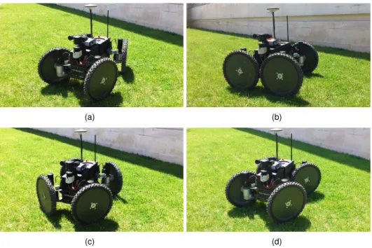
Another important asset included in the Introbot design is the no-slip quasi-omnidirectional lo-comotion structure. Based on a 4x4 independent wheeled system, it can provide up to five types of movement (see Figure 3.2). This choice has multiple advantages, it reduces mechanical stress, energy consumption, and for localization and navigation purposes it avoids large odometry errors. This versatility is possible by coupling directly each motor to their corresponding wheel through a gear instead of chains or belts. Furthermore this reduces energy loss and more importantly the num-ber of failure points. All of this in conjunction with the aggregated power of all motors, exceeding 1 kW maximum, allows the robot to navigate at up to1.5ms−1and overcome up to45degrees incline slopes.
Another issue often neglected in current robotic platforms is the ease of their transportation and storage. It has a medium sized footprint (800mm×1500mm×700mm) and weight, 100 Kg. Also,
each wheel supports hand locking and manual clutch, and the longitudinal passive axis can also be locked in the central position. All of the above characteristics ease the manual transportation of the Introbot.
(a)
Figure 3.3: Robot laser scanner range coverage diagram (a) Top view of laser scanner range coverage where
blue arrow represents the robot’s orientation and the sensing area of the laser scanner is represented in green.
3.2
Introbot’s simulated Model
The use of simulation was indispensable in the development of the system presented in this dis-sertation. Despite the clear differences to real world situations and restricted complexity, it permitted to surpass the limited amount of time and resources for testing using the Introbot. The parallel de-velopment of hardware components meant these opportunities were scare and so the capability of testing new software developments in a simulated environment facilitated the development cycle. Therefore, a simulation setup was created based on the ROS framework that provided both software and hardware in the loop capabilities. The simulation was based on the Gazebo simulator5for ROS.
A robot model was created using the Unified Robot Description as well as simulated sensors and actuators. Additionally for a better simulation performance and fidelity there were also developed software simulations of the Introbot sensor and actuators interface (see Figure 3.4). In this section will be presented the URDF model creation, the sensor actuator controllers and interface software simulation as well as simulation worlds.
3.2. Introbot’s simulated Model
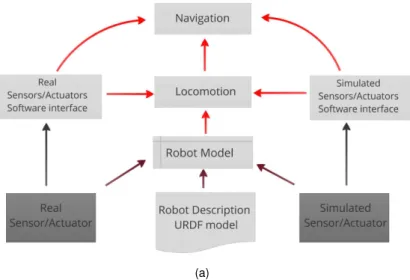
(a)
Figure 3.4: Overview of robot model architecture (a) Robot model architecture, by adding a simulated layer of sensor and actuators software interface, the same robot model and Unified Robot Description Format (URDF) description can be used for the simulated and real robot. In this figure the dark grey/red arrows represent low level sensor streams and the transforms tree messages of sensor/actuator respectively. The red arrows are higher level messages (ROS topics) exchanged by nodes or groups of nodes (stacks). The robot model is loaded into the ROS master and becomes available to all the nodes in the system such as the locomotion node or navigation stack.
To fully integrate a robot within the ROS framework a model representation has to be created, for this purpose ROS relies on a description language based on Extensible Markup Language (XML) called URDF. The language depicts models in a tree structure and can only be used on robots complaint with this type of representation. Nevertheless, the modelling process is not limited only to the description of mechanical properties, it also must contain additional information about sensor placements and part dimensions. In the next paragraph a summary of the inner workings of the URDF language is presented to improve the reader’s understanding of its limitations and possibilities.
The URDF language is based on two major type of components, links and joints, a link is basically a part that has both visual and collision representations, whilst a joint simply unites two different links. A joint has a parent and a child link and it can be of flexible or inflexible nature. In inflexible joints only the origin in relation to the two links is defined, flexible joints however have another set of characteristics mainly concerning the kind of displacement they allow. There are five types of flexible joints: the revolute joint that rotates a certain angle around a defined axis; the continuous joint that is a special type of revolute joint that can rotate indefinitely; the prismatic joint that moves along an axis, not around it; the planar joint that has translational movement around two axes; and, finally the floating joint that is basically and unconstrained joint.
plug-ins so a new one was developed using geographic_ info6 ROS package. By exploiting a not fully
implemented parameter in the description of a simulated Gazebo world, it was possible to create a new reliable GPS simulation. The parameter in question was used in conjunction with the provided ground truth positioning and the assumption that theX axis of the reference frame points north and theY points east. Then, basically the ground truth position was added to the centre position to get a (Universal Transverse Mercator) UTM geo-referenced position. The UTM position was then con-verted to longitude latitude, additionally a Gaussian error was also added to get a more reliable GPS simulation. Actuators were also modelled using tools provided by ROS, a PID controller simulator was implemented for each wheel both for traction and steering. The controllers tuning process was carried out by using the Ziegler Nichols method (Ziegler and Nichols, 1942) to adjust the motor re-sponse to better mimic that of the real robot. Despite all of the similarities to the actual Introbot, it
(a)
Figure 3.5: Robot model transform tree (a) The robot model transform tree is the structure that maintains the
relationship between coordinate frames in a tree structure, each ellipse represents a frame.
was also necessary to simulate the intermediate layer (controller nodes) that connected the low level PID controllers to the higher level kinematic control. This step added the possibility to transition from the simulated model to the real robot in a seamless and effortless way.
(a) (b)
Figure 3.6:Simulated Worlds (a) Snapshot of Indoor world. (b) Snapshot of Outdoor world both red and green
represent3Dmodels of buildings .
3.3. Introbot’s Software Architecture
Finally to complete the simulation setup it was necessary to turn to the simulation of the environ-ments the robot was designed to travel. This meant that two kind of settings were needed, first an indoor world and second an outdoor large scale ambiance. For the indoor simulation there was no need for modification and so the stock office world that comes with gazebo was used (see Figure 3.6(a)). This world represents the inside of an office building, several office furniture models and other objects were inserted during the simulation tests including tables, chairs etc.
(a)
Figure 3.7:Simulated mathematics department offline map (a) Image of generated map where grey stands for
unknown space, white represents free space and black are lethal obstacles.
For the remaining tests another world was designed to simulate the grounds of the Faculty of Science and Technology of New university of Lisbon (Figure 3.6(b)). To achieve this effect first a satellite image with approximately 500 for 250 m of the selected area was obtained, this image was then overlaid in Gazebo on top of the simulation ground plane. To further increase realism existing 3D models of Faculty buildings were added, as well as some trees and diverse objects. This world was essential to test the transition between environments by enabling the realization of offline maps (see Figure 3.7) of certain key areas, that then were used for both single semantic zone navigation as well as the semantic zone transitions.
The ability to simulate this type of environments proved to be crucial in finding problem areas, moreover, it aided the testing new software developments and parameters. In sum the simulation capability of this system provided tools invaluable to both the basic functions (motion, kinematic control, sensor streams) as well as higher level capacities ( navigation, perception algorithms).
3.3
Introbot’s Software Architecture
The ROS framework was created to deliver appropriate tools to manage the complexity of soft-ware needed to operate a robot, For example the large service robots have multiple processing units and sensors and high bandwidth demands because of the large amount of data exchanged between them. To resolve these issues the ROS framework already provides standard operating system ser-vices such as hardware abstraction, low-level device control, message-passing between processes and package management. Joining all of these functionalities the framework provides tools for dis-tributed computing development, capable of running applications across multiple computers. The basic architecture is based on a peer-to-peer graph like topology, in which nodes process data asyn-chronously at the same time that they can receive, post or multiplex messages, which can carry any type of previously defined data such as sensor control, actuator state and planning messages.
(a)
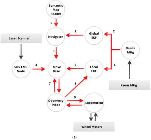
Figure 3.8: Software Architecture (a) Overview of the software architecture, each number represents a mes-sage stream between nodes. The red arrows represent mesmes-sage passing between nodes, the grey arrows represent sensor/actuator data acquired by the node using the sensor/actuator API. (0) std_ msgs/UInt16 Semantic Zone, sensor_ msgs/NavSatFix (1) geometry_ msgs/PoseWithCovarianceStamped (2) sensor_ msgs/NavSatFix (3) move_ base_ msgs/MoveBaseActionGoal (4) sensor_ msgs/LaserScan (5) geometry_ msgs/PoseWithCovarianceStamped (6) sensor_ msgs/Imu (7) geometry_ msgs/Twist, nav_ msgs/Odometry (8) nav_ msgs/Odometry (9) sensor_ msgs/JointState, sensor_ msgs/JointState
3.3. Introbot’s Software Architecture
• Low level control and sensor interfaces, in this group are included all the sensor/actuators low level interfaces.
• Locomotion control, this group is responsible for the locomotion of the robots composed by two nodes the kinematics/odometry node and Locomotion node. The odometry node receives a message that represents the desired linear an angular velocity (geometry_ msgs/Twist) and
transforms it into kinematic valid wheel velocities and steering angles (sensor_ msgs/JointState),
it also receives wheel encoder data stream (sensor_ msgs/JointState) and then publishes an
estimated robot pose in form of a odometry message (nav_ msgs/Odometry) . The
locomo-tion node receives wheel velocities and steering angles and sends this desired values to the motor controllers and also collects wheel encoder data in form of a ROS message (sensor_ msgs/JointState).
• Perception is composed by the Sick LMS Node and Xsens Mtig Node. The Sick LMS Node pub-lishes the planar laser data stream in a ROS complaint message (sensor_ msgs/LaserScan).
The Xsens Mtig Node publish two different types of messages and 3D orientation message (sensor_ msgs/IMU) and a GPS message (sensor_ msgs/NavSatFix)that are both used for
localization.
• Navigation is composed of a group of nodes in charge of semantic label extraction, large scale navigation, path planning and obstacle avoidance behaviours (Navigator, Global EKF, Local EKF, Move Base). By receiving and fusing sensory information (sensor_ msgs/LaserScan,
(sensor msgs/IMU), position and velocity estimates (nav_ msgs/Odometry) and desired goal
poses (move_ base_ msgs/MoveBaseActionGoal), provided respectively by the perception
nodes, odometry and Navigator, it publishes a path to the desired goal as well as the next angular and linear velocities (geometry_ msgs/Twist) to the locomotion control node. This is
Chapter 4
Flexible Navigation System
The major contribution of this thesis is the navigation module developed. To better cater the needs of the navigating in complex and heterogeneous settings, severe modifications were needed to the traditional architecture of an autonomous robot navigation system. This chapter presents an overview of the modifications and their interactions (see Figure 4.1) followed by an analysis of each component in greater detail.
As it is evident by the statements above any navigation architecture contains a large amount of data being exchanged between its components and also from and to the hardware of the platform. This is one of the reasons for using the ROS navigation stack as a starting point, because its frame-work already provides support for message passing and synchronization. Also the ROS navigation stack already has a functional basic architecture (Marder-Eppstein et al., 2010) that contains several of the traditional navigation components, such as:
• Occupancy grid;
• Global Planner;
• Local Planner;
• Recovery behaviours.
Despite the good results of most of the basic navigation architectures evidenced in some type of situations. The majority of basic architectures also have some limitations that restrict the scope of possible tasks. The most meaningful limitations to the type of system this thesis tries to create are enumerated below:
• Inability of dealing with large-scale environments;
• No capability of adjusting online to the environment;
• Limit to one online global planner;
(a)
Figure 4.1: Flexible navigation system architecture overview (a) The navigation system joins many different
nodes and stacks, this figure shows an overview of the different nodes and interactions inside the navigation system. Each red arrow represents an interaction utilizing ROS topics, each bracket contains a category of nodes, the red arrows are ROS topics, the black arrows are low level sensor/actuator messages, the dark red arrows represent parameters.
• Only designed for differential drive and holonomic wheeled robots only;
• Developed for a square robot, so its performance will be best on robots that are nearly square or circular.
Is this type of pitfalls that the new developed navigation module tries to respond and resolve, enabling the robotic platform with the capability to navigate in complex and diverse of environments. A new set of modules, plugins and additional tools where designed to address these problems.
4.1. Semantic Labels and Environment Types
the global planning, to enhance the planning proficiency a supervisory module can choose online between different global planners(subsection 4.4). Finally the modified local planner is capable of dealing with quasi-omnidirectional robots with dynamic footprints(subsection 4.5).
4.1
Semantic Labels and Environment Types
To enrich the situational awareness of the autonomous mobile platform there was a need of higher level information, in other words the limited scope of the perception tools available to the robot do not provide enough information, both in quality as well as in quantity to empower the robot to travel in a multitude of environments.
The approach taken in this thesis is to furnisha priori information by semantic labelling overhead
satellite imagery. In this iteration of the stack only two different labels were used, one represents an open space while the other symbolizes a narrow space area. When talking about open spaces the label encompasses diverse environments with the common feature being as the name entails large open spaces, normally natural or rural ambiances. Narrow space areas can also represent a large range of settings, with the prevalent characteristics being the large amount of obstacles as well as the absence of GPS signal, these a normally urban settings both indoor or outdoor.
Using this information the system can by using its flexible nature adapt to the requirements and challenges of the aforementioned types of surroundings. The nature of these challenges as well as the steps the navigation stack takes to respond to them will become clear in the following subsections.
4.2
Control Center and Path Design Tool
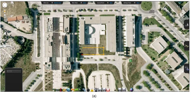
For the control center and path design the choice was a Web User-Interface based on Google Maps API1, designed to serve as a control center to monitor the position and infer high-level path and
behaviour planning to the robot system of the Introbot platform. The Google API was a first stepping stone to the application construction, as it already had built in waypoint drawing and positioning over a map in a well adopted user-friendly environment. Above a layer of multiple features intended to smooth the path design, the application gathers a special group of traits:
• User register (login) system;
• Management of user paths files in accordance to known GPS standards (GPX2,KLM3) verified with distributed xml schemas;
• Asynchronous Communication with the robots via Dropbox4synchronization;
• Live tracking of the current position (or path) of the robots on the map. 1Google Maps API❤tt♣s✿✴✴❞❡✈❡❧♦♣❡rs✳❣♦♦❣❧❡✳❝♦♠✴♠❛♣s✴
2GPX❤tt♣✿✴✴✇✇✇✳t♦♣♦❣r❛❢✐①✳❝♦♠✴❣♣①✳❛s♣
(a)
Figure 4.2:Snapshot of path design tool (a) Snapshot of path creation using path design tool, orange represents a designed path, green circle is the path origin, red circle is the path end.
The application was constructed as a Java Server Page assembling Javascript (Google maps API and JQuery Library5) to both implement the path design over the Google Maps and ease the control
panels in and out of the application, and AJAX to request any user-related feature, such as the logging in or the file submission. The unreliable nature of the communication with both outdoor robots over remote areas led to the decision of introducing also an asynchronous mean of communication to complement the ROS message service, a file like synchronization over the internet through Dropbox, had to be the solution, given its simplicity and practicality. The auto-planner option provided renders a simple and intuitive approach to path planning. An image of the region of interest defined by the two selected points is retrieved from Google Static Maps API and a path planner based on Field D* Algorithm (Ferguson and Stentz, 2007) provides a list of waypoints that are then marked back on the map as new path or subpath.
4.3
Waypoint Navigation
Large scale navigation is one of the necessities of autonomous robots. Thus, in the proposed system a node takes on the role of supervising the navigation stack enabling it to perform large scale navigation. This subsection is dedicated to explain the inner workings of this node.
Initially the node receives a plan created in the control center, containing an array of geo-referenced waypoints that form a path to be followed by the robot. Given such plan the waypoints are transformed
4.3. Waypoint Navigation
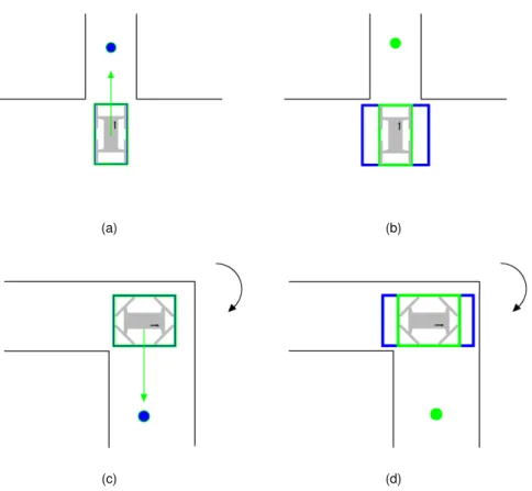
(a) (b)
Figure 4.3:Semantic mode waypoint to goal calculation method (a) Narrow space , first the distance from robot to map center (red square) is calculated (blue arrows), then distance from goal to map center also computed (orange arrows) and finally goal (green circle) can be sent to robot global navigation path planner (green arrows). (b) Open space, distance from robot to goal is calculated (blue arrows) and goal (green circle) is sent to robot global navigation path planner (green arrows).
to navigation goals, however, the goal transformation process is semantic zone dependent. In other words the waypoint to goal process has different steps according to robot’s semantic location.
However, both transformations share a similar step, the geo-referenced positions are transformed from longitude and latitude to UTM coordinates. UTM coordinates represents the world in two-dimensional Cartesian coordinates, this is achieved by dividing the world in sixty zones and using a secant transverse Mercator projection in each one. Therefore, with the robot position and way-point/goal position represented in UTM coordinates and in conjunction with the robot’s heading its possible simply calculate the Euclidean distance between them, this distance is then fed to the robot navigation.
Whilst this suffices in the case of the Open Space where there are only this two positions and the reference frame is robot centric. In the Narrow Space semantic zone the goal has to be map referenced. To solve this issue the map centre position is also geo-referenced therefore possible to transform to UTM coordinates. Thus allowing the use of simple Euclidian distance, to transform a waypoint/goal from a geo-referenced waypoint to an offline map referenced position (see Figure 4.5).
Another issue dealt by the supervisory node is the control of the waypoint following behaviour. This is performed by maintaining a close watch of the robot’s position in relation to the previous, current and next goals. Based on that waypoint information and in a set of rules provided it calculates to which of the waypoints it needs to plan next.
To provide flexibility in dealing with unfamiliar terrain, the following set of rules are included into the system. This is of the outmost importance mainly because of the limitations inherent to the construction of the waypoint path. Albeit an intuitive and simple way to create paths the use of offline satellite imagery has intrinsic problem. The images are usually outdated and obsolete that in conjunction the satellite photo localization errors. Therefore a waypoint apparently on an obstacle free space, can now be on top of manmade structure or a natural obstacle like a river stream or group of trees. For example, if the satellite takes a photo of a location during the winter, you see clear spaces that might be filled with vegetation in the spring. In the case of an urban setting there might be a new building on what was previously open space. With this in mind the next set of rules were created:
waypoint;
• If it’s closer to the next waypoint than the current one then proceed to the next waypoint;
• If it’s more than half distance to the next waypoint than the distance between the current way-point and the next then proceed to next wayway-point.
Another function of the supervisory node is the management of the navigation behaviours linked with each of the semantic zones (see Section 4.1). For each zone there is an associated navigation behaviour parameterizable by the user. This settings are then stored to a file respective to the corresponded semantic zone. When transitioning to the semantic zone the node loads a navigation parameterization file, that in some cases also includes launching and killing of nodes necessary for that type of navigation. For example when entering a narrow space zone, the localization is based on an offline map, so the navigator node launches the Monte Carlo Localization node. Subsequently, loads the offline map associated with that region and also the global and local planner parameters adequate to that zone.
The localization and transition between semantic zones is also in the realm of the capabilities assigned to the navigator node. In other words based on the info provided by the semantic map reader, the navigator node has to take the decision when to transition for one mode to another. The control mechanism conducts a permanent verification if the current navigation mode is the same as the correspondent semantic label provided by the semantic map reader. If that is not the case the desiredness of changing to a new navigation mode increases and if it reaches a previously set value a semantic transition occurs. However, if the desired navigation mode is equal to the current mode then its desiredness to change drops to zero maintaining the same mode. This prevents sudden jumps in navigation modes when in a boundary zone, thus only if the new mode is desired continually will a transition be trigger, if not the current mode is preferred.
4.4
Global Path Planning
The start of a navigation process is normally the creation of a global plan, its function is to provide a feasible path to a desired goal. One of the objectives behind the development of this navigation stack was to adapt all of its parts to deal with different surroundings. Hence, in the case of global planning, this could mean that a certain global planner can be better suited for a type of environment than another. For this reason a global planner supervisor was created to permit the online exchange of global planners. When active the node is always waiting for a new goal, in this case it is also waiting for the information of what planner to use. This permits the use of a multitude of planners and play with their advantages and disadvantages without ever needing to stop the robot. While in some situations this could not provide a performance enhancement in others it could mean the difference between being able to find a feasible plan or not (e.g. doorway traversing) .
4.5. Local Trajectory generation
(a)
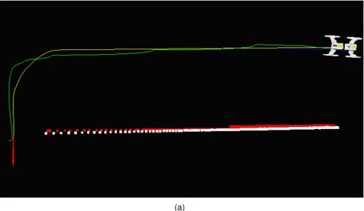
Figure 4.4: (a) Same goal (red arrow) with path generated from different planners, the path of Sbpl lattice is represented in yellow and the Navfn plan is displayed in green, obstacles are displayed in red and laser scanner hits in white
at the expense of computation time, if the computation was the key issue the option should rely in the faster Navfn planner. In sum the global planner supervisory node adds another layer of flexibility to the whole navigation system by allowing the online exchange of global planner algorithm.
4.5
Local Trajectory generation
For the local trajectory generation an instance of the trajectory roll out (Gerkey and Konolige, 2008) is used, where as previously explained in Chapter (2) the idea is to sample the robot control space, then simulate what would be the position of the robot if the sampled velocity was applied for a short period of time. The velocity control space is divided into three componentsdxrepresents forward motion,dyis the side motion component, anddθrepresents the turn in place velocity. Each of this sampled velocities will be carried over the entire forward simulation period given the acceleration limits of the robot and generate a trajectory that will be scored given a certain metric. Then, the one with the lowest cost will be picked to be transmitted to the robot base in (dx,dy,dθ) format.
One limitation of the original roll out algorithm is that it does not encompass the requirements of robots with quasi-omnidirectional locomotion and dynamic footprints. To cater to this needs several modifications were made to the original software that will be summarized in the paragraphs below.