MULTIPATH MITIGATION IN TIME-DELAY
ESTIMATION VIA TENSOR-BASED
TECHNIQUES FOR ANTENNA
ARRAY-BASED GNSS RECEIVERS
DANIEL VALLE DE LIMA
DISSERTAÇÃO DE MESTRADO EM ENGENHARIA ELÉTRICA DEPARTAMENTO DE ENGENHARIA ELÉTRICA
UNIVERSIDADE DE BRASÍLIA
FACULDADE DE TECNOLOGIA
DEPARTAMENTO DE ENGENHARIA ELÉTRICA
MULTIPATH MITIGATION IN TIME-DELAY
ESTIMATION VIA TENSOR-BASED
TECHNIQUES FOR ANTENNA
ARRAY-BASED GNSS RECEIVERS
DANIEL VALLE DE LIMA
Orientador: PROF. DR.-ING. JOÃO PAULO C. L. DA COSTA, ENE/UNB, TU ILMENAU, FRAUNHOFER IIS
DISSERTAÇÃO DE MESTRADO EM ENGENHARIA ELÉTRICA
UNIVERSIDADE DE BRASÍLIA
FACULDADE DE TECNOLOGIA
DEPARTAMENTO DE ENGENHARIA ELÉTRICA
MULTIPATH MITIGATION IN TIME-DELAY
ESTIMATION VIA TENSOR-BASED
TECHNIQUES FOR ANTENNA
ARRAY-BASED GNSS RECEIVERS
DANIEL VALLE DE LIMA
DISSERTAÇÃO DE MESTRADO ACADÊMICO SUBMETIDA AO DEPARTAMENTO DE ENGENHARIA ELÉTRICA DA FACULDADE DE TECNOLOGIA DA UNIVERSIDADE DE BRASÍLIA, COMO PARTE DOS REQUISITOS NECESSÁRIOS PARA A OBTENÇÃO DO GRAU DE MESTRE EM ENGENHARIA ELÉTRICA.
APROVADA POR:
Prof. Dr.-Ing. João Paulo C. L. da Costa, ENE/UnB, TU Ilmenau, Fraunhofer IIS Orientador
Prof. Dr. Ugo Silva Dias, ENE/UnB Examinador interno
Prof. Dr.-Ing. Felix Antreich, DETI/UFC Examinador externo
FICHA CATALOGRÁFICA
DANIEL VALLE DE LIMAMultipath Mitigation in Time-Delay Estimation via Tensor-based Techniques for Antenna Array-based GNSS receivers
2017xv, 63p., 201x297 mm
(ENE/FT/UnB, Mestre, Engenharia Elétrica, 2017) Dissertação de Mestrado - Universidade de Brasília
Faculdade de Tecnologia - Departamento de Engenharia Elétrica
REFERÊNCIA BIBLIOGRÁFICA
DANIEL VALLE DE LIMA (2017) Multipath Mitigation in Time-Delay Estimation via Tensor-based Techniques for Antenna Array-based GNSS receivers. Dissertação de Mes-trado em Engenharia Elétrica, Publicação xxx/AAAA, Departamento de Engenharia Elétrica, Universidade de Brasília, Brasília, DF, 63p.
CESSÃO DE DIREITOS
AUTOR: Daniel Valle de Lima
TÍTULO: Multipath Mitigation in Time-Delay Estimation via Tensor-based Techniques for Antenna Array-based GNSS receivers.
GRAU: Mestre ANO: 2017
É concedida à Universidade de Brasília permissão para reproduzir cópias desta dissertação de Mestrado e para emprestar ou vender tais cópias somente para propósitos acadêmicos e cientí-ficos. Ao autor se reserva outros direitos de publicação e nenhuma parte desta dissertação de Mestrado pode ser reproduzida sem a autorização por escrito do autor.
____________________________________________________ Daniel Valle de Lima
Agradecimentos
Aos meus pais, pelo apoio e amor incondicional que me deram.
Ao meu irmão, por seu amor fraterno e por nossas discussões filosóficas.
Ao meu orientador de Graduação, Dr. Antônio José Martins, pelas aulas de Electromagne-tismo e por possibilitar minha formação inicial como Engenheiro Eletricista.
Ao meu orientador de Mestrado, Dr.-Ing. João Paulo Lustosa, por ser um exemplo a ser se-guido de realização acadêmica, proatividade e curiosidade científica. Sou grato também por sua liderança e orientação, além do investimento de tempo, confiança, e paciência necessária para guiar minha formação como engenheiro e pesquisador.
Àqueles meus colegas que também escolheram o árduo caminho da Engenharia. Sempre podemos aprender com os companheiros de batalha.
Aos professores que me fizeram merecer o título de Engenheiro.
Ao Dr.-Ing. Antreich e o Dr. Dias por fazerem parte da banca e pela crítica que me ajudou a aperfeiçoar esta dissertação.
Dedicatória
Para meus pais.
Resumo
Motivação
Tradicionalmente sistemas satélites de navegação global, em inglês Global Navigation Satellite System(GNSS), como o sistema de posicionamento global, do inglêsGlobal Positi-oning System(GPS), Galileo, o GNSS da União Européia, GLONASS, o GNSS da Federação Russa, ou o BeiDou, o GNSS da República Popular da China, foram concebidos para aplica-ções militares como sistemas de misseis guiados e para aplicaaplica-ções civis como decolagem e pouso de aviões civis. Na aviação civil, sistemas de apoio assistidos por bases terrestres que providenciam informações complementares ao do GNSS aumentam a precisão para sistemas de segurança crítica. Nos últimos anos a quantidade de aplicações de GNSS têm aumentado drasticamente. Por exemplo, autoridades de pesca utilizam GNSS para fazer a localização e rastreio automático em tempo real de barcos pesqueiros para garantir assim o gerenciamento sustentável de fontes de pesca [1]. Outra aplicação de GNSS é o rastreio de caminhões para poder saber o estado da carga em tempo real. Em aplicações de trânsito, o GNSS pode ser utilizado para efetuar um pedágio automatico [2] e para veículos autônomos que exigem al-tos padrões de precisão e segurança. No contexto de veículos autônomos, o veículo deve ser capaz de sensorear o ambiente e os dados processados para atingir o padrão de segurança necessário. Apesar de veículos autônomos contarem com uma quantidade grande de senso-res para controle automático de velocidade de cruzeiro, do inglêsAutomatic Cruise Control (ACC), receptores GNSS exercem uma função essencial [3] devido à cobertura quase ubíqua de todas as regiões do planeta. Finalmente, em agricultura de precisão, também conhecido por agricultura por satélite, GNSS é usado para melhorar, por exemplo, a precisão com que é feita a adubagem e permite o uso de veículos agrícolas automatizados em qualquer hora do dia [4]. Assim, na agricultura de precisão, tanto máquinas quanto recursos químicos podem ser usados de forma mais segura e eficiente.
GNSS depende da estimação do atraso para estimar a posição do usuário. Isto é feito fazendo a correlação do sinal recebido com réplicas para separá-lo o sinal de cada satélite e estimar o atraso. Como componentes de multipercurso são cópias atrasadas do sinal original, estes alteram a função de correlação cruzada, assim gerando erros na estimação de atraso.
alta ordem, do inglêsHigher-Order Singular Value Decomposition(HOSVD), de posto uni-tário [5], e propomos dois esquemas tensoriais para mitigação de multipercurso e estimação de atraso, para qual o esquema baseado em HOSVD é usado para comparação.
Modelo de Dados
O modelo de dados do receptor tensorial supõe um arranjo receptor de M elementos,
observandoDsatélites visíveis, comLdsinais vindo de cadad-ésimo satélite. ComLd = 1
para o componente de linha de visada, do inglês Line-of-Sight (LOS), e Ld > 1 para os
componentes de multipercurso. ColetandoN amostras a cadak-ésimo período de código,
X[k] =
D
X
d=1
Ad[k]Γd[k]Cd[k] +N[k] =A[k]Γ[k]C[k] +N[k]∈CM×N, (1)
em que Ad[k] = [a(φd,1), . . . ,a(φd,Ld)] ∈ C
M×Ld é a matriz que concatena em suas
co-lunas os vetores de direção dos Ld sinais. Γd[k] = diag{γd} = diag{[γd,1, . . . , γd,Ld]} ∈
CLd×Ld é uma matriz diagonal que contém as amplitudes complexas dos sinais. C
d[k] =
[cd[τd,1], . . . ,cd[τLd]
T
∈ RLd×N concatena em suas linhas o código pseudo-aleatório
amos-trado com atraso τd,ld, ld = 1, . . . , Ld. N[k]é ruído gaussiano branco aditivo. A ordem do
modelo éL=PDd=1Ld.
Aplicando o operadorvec{·}a (1) para transformá-lo num vetor e aplicando a proprie-dade descrita na subseção 2.2.4,
vec{X[k]}= vec{A[k]Γ[k]C[k] +N[k]}= vec{A[k] diag{γ[k]}C[k] +N[k]},
= (C[k]T⋄A[k])γ[k] + vec{N[k]}. (2)
Concatenando todos osK períodos de código amostrados na direção das colunas é pos-sível omitir o índicek:
˜
X= (CT⋄A)˜Γ+ ˜N= ˜X0+ ˜N∈CM N×K, (3)
em que X˜0 é o sinal recebido sem ruído e Γ˜ = [γ[1]. . . ,γ[K]] ∈ CL×K concatena as
amplitudes complexas.
A transposta deX˜0possui a mesma estrutura que o desdobramento do primeiro modo de um tensor de recepção sem ruídoX0:
[X0](1) = ˜XT0 = ˜Γ
T
Dobrando (4) num tensor e considerando o caso com ruído:
X =X0+N =I3,L×1Γ˜T×2CT×3A+N ∈CK×N×M. (5)
Para separar o sinal do d-ésimo satélite dos outros, um banco correlator é aplicado ao
código pseudo-aleatório usando o produto de modo-2. Um banco correlator é uma matriz Qdque concatenaQréplicas deslocadas da sequência pseudo-aleatóriacd∈RN com atraso
τq, q= 1, . . . , Q:
Qd=
h
cd[τ1] · · · cd[τQ]
i
∈RN×Q. (6)
Como a aplicação direta do banco correlator torna o ruído colorido, um banco compri-mido é calculado utilizando a decomposição em valores singulares econômica àQd[22]:
Qd=Qω,dΣVH, (7)
em que o banco comprimido éQω,d ∈CN×Q.
Aplicando o banco correlator comprimido à (5) para extrair o sinal dod-ésimo satélite:
Yd =X ×2 QTω,d =I3,L×1Γ˜Td×2(CdQω,d)T×3Ad+Nω ∈CK×Q×M. (8)
O desdobramento do terceiro modo de (8) é
[Yd](3) =Ad(˜ΓTd⋄(CdQω,d)T)T+ [Nω](3) ∈CM×KQ. (9)
Estado-da-Arte para Estimação de Atraso
A técnica estado-da-arte estudado neste dissertação é um autofiltro de alta ordem com pré-processamento usando média frente-costas [16], do inglês Forward-Backward Avera-ging (FBA), e suavização espacial expandida [18, 19], do inglês Expanded Spatial Smo-othing (ESPS), como pode ser visto na Figura 3.1. A primeira etapa desta técnica é de pré-processamento em que FBA é aplicado a (9):
Z=h[Yd](3) ΠM[Yd]∗(3)ΠKQ
i
∈CM×2KQ, (10)
matriz de seleção
JlS =
h
0MS×lS−1 IMS 0MS×LS−1
i
∈RMS×M, (11)
paralS = 1, . . . , LS.
Usando as matrizes de seleção, suavização espacial é aplicado a (10):
W=hJ1Z · · · JLSZ
i
∈CMS×2LSKQ, (12)
e (12) é dobrado de volta para um tensor de quarta ordemZESPS ∈C2K×Q×MS×LS. Esta é a suavização espacial expandida.
Em seguida é aplicada uma decomposição em valores singulares de alta ordem, em inglês Higher-Order Singular Value Decomposition(HOSVD) àZESPS:
ZESPS =R×1U(1)×2U(2)×3U(3)×4U(4), (13)
em que R ∈ C2K×Q×MS×LS é o tensor núcleo eU(1) ∈ C2K×2K, U(2) ∈ CQ×Q, U(3) ∈
CMS×MS, e U(4) ∈ CLS×LS são as matrizes singulares contendo os vetores singulares dos
desdobramento de (8) em cada modo, respectivamente.
Supondo que os componentes de sinais LOS são dominantes, os vetores singulares domi-nantes do primeiro, terceiro, e quarto modo de ZESPS são mais correlatados ao componente LOS. Portanto [5] propôs o seguinte autofiltro:
qESPS =
ZESPS×1(u(1)1 )
H
×3(u(3)1 )
H
×4(u(4)1 )
H
ΣVH, (14)
em queΣVHfoi calculado em (7).
Para estimação do atraso, uma interpolação de spline cúbico é aplicado ao valor absolute de (14) para criar uma função de custoF(τ). A variávelτ que maximizaF(τ)é
ˆ
τLOS = arg max
τ {F(τ)}. (15)
Técnicas Tensoriais Propostas
Esquema tensorial por estimação da matriz de direção e fatorização
Khatri-Rao (DoA/KRF)
Após o pré-processamento de (9) usando FBA e SPS, estimação de DoA é aplicado a (12) para estimar a matriz-fator de direção de chegadaAˆd. Como[Yd](3) ≈Ad(˜ΓT
⋄(CdQω,d)T)T,
o produto da pseudo-inversa deAˆdpor[Yd](3)é ˆ
A+d[Yd](3) ≈Aˆ+dAd(˜ΓTd⋄(CdQω,d)T)T ≈(˜ΓTd⋄(CdQω,d)T)T. (16)
Em seguida, uma KRF é aplicado a (16) para encontrar as matrizes-fatorΓˆ˜d eCˆdQω,d.
Com o código separado é possível determinar a correlação usandoΣVH: ˆ
CdQd= ˆCdQω,dΣVH. (17)
Por causa da possibilidade de ambiguidade de permutação na estimação do DoA ou na KRF, um esquema de seleção é aplicado para descobrir qual linha de (17) contém a correla-ção com o componente de linha de visada. Dois esquemas de selecorrela-ção foram propostos.
O primeiro esquema de seleção é baseado em potência e supõe que o componente LOS do sinal é o de maior potência, isto é
lLOS= max
ld k
(ˆ˜Γd)ld,·k2, (18)
e interpolação de spline cúbica é aplicada para estimar o atrasoτˆapenas da linha selecionada de (17).
No segundo esquema de seleção, a interpolação de spline cúbica é aplicada a todas as linhas de (17) para estimar os atrasos dos componentes LOS e NLOS num vetor τˆ e supõe que o componente LOS do sinal é o de menor atraso destes, portanto
ˆ
τLOS = min
τ {τˆ}. (19)
Esquema tensorial por filtragem ProKRaft
O segundo esquema tensorial utiliza um desdobramento Hermitiano, calculado a partir do tensor de recepção, cuja propriedade de simetria dual [6] é explorada por um algoritmo que alterna entre a solução do problema ortogonal de Procrustes, do inglêsOrthogonal Pro-crustes Problem (OPP), e fatorização Khatri-Rao de mínimos quadrados, do inglês Least Squares Khatri-Rao Factorization (LSKRF), para estimar iterativamente as matrizes-fator do canal. Estas são então usadas para separar o código de cada componente incidente.
em queRC ∈RLd×Ld é a matriz de covariância dos componentes LOS e NLOS de sinal do
satélited.
ComoRC ≈ILd(20) pode ser aproximado como
Rmm ≈(Ad⋄Γ˜dT)(Ad⋄Γ˜Td)
H
=YH, (21)
eYHé o desdobramento Hermitiano deYd. ComoYHpossui a propriedade de simetria dual é possível definir uma matriz-raizY
1 2
H ∈CM K×Ldtal que: YH=Y
1 2
H(Y
1 2
H)H. (22)
Usando a decomposição em valores singulares, do inglêsSingular Value Decomposition (SVD), de (21), YH = UYΣYVHY, é possível calcular uma estimativa paraY
1 2
H. Usando os vetores singulares esquerdos associados ao subespaço de sinal, U[Ld]
Y ∈ CM K×Ld, os valo-res singulavalo-res associados ao subespaço do sinal, Σ[Ld]
Y ∈ CLd×Ld, e uma matriz de rotação unitáriaWH∈CLd×Ld:
ˆ Y
1 2
H =U[
L]
Y Σ[
L]
Y WH = (A⋄Γ˜T) (23)
=FWH=G.
MapearF paraG usandoWH é conhecido como o problema ortogonal de Procrustes. Uma solução conhecida para este problema é aplicar a SVD aFGHe usar os vetores singu-lares desta decomposição para estimarWH[30]:
FGH=UPΣPVHP
WH=UPVHP. (24)
Um algoritmo que alterna entre (23) e (24) pode iterativamente estimarAˆdeΓˆ˜d.
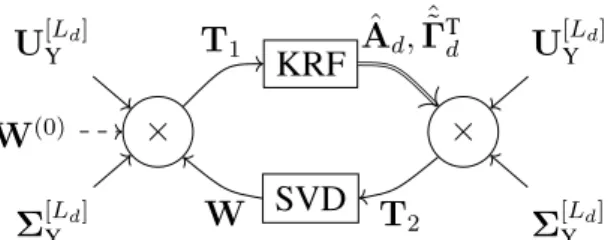
Como pode ser visto na Figura 3.3, o algoritmo inicia calculando os valores e vetores singulares de (20) e inicializandoW(0) =I
Ld.
WH é usado para calcular T1 = U[Ld]
Y Σ[
Ld]
Y WH. Aplicando LSKRF à T1 se calcula
estimativas para Aˆd e Γˆ˜d, que são utilizadas para calcularT2 = ( ˆAd⋄Γˆ˜d)U[Ld]
Y Σ[
Ld]
Y . A SVD deT2 fornece as matrizes de vetores singularesUPeVPusadas para atualizarWH. O processo se repete até a convergência.
Com a estimativa das matrizes-fator do canal, a filtragem é feita calculando o produto modo-ncom a pseudoinversa das matrizes-fator estimadas:
ˆ
CdQω,d =Yd×1(ˆ˜Γd)+×3( ˆAd)+, (25)
componentes LOS e NLOS do sinal. Cada l-ésimo código se acumula em cada vetor
(ˆCdQω,d)l,·,l.
Assim como no esquema anterior proposto, pode haver ambiguidades de permutação, e um esquema de seleção igual ao descrito anteriormente é utilizado para selecionar o compo-nente de sinal LOS.
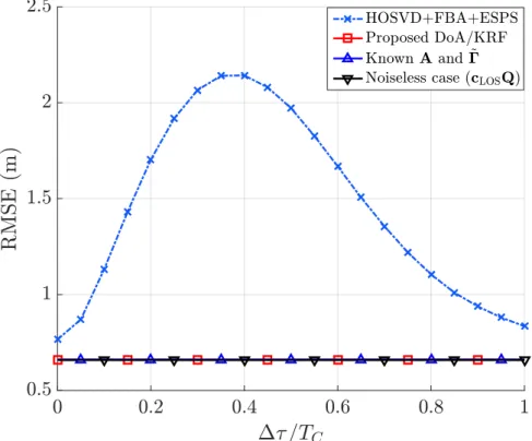
Simulação
É considerado o seguinte cenário sob simulação: é utilizado um arranjo retangular uni-forme, do inglês Uniform Linear Array(ULA), centro-hermitiano comM = 8elementos e espaçamento de meio comprimento de onda. O sinal GNSS é um código pseudo aleatório C/A de GPS de D satélites, com portadora de frequência fc = 1575,42MHz, largura de
bandaB = 1,023 MHz, e duração dechipTC = 1/B = 977,52ns, com N = 2046
amos-tras coletadas a cada k-ésimo período de código durante K = 30 períodos, cada um com duração de∆t= 1ms.
Além do sinal LOS com atrasoτLOS, há um componente NLOS (L= 2) com atrasoτLOS e diferença de azimute de∆φ. O atraso entreτLOSeτNLOSé tal queτNLOS =τLOS+ ∆t. Para SPS/ESPS o arranjo é dividido emLS = 5subarranjos comMS = 4elementos cada.
As fases do sinalarg{γ} ∼U[0,2π]independentes e identicamente distribuídos. Para as
simulações do esquema DoA/KRF, as fases se mantém constante durante todo a amostragem. Para as simulações do esquema ProKRaft, as fases mudam a cada período de código. O número de correlatores no banco é Q = 11igualmente espaçados entre −TC eTC. O sinal
LOS é selecionado utilizando (18). A razão portadora ruído é de48dB-Hz, resultando numa razão sinal-ruído pós-correlação de SNRpós ≈15dB.
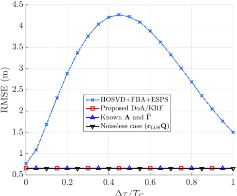
A simulação é de Monte Carlo com 1000 iterações. As curvas são o erro quadrático médio multiplicado por c = 299792458 m/s, expressas em metros, para diferentes∆τ. Os
resultados são comparados com a filtragem com conhecimento a priori do canal (A e Γ˜ conhecidos) e a correlação direta sem ruído do sinal LOS com o banco correlator.
0 0.2 0.4 0.6 0.8 1
"==TC
0.5 1 1.5 2 2.5 R M S E (m ) HOSVD+FBA+ESPS Proposed DoA/KRF KnownAand ~!
Noiseless case (cLOSQ)
(a) DoA/KRF paraD= 1,∆φ=π/3
0 0.2 0.4 0.6 0.8 1 "==TC
0.5 1 1.5 2 2.5 3 3.5 4 4.5 R M S E (m ) HOSVD+FBA+ESPS Proposed DoA/KRF KnownAand ~!
Noiseless case (cLOSQ)
(b) DoA/KRF paraD= 1,∆φ=π/4
0 0.2 0.4 0.6 0.8 1 "==TC
0.6 0.7 0.8 0.9 1 1.1 1.2 1.3 1.4 R M S E (m ) HOSVD+FBA+ESPS Proposed DoA/KRF KnownAand ~!
Noiseless case (cLOSQ)
(c) DoA/KRF paraD= 1,∆φ=π/6
0 0.2 0.4 0.6 0.8 1
"==TC
0.5 1 1.5 2 2.5 R M S E (m ) HOSVD+FBA+ESPS Proposed DoA/KRF KnownAand ~!
Noiseless case (cLOSQ)
(d) DoA/KRF paraD= 2,∆φ=π/3
0 0.2 0.4 0.6 0.8 1
"==TC
0.5 1 1.5 2 2.5 R M S E (m ) HOSVD+FBA+ESPS Proposed DoA/KRF KnownAand ~!
Noiseless case (cLOSQ)
(e) DoA/KRF paraD= 3,∆φ=π/3
0 0.2 0.4 0.6 0.8 1
"==TC
0.6 0.65 0.7 0.75 0.8 R M S E (m ) HOSVD+FBA+ESPS DoA/KRF (SE/LSKRF)
KnownAand ~!
ProKRaft (2 iterations)
(f) ProKRaft paraD= 1,∆φ=π/3
0 0.2 0.4 0.6 0.8 1
"==TC
0.6 0.7 0.8 0.9 1 1.1 1.2 1.3 R M S E (m ) HOSVD+FBA+ESPS DoA/KRF (SE/LSKRF) KnownAand ~!
ProKRaft (2 iterations)
(g) ProKRaft paraD= 1,∆φ=π/4
0 0.2 0.4 0.6 0.8 1
"==TC
0.65 0.7 0.75 0.8 0.85 R M S E (m ) HOSVD+FBA+ESPS DoA/KRF (SE/LSKRF)
KnownAand ~!
ProKRaft (2 iterations)
(h) ProKRaft paraD= 1,∆φ=π/3
Abstract
Traditionally Global Navigation Satellite Systems (GNSS) such as Global Positioning System (GPS), Galileo, also known as the European GNSS, GLONASS, also known as the Russian GNSS, or BeiDou, also known as the Chinese GNSS, are intended for military ap-plications such as missile guiding-system and for takeoff and landing of civilian airplanes. In case of civilian aviation, Ground-Based Augmentation System (GBAS) supports local augmentation for safety-critical systems. However, in the last years, the amount of GNSS applications has dramatically increased. For instance, fishing authorities can use GNSS to automatically locate in real-time by satellites the fishing ships in order to guarantee the sus-tainable management of the fishing commonwealth [1]. Another application of GNSS is to track trucks in order to know the status of the load in real-time. In traffic related applications, GNSS can be used for an automatic toll system [2] and for autonomous vehicles that require high standards of security and precision. In the context of autonomous driving, the environ-ment should be sensed by the vehicle and the measured data processed in order to achieve such standards. Although autonomous vehicles count on an extensive amount of sensors to perform Adaptive Cruise Control (ACC), GNSS receivers play an essential role [3] due to its ubiquity covering almost all areas of the planet. Finally, in precision farming, also known as satellite farming, GNSS is employed to improve, for instance, precision of fertilization and also to allow the usage of expensive agriculture vehicles 24 hours a day [4]. Therefore, with precision agriculture, both machinery and chemicals can be used in a safer and more efficient fashion.
GNSSs rely on time-delay estimation to estimate a user’s position. This is done by cor-relating the incoming signal with replica sequences to separate each satellite and perform time-delay estimation. Since multipath components are delayed copies of the original sig-nal, this affects the cross-correlation function, thus impacting time-delay estimation.
In this thesis, we study a state-of-the-art approach for multipath mitigation time-delay estimation algorithm based on the rank-one Higher-Order Singular Value Decomposition (HOSVD) eigenfilter [7], and propose two tensor-based schemes for multipath mitigation and time-delay estimation, for which the HOSVD-based scheme is a basis of comparison.
CONTENTS
1 INTRODUCTION. . . 1
2 CONCEPTS ONTENSORCALCULUS ANDDATAMODEL . . . 3
2.1 NOTATION... 3
2.2 MATRIXCALCULUS ... 4
2.2.1 KRONECKER PRODUCT... 4
2.2.2 KHATRI-RAO PRODUCT... 5
2.2.3 OUTER PRODUCT ... 5
2.2.4 THEvec{·}OPERATOR... 5
2.2.5 THEunvec{·}OPERATOR... 6
2.3 TENSORCALCULUS ... 6
2.3.1 TENSORS... 6
2.3.2 n-MODE UNFOLDING... 7
2.3.3 n-MODE PRODUCT... 8
2.3.4 PARAFAC MODEL ... 8
2.3.5 HIGHER-ORDERSVD ... 9
2.3.6 DUAL-SYMMETRIC TENSORS... 11
2.4 DATAMODEL... 12
2.4.1 PRE-CORRELATION DATA MODEL... 13
2.4.2 POST-CORRELATION DATA MODEL ... 15
2.4.3 UNIFORM LINEARARRAY... 16
3 TENSOR-BASED APPROACHES TOTIME-DELAY ESTIMATION. . . 19
3.1 STATE-OF-THE-ARTTENSOR-BASEDTIME-DELAY ESTIMATION... 19
3.1.1 FORWARD-BACKWARD AVERAGING AND EXPANDED SPATIAL SMO -OTHING... 20
3.1.2 HIGHER-ORDERSVD EIGENFILTERING ... 20
3.1.3 TIME-DELAY ESTIMATION ... 21
3.2 PROPOSED DOA ESTIMATION ANDKRF APPROACH... 21
3.2.1 ESTIMATION OF DOAFACTOR MATRIX... 22
3.2.2 PR CODE AND COMPLEX AMPLITUDE ESTIMATION VIAKHATRI-RAO FACTORIZATION... 22
3.3 PROCRUSTES ESTIMATION AND KHATRI-RAO FACTORIZATION (PRO
-KRAFT)FILTERING... 24
3.3.1 SIMULTANEOUSDOAAND AMPLITUDE FACTOR MATRIX ESTIMATION.. 24
3.3.2 LOS TIME-DELAY ESTIMATION... 26
4 SIMULATIONS. . . 27
4.1 PROKRAFT FILTERING TIME-DELAY ESTIMATION... 29
4.2 SIMULATION WITH MULTIPLE SATELLITES... 30
4.3 EFFECTS OF IMPROPER MODEL ORDER ESTIMATION... 30
4.3.1 UNDERESTIMATION ... 31
4.3.2 OVERESTIMATION ... 32
5 CONCLUSION. . . 40
LISTA OF FIGURES
2.1 Third-order tensor PARAFAC decomposition... 9
2.2 Singular Value Decomposition ... 10
2.3 SVD generalized using then-mode product ... 10
2.4 Higher-Order SVD of a third-order tensorX ... 11
2.5 Uniform Linear Array with∆spacing ... 16
2.6 Wavefront incidence on adjacent array elements ... 17
3.1 Block diagram of the state-of-the-art HOSVD eigenfilter-based time-delay estimation approach... 21
3.2 Block Diagram of the proposed DoA/KRF time-delay estimation approach .... 24
3.3 Block Diagram of the proposed ProKRaft factor matrices estimation approach 26 4.1 Simulation results for DoA/KRF,D= 1,∆φ=π/3... 28
4.2 Simulation results for DoA/KRF,D= 1,∆φ=π/4... 29
4.3 Simulation results for DoA/KRF,D= 1,∆φ=π/6... 30
4.4 Simulation results for ProKRaft,D= 1,∆φ =π/3... 31
4.5 Simulation results for ProKRaft,D= 1,∆φ =π/4... 32
4.6 Simulation results for ProKRaft,D= 1,∆φ =π/6... 33
4.7 Simulation results for DoA/KRF,D= 2,∆φ=π/3... 33
4.8 Simulation results for DoA/KRF,D= 3,∆φ=π/3... 34
4.9 Simulation results for DoA/KRF,D= 4,∆φ=π/3... 34
4.10 Simulation results for DoA/KRF,D= 1,∆φ=π/3,L1 = 3,Lˆ1 = 3... 35
4.11 Simulation results for ProKRaft,D= 1,∆φ =π/3,L1 = 3,Lˆ1 = 3... 35
4.12 Simulation results for DoA/KRF,D= 1,∆φ=π/3,L1 = 2,Lˆ1 = 1... 36
4.13 Simulation results for DoA/KRF,D= 1,∆φ=π/3,L1 = 3,Lˆ1 = 2... 36
4.14 Simulation results for ProKRaft,D= 1,∆φ =π/3,L1 = 2,Lˆ1 = 1... 37
4.15 Simulation results for ProKRaft,D= 1,∆φ =π/3,L1 = 3,Lˆ1 = 2... 37
4.16 Simulation results for DoA/KRF,D= 1,∆φ=π/3,L1 = 2,Lˆ1 = 3... 38
4.17 Simulation results for DoA/KRF,D= 1,∆φ=π/3,L1 = 3,Lˆ1 = 4... 38
4.18 Simulation results for ProKRaft,D= 1,∆φ =π/3,L1 = 2,Lˆ1 = 3... 39
Chapter 1
Introduction
Originally Global Navigation Satellite Systems (GNSS) such as Global Positioning Sys-tem (GPS) were intended for military applications, such as missile guiding-sysSys-tems, and for takeoff and landing of civilian airplanes. In case of civilian aviation, Ground-Based Aug-mentation System (GBAS) supports local augAug-mentation for safety-critical systems. In the last years, the amount of GNSS applications has increased dramatically. For instance, GNSS can be used for automatic toll systems [2] and for autonomous vehicles that require high standards of security and precision [3]. In precision farming, GNSS is employed to improve, for instance, precision application of fertilization and also to allow the usage of expensive agriculture machinery 24 hours a day [4].
In order to compute the position on the earth, a GNSS receiver uses the time-delays of line-of-sight (LOS) components from at least four satellites. However, due to the geometry of the propagation environment, caused, for instance, by trees, poles, lamps and buildings, reflections from the LOS signal can occur creating multipath components, which are non-line-of-sight (NLOS) components. As a consequence, the multipath components interfere with the received LOS signal component. In practice, the quality of the ranging data provided by a GNSS receiver largely depends on the synchronization error, that is, on the accuracy of the propagation time-delay estimation of the LOS signal. In case the LOS signal is corrupted by several superimposed delayed replicas (reflective, diffractive, or refractive multipath), the estimation of the propagation time-delay and thus the position can be severely degraded using state-of-the-art GNSS receivers [8, 9, 10].
Several techniques have been proposed in the literature for solving the multipath problem in GNSS using one single-polarization antenna, e.g. [11, 12], but their capabilities are not sufficient for safety-critical applications (SCA) or liability critical applications (LCA). Thus, multi-antenna systems became the focus of research and technological development of mul-tipath mitigation for SCA and LCA [13, 14]. The current state-of-the-art tensor-based multi-path mitigation techniques applied to time-delay estimation [5] is based on HOSVD [15] ei-genfiltering with Forward-Backward Averaging (FBA) [16, 17], and Expanded Spatial Smo-othing (ESPS) [18, 19].
In this thesis we propose two new tensor-based time-delay estimation approach robust against multipath components. Our first approach starts by utilizing a direction of arrival (DoA) estimation technique on the post-correlated received tensor signals in order to recons-truct the DoA-related factor matrix. Next, the remaining factor matrices can be estimated by using Khatri-Rao factorization (KRF). Given the estimated factor matrix corresponding to the post-correlated pseudo-random (PR) sequences, the time-delay estimation can be per-formed for each LOS and NLOS signal component. Therefore, we also incorporate two proposed selection schemes in our framework in order to estimate the time-delay of the LOS signal component: one based on the signal power and another one selecting the smallest esti-mated time-delay. The second approach utilizes a Procrustes estimation and Khatri-Rao fac-torization (ProKRaft) technique to estimate the DoA- and complex amplitude-related factor matrices which are then used to filter and recover the post-correlated PR sequences. Again, a selection scheme is employed to estimate the time-delay of the LOS signal component.
Chapter 2
Concepts on Tensor Calculus and Data
Model
While matrix operations such as eigenvalue and singular value decompositions are well known, certain specific matrix operations which are used in this thesis are more rarely seen and their usage is necessary for the tensor operations used for tensor-based filtering tech-niques and how the tensor-based GNSS receiver is modeled in this thesis. In this chapter, the notation used in this thesis is introduced in Section 2.1, followed by matrix operations in Section 2.2, the tensor operations and how they relate to the matrix operations in Section 2.3, and finally the data model for the tensor-based GNSS receiver before and after correlation with the correlator bank.
2.1 Notation
Scalars are represented by italic letters (a, b, A, B), vectors by lowercase bold letters (a,b), matrices by uppercase bold letters (A,B), and tensors by uppercase bold calligraphic letters (A,B).
The superscriptsT, ∗, H, −1, and+ denote the transpose, conjugate, conjugate transpose
(Hermitian), inverse, and pseudo-inverse of a matrix, respectively.
For a matrixA ∈ CM×N, the element in the m-th row andn-th column is denoted by
am,n, its m-th row is denoted by (A)m,·, and its n-th column is denoted by (A)·,n. The
2-norm of a matrixAis denoted bykAk2.
For a matrixA ∈ CM×N with M < N, the diag{·} operator extracts the diagonal is
defined as
diag{A},
a1,1
a2,2
.. . aM,M . (2.1)
The n-th mode unfolding of the tensorA is denoted by [A](n). The n-mode product
between a tensorA and a matrixB is denoted byA×nB. TheN-th order identity tensor
of sizeL×. . .×Lis denoted byIN,L.
For two N-th order tensor A and B, both of size I1 × I2 ×. . . ×IN, composed of
individual scalar elements ai1,i2,...,iN andbi1,i2,...,iN, respectively, its inner product is denoted
byhA,Bi, and is defined as
hA,Bi,
I1
X
i1=1
I2 X i2=1 . . . IN X
iN=1
ai1,i2,...,iNbi1,i2,...,iN. (2.2)
The norm of a tensorA, denoted bykAkF, is the Frobenius norm defined as
kAkF,
p
hA,Ai. (2.3)
2.2 Matrix Calculus
In this section four matrix operations are presented. The first two, the Kronecker and Khatri-Rao products are straightforward, the latter two have important properties that are used in the data model used in this work.
2.2.1 Kronecker product
Given two matricesA ∈ CI×J andB ∈ CK×Ltheir Kronecker product, denoted by⊗,
is defined as:
A⊗B,
a1,1B · · · a1,JB
..
. . .. ... aI,1B · · · aI,JB
∈C
IK×J L
2.2.2 Khatri-Rao product
Given two matricesA ∈ CI×R andB
∈ CK×Rtheir Khatri-Rao product, denoted by
⋄, is defined as:
A⋄B ,h(A)·,1⊗(B)·,1 · · · (A)·,R⊗(B)·,R
i
∈CIJ×R. (2.5)
2.2.3 Outer product
The outer product is a special case of the Kronecker product in which the outer product of two vectorsa∈CI andb
∈CJ results in a matrixC
∈CI×J:
a◦b=abT =
a1 .. . aI h
b1 · · · bJ
i (2.6) =
a1b1 · · · a1bJ
..
. . .. ... aIb1 · · · aIbJ
=C∈C
I×J, (2.7)
such that the elements ofCsatisfycij =aibj, i∈ {1, . . . , I}, j ∈ {1, . . . , J}.
The outer product can also be extended into other dimensions. An outer product of three vectors results in a third-order tensor. For example, the outer product of three vectorsa∈CI,
b ∈CJ, andc∈CKresults in a third-order tensorX ∈CI×J×K
a◦b◦c=X ∈CI×J×K, (2.8)
andxijk =aibjck, i∈ {1, . . . , I}, j ∈ {1, . . . , J}, k ∈ {1, . . . , K}holds.
2.2.4 The
vec
{·}
operator
Thevec{·} operator rearranges a matrix into a vector in such a way that its vectors are stacked. For a matrixA∈CM×N,
vec{A}=vecnhA·1 · · · A·N
io (2.9) =
A·1
.. .
A·N
∈
CM N. (2.10)
An important property of thevec{·}operator is that forX = ABCwith A ∈ CI×J, a
diagonal matrixB∈CJ×J, andC
∈CJ×K
vec{X}=vec{ABC}
= (CT⋄A)diag{B} ∈CIK. (2.11)
2.2.5 The
unvec
{·}
operator
Theunvec{·}operator rearranges a vector into a matrix of specified size. For a vector a= [aT1, . . . ,aTN]T ∈CM N,
unvec
M×N {a}= unvecM×N
a1 .. . aN
=ha1 · · · aN
i
∈CM×N. (2.12)
2.3 Tensor Calculus
2.3.1 Tensors
As vectors are generalizations of scalars, and matrices generalizations of vectors, ten-sors are generalizations of matrices but, while matrices are limited to only two dimensions, tensors can have any number of dimensions. Throughout this text the terms scalar, vector and matrix are applied to 0-, 1-, and 2-dimensional structures while the term tensor is only applied to structures with 3 or more dimensions.
In (2.13) we examplify a scalarI ∈C, a vectori∈C3, and an identity matrixI∈C3×3:
I = 1, i=
1 0 0
, I =
1 0 0 0 1 0 0 0 1
while in (2.14) a third-order identity tensorI3,3 ∈C3×3×3is shown:
I3,3 =
0 0 0 0 1 0 0 0 0
0 0 0 0 0 0 0 0 1
1 0 0 0 0 0 0 0 0
. (2.14)
While higher-order tensors can be achieved visualization becomes difficult. A N
-dimensional tensor A ∈ CI1×I2×...×IN can be perceived in “slices” by keeping its first two
indexes fixed while varying the remainingN −2indexes in succession.
For example, by changing the third index of the previously used third-order identity tensorI3,3while fixing the first and second indexes:
(I3,3)·,·,1 =
1 0 0 0 0 0 0 0 0
(I3,3)·,·,2 =
0 0 0 0 1 0 0 0 0
(I3,3)·,·,3 =
1 0 0 0 0 0 0 0 1
. (2.15)
For a fourth-order identity tensorI4,3 ∈C3×3×3×3we get
(I4,3)·,·,1,1 =
1 0 0 0 0 0 0 0 0
(I4,3)·,·,2,1 =
0 0 0 0 0 0 0 0 0
(I4,3)·,·,3,1 =
0 0 0 0 0 0 0 0 0
(2.16)
(I4,3)·,·,1,2 =
0 0 0 0 0 0 0 0 0
(I4,3)·,·,2,2 =
0 0 0 0 1 0 0 0 0
(I4,3)·,·,3,2 =
0 0 0 0 0 0 0 0 0
(2.17)
(I4,3)·,·,1,3 =
0 0 0 0 0 0 0 0 0
(I4,3)·,·,2,3 =
0 0 0 0 0 0 0 0 0
(I4,3)·,·,3,3 =
0 0 0 0 0 0 0 0 1
. (2.18)
2.3.2
n
-mode unfolding
The n-mode unfolding provides a way to represent a tensor as a matrix. This is done
by fixing then-th index while varying the remaining indexes in reverse order, concatenating
these vectors along the n + 1-th dimension, then permutating the order of the dimensions
(circularly) from then-th to then−1-th dimension.
For example, for a third-order tensorA∈C2×2×2we can write
A =
"
5 6 7 8
#
"
1 2 3 4
# . (2.19)
and has the following unfoldings:
[A](1) =
"
1 5 2 6 3 7 4 8
#
, (2.20)
[A](2) =
"
1 3 5 7 2 4 6 8
#
, (2.21)
[A](3) =
"
1 2 3 4 5 6 7 8
#
. (2.22)
For aN-dimensional tensor, A ∈ CI1×...×IN, its n-mode unfolding, [A]
(n), will be of
sizeIn×Πr6=nIr.
2.3.3
n
-mode product
The n-mode product allows for the calculation of the product between a matrix and a tensor by using the n-mode unfolding. For anN-dimensional tensorA ∈ CI1×...×In×...×IN
and a matrixB∈CM×In, then-mode product of these two matrices is denoted byA
×nB.
The resulting tensor is the matrix product of B ·[A](n) folded back into a tensor of size
I1×. . .×M ×. . .×IN.
Alternatively, this can be interpreted as then-mode unfolding of the resulting tensor as the product between the matrixBand the unfolded tensorA:
[A×nB](n)=B·[A](n). (2.23)
2.3.4 PARAFAC model
The PARAFAC model presupposes that a given N-dimensional tensorX ∈ CI1×...×IN
can be decomposed into a summation of a minimum number of rank-one tensorsX(i), i =
1, . . . , L:
X =
L
X
l=1
X(l) =
L
X
l=1
a(1)l ◦. . .◦a(lN), (2.24)
By defining factor matricesA(i) = [a1(i), . . . ,a(1i)]the equation above can be written in terms of the n-mode products of an N-dimensional identity matrix IN,L ∈ RL×...×L and
loading matricesA(i):
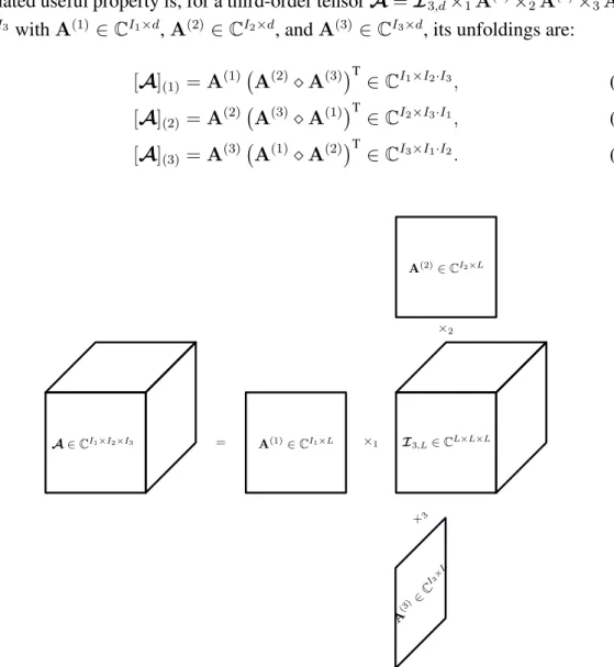
X =IN,L×1A(1)×2A(2). . .×N A(N). (2.25)
A related useful property is, for a third-order tensorA =I3,d×1A(1)×2A(2)×3A(3) ∈
CI1×I2×I3 withA(1)
∈CI1×d,A(2)
∈CI2×d, andA(3)
∈CI3×d, its unfoldings are:
[A](1) =A(1) A(2)⋄A(3)
T
∈CI1×I2·I3, (2.26)
[A](2) =A(2) A(3)⋄A(1)
T
∈CI2×I3·I1, (2.27)
[A](3) =A(3) A(1)⋄A(2)
T
∈CI3×I1·I2
. (2.28)
Figure 2.1: Third-order tensor PARAFAC decomposition
2.3.5 Higher-Order SVD
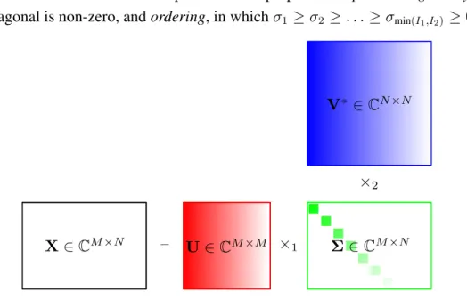
A matrixX∈ CI1×I2 can be decomposed by the Singular Value Decomposition into the
following products:
X=UΣVH, (2.29)
withU∈CI1×I1,Σ
∈CI1×I2, andV
∈CI2×I2.
Uis a unitary matrix containing the left-hand singular vectors and its columns are asso-ciated with the column space of X. Vis a unitary matrix containing the right-hand singular vectors and its rows are associated with the row space of X. Σis a matrix containing the singular valuesσ1, σ2, . . . , σmin(I1,I2)in its diagonal, its columns are multiplied byUand its
rows are multiplied byV∗.
Figure 2.2: Singular Value Decomposition
To generalize the SVD to anN-th order tensor the relations described above have to be retained while extending to tensors. For more than two dimensions the transpose operation does not make sense. To achieve the SVD without relying on the transpose operation while preserving the relations betweenU,V, andΣ, then-mode product described previously can be employed:
X =UΣVH
=Σ×1U×2V∗
=Σ×1U(1)×2U(2), (2.30)
with U(1) = U and U(2) = V∗. Σpossesses the properties of pseudodiagonality, that is only its diagonal is non-zero, andordering, in whichσ1 ≥σ2 ≥. . .≥σmin(I1,I2) ≥0.
Figure 2.3: SVD generalized using then-mode product
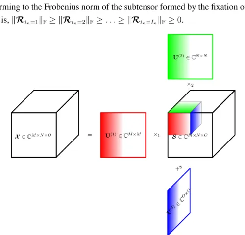
Generalizing the SVD to anN-th order tensorX ∈ CI1×I2×...×IN in terms of ann-mode
product:
in which each U(n)
∈ CIn×In is a unitary matrix that makes linear combinations of the
subtensor formed by keeping the n-th index of R ∈ CI1×I2×...×IN fixed. This is known as
the Higher-Order SVD [15].
The tensor R ∈ CI1×I2×...×IN is known as “core tensor” and has the properties of
all-orthogonality, that is, for two subtensors Rin=α and Rin=β formed by keeping the index
in fixed, their inner producthRin=α,Rin=βi = 0 for α 6= β, and ordering, though in this
case conforming to the Frobenius norm of the subtensor formed by the fixation of eachin-th
index, that is,kRin=1kF≥ kRin=2kF≥. . .≥ kRin=InkF ≥0.
Figure 2.4: Higher-Order SVD of a third-order tensorX
Calculation of the HOSVD can be achieved by finding each unitary left singular vector matrixU(n) from its respectiven-mode unfolding by applying the SVD to[X]
(n). Then the
core tensorRcan then be calculated by applying (2.31) using then-mode products ofU(n)
from the left-hand side since these are unitary:
R=X ×1U(1)×2U(2). . .×N U(N). (2.32)
2.3.6 Dual-symmetric tensors
A2N-th order tensorX ∈ CI1×...×IN×IN+1×...I2N is dual-symmetric if and only if there
can be a permutation of indexes P, resulting in a tensor XP which follows the particular
PARAFAC decomposition [20]:
XP =I2N,L×1A(1). . .×N A(N)×N+1(A(1))∗. . .×2N (A(N))∗. (2.33)
This decomposition is useful in signal processing because every correlation tensor fol-lows this decomposition [21]. To exploit the relation in (2.33), a particular unfolding called symmetric unfolding [17] applied to the dual-symmetric tensor. The Hermitian-symmetric unfolding ofX ∈CI1×...×I2N,X
His defined as: XH=unvec
K×K {vec{X}} ∈
CK×K, (2.34)
withK =I1 ·. . .·IN.
This unfolding in terms of its factor matrices is:
XH= A(N)⋄. . .⋄A(1) A(N)⋄. . .⋄A(1) H
. (2.35)
2.4 Data Model
GNSS use satellite constellations that orbit the earth in a known pattern, along with a terrestrial segment that monitors each satellite’s individual position, issues corrections, and uploads the ephemeris data of each satellite which is used by the end-user to calculate his position on earth.
GNSSs such as GPS, Beidou, and Galileo use Code Division Multiple Access (CDMA) which not only gives each satellite a unique identification to separate it from other satellites, it also spreads the signal over a wider bandwidth, this is called spreading. Spreading is done by multiplying the transmitted data sequence by a higher bandwidth periodic chip (instead of bit) code called a pseudorandom (PR) sequence which increases the bandwidth of the signal while decreasing its spectral power density. Spreading allows satellites to operate over the same frequency by separating each satellite, as is done with 3G mobile users, where each satellite has its own unique PR sequence. Because the signal is now spread over a wider bandwidth it becomes more robust to interference, unfortunately it also decreases the signal to noise ratio (SNR) at which it is received, for example, in the case of GPS the signal is received below the noise floor. The pre-correlation data model in Subsection 2.4.1 models this signal being received by an antenna array.
Recovery of each satellite’s individual signal is done by de-spreading. This is done by correlating the received signal by each known PR sequence. This process provides a proces-sing gain, in the case of GPS of around30dB, and each satellite’s signal can be recovered. The post-correlation data model in Subsection 2.4.2 models this signal.
Since estimation of the time-delay relies on the cross-correlation function of the recei-ved PR sequence and its corresponding replica, multipath propagation can be particularly pernicious for GNSS relying on CDMA since multipath propagation consists of delayed co-pies of the original signal, which will distort the cross-correlation function, thus degrading time-delay estimation. Because of this, multipath mitigation is very important to GNSS. Mitigating multipath to perform time-delay estimation is seen in Chapter 3.
This section introduces the pre-correlation data model in Subsection 2.4.1, 2.4.2, which is the result of the pre-correlation signal tensor being multiplied by a compressed correlator bank [22] which separates the signal and returns the cross-correlation function. The data model used is based on [5].
2.4.1 Pre-correlation data model
Assuming an antenna array based GNSS receiver with M elements and assuming D
GNSS satellites, where the d-th satellite has 1 LOS signal component and Ld −1 NLOS
signal components, the received signal can be modeled as follows
sd,ld(t) = a(φd,ld)γldcd(t−τd,ld), (2.36)
with L = PDd=1Ld, andsd,ld ∈ C
M contains the desired LOS signal for l
d = 1along with
the NLOS multipath signal components forld= 2, . . . , Ld, and
sd,ld(t) = a(φd,ld)γldcd(t−τd,ld), (2.37)
is a signal replica with its own steering vector a(φd,ld), complex amplitude γd,ld, and PR
sequencecd(t−τd,ld)with delayτd,ld. The time indext= 1, . . . , N.
Each PR sequence withN samples is spatially observed in theM receive antennas and are temporally grouped into K epochs. Therefore, the spatially observed matrix of thek-th epoch, fork= 1, . . . , K, is given by
X[k] =hx[(k−1)N + 1] · · · x[(k−1)N +N]i, (2.38)
withX[k]∈CM×N.
Concatenating all the steering vectors of the k-th period into a matrix Ad[k] =
[a(φd,1), . . . ,a(φd,Ld)] ∈ C
M×Ld, the complex amplitudes
γd = [γd,1, . . . , γd,Ld]
T into a diagonal matrix Γd[k] = diag{γd} ∈ CLd×Ld and the sampled and shifted PR sequences
into a matrixCd[k] =
cd[τd,1], . . . ,cd[τd,Ld]
T
∈ RLd×N where eachc
d[τ]is a sampled PR
sequence (of thed-th satellite) with delayτ, the signal can be written in a matrix notation:
X[k] =
D
X
d=1
Ad[k]Γd[k]Cd[k] +N[k]
=A[k]Γ[k]C[k] +N[k], (2.39)
withA[k]∈CM×L,Γ[k]∈CL×L,C[k]∈RL×N, andN[k]∈CM×N.
Applying the vec{·} operator on X[k] to reshape it into a vector x[˜ k], we obtain the following expression in terms of Khatri-Rao product:
˜
x[k] =vec{X[k]}=vec{A[k]Γ[k]C[k] +N[k]}
= (C[k]T⋄A[k])γ[k] + ˜n[k]. (2.40)
Concatenating allK epochs along several columns, the indexk can be dropped and the
following matrix representation can be obtained:
˜
X= (CT⋄A)˜Γ+ ˜N
= ˜X0+ ˜N, (2.41)
in which X˜0 ∈CM N×K is the noiseless received signal matrix andΓ˜ =
γ[1], . . . ,γ[K] ∈
CL×K stacks the complex amplitudes of each epoch. Note that the transpose ofX˜
0 follows
the same structure as the first-mode unfolding of a noiseless received signal tensorX0:
˜
XT0 = ˜ΓT(CT⋄A)T = [X0](1). (2.42)
By folding the matrixX˜0 into the tensor form, we obtain
X0 =I3,L×1Γ˜T×2CT×3A, (2.43)
in which I3,L ∈ RL×L×Lis the third-order identity tensor andX0 ∈CK×N×M is the
noise-less received signal tensor.
Therefore, the matrix representation in (2.41) is equivalent to the following tensor ex-pression:
X =I3,L×1Γ˜T×2CT×3A+N
=X0+N. (2.44)
Note that the tensor in (2.44) has three dimensions, being two temporal dimensions (epo-chs and signal samples) and one spatial dimension. The first dimension of sizeK is
associa-ted with each epoch, the second dimension of sizeN corresponds to the collected samples in
antenna array.
2.4.2 Post-correlation data model
As shown in [5], the received signalX is multiplied by a correlator bankQdof thed-th
satellite to calculate the cross-correlation vector used to estimate the time-delay of the LOS signal component, since each satellite has its own PR sequence. In practice, the correlator bank Qd is a collection of Qshifted signal replicas, or taps, of the PR sequence cd ∈ RN
with delayτq, q= 1, . . . , Q:
Qd=
h
cd[τ1] · · · cd[τQ]
i
∈RN×Q. (2.45)
Hence, the received signal of eachk-th epoch according to (2.39) multiplied by the cor-relator bankQdis given by
Yd[k] =X[k]Qd
=AdΓd[k]CdQd+
X
i6=d
AiΓi[k]CiQd+N[k]Qd
≈AdΓd[k]CdQd+N[k]Qd∈CM×Q, (2.46)
since the signal components from other satellites are nearly removed [23]. However, the noise in (2.46) becomes colored. In order to overcome this, a Fisher information-preserving compression [22] is applied to the d-th correlator bank by using the economy-size Singular Value Decomposition (SVD):
Qd=UΣVH, (2.47)
withU ∈ CN×Q,Σ∈ CQ×Q, andV ∈CQ×Q. By defining the compressed correlator bank
asQω,d =U, sinceUis an orthogonal and unitary matrix, preserves the statistical properties
of the noise (see Appendix).
Therefore, the improved post-correlation model is given by
¯
Yd[k] =AdΓd[k]CdQω,d+N[k]Qω,d
=AdΓd[k]CdQω,d+Nω[k], (2.48)
in whichNω[k]is white Gaussian noise.
Similarly as performed from (2.41) to (2.44), we can also rewrite (2.48) into the following tensor fashion by using then-mode product operator:
Yd=X ×2QTω,d ∈C
K×Q×M, (2.49)
or, equivalently,
Yd =I3,L×1Γ˜d×2(CdQω,d)T×3Ad+Nω
=Y0,d+Nω, (2.50)
and the noise tensorNω is white Gaussian.
The tensor formulation in (2.50) is composed of the first dimension of sizeK associated each epoch, the second dimension of sizeQcorresponds to each tap of correlator bank, and the third dimension of size M is related to the number of elements of the receive antenna array.
2.4.3 Uniform Linear Array
The algorithms presented in Chapter 3 utilize two preprocessing techniques to increase precision, FBA and SPS/ESPS. In order to use FBA and ESPS the array steering matrix must necessarily be left centro-hermitian and Vandermonde. An M-element array with steering
matrixA∈CM×Lis left centro-hermitian if it satisfies the following condition:
ΠMA∗ =A, (2.51)
with
Π=
0 1
. ..
1 0
, (2.52)
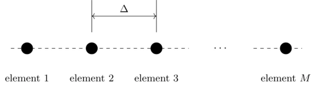
which means that the conjugate ofAflipped over the horizontal axis is the same asA. The uniform linear array (ULA) is an example of an array whose steering matrix is left centro-hermitian. As can be seen in Figure 2.5, the ULA has M equally-spaced elements arranged in a linear fashion with spacing∆.
· · ·
element 1 element 2 element 3 element M
∆
Figure 2.5: Uniform Linear Array with∆spacing
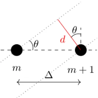
As can be seen in Figure 2.6, for adjacent elementsm and m+ 1 spaced ∆apart, the wavefront coming at an angleθwill pass the first element and then the next after traveling a
distance ofd:
m m+ 1
∆ d
θ
θ
Figure 2.6: Wavefront incidence on adjacent array elements
Since the spacing is known, the distance traveled by the wavefront isd= ∆ sinθand the travel time between each element can be calculated as
τ = d
c =
∆ sinθ
c . (2.53)
A narrowband signal sm(t) = ej2πf t at the m-th element will arrive at the m + 1-th
element with a delayτ and will be
sm+1(t) =ej2πf(t+τ)
=ej2πf tej2πf τ
=ej2πf tejµ. (2.54)
withµdenominated the spatial frequency and is
µ= 2πf τ
= 2πf∆ sinθ
c . (2.55)
Since the structure of the array is uniform, the signal at each subsequent element in the array is shifted by exactly ejµ. Arranging the signal received at allM elements into a vector
s(t)∈CM
s(t) =
ej2πf t
ej2πf tejµ
.. .
ej2πf tej(M−2)µ
ej2πf tej(M−1)µ
=ej2πf t
1 ejµ .. .
ej(M−2µ
ej(M−1)µ
=ej2πf ta(µ). (2.56)
in whicha(µ)∈CM is known as the steering vector and eachm-th element is ej(m−1)µ. This
is known as the Vandermonde structure.
To make the Vandermonde structure steering vectora(µ)conform to the condition set in (2.51), it has to be multiplied by e−jM−1
2 µfor evenM or e−j⌊
M
2⌋µfor oddM, and it becomes
a(µ) evenM =
e−jM−1
2 µ
e−jM−2
2 µ
.. .
e−j1 2µ
ej1 2µ
.. .
ejM−2
2 µ
ejM−1
2 µ
a(µ) oddM =
e−j⌊M
2 ⌋µ
e−j⌊M−2 2 ⌋µ
.. .
1
.. .
ej⌊M−2
2 ⌋µ
ej⌊M2⌋µ
. (2.57)
For L sources impinging on the array the contribution of each a(µl), l = 1, . . . , L is
concatenated into a steering matrixA= [a(µ1), . . . ,a(µL)]∈CM×L:
A evenM =
e−jM−1
2 µ1 · · · e−j
M−1 2 µL
e−jM−2
2 µ1 · · · e−j
M−2 2 µL
..
. ... ...
e−j1
2µ1 ... e−j 1 2µL
ej1
2µ1 ... ej 1 2µL
..
. ... ...
ejM−2
2 µ1 · · · ej
M−2
2 µL
ejM−1
2 µ1 · · · ej
M−1
2 µL
A oddM =
e−j⌊M−1
2 ⌋µ1 · · · e−j⌊
M
2 ⌋µL
e−j⌊M−2
2 ⌋µ1 · · · e−j⌊
M−2 2 ⌋µL
..
. ... ...
1 ... 1
..
. ... ...
ej⌊M−2
2 ⌋µ1 · · · ej⌊
M−2 2 ⌋µL
ej⌊M−1
2 ⌋µ1 · · · ej⌊
M
2 ⌋µL
, (2.58)
and (2.51) holds.
For a ULA with half-wavelength spacing∆ =λ/2the spatial frequency is
µ= 2πf(λ/2) sinθ c
=πsinθ. (2.59)
Chapter 3
Tensor-based Approaches to Time-Delay
Estimation
In this chapter, three algorithms are presented. The state-of-the-art tensor-based time-delay estimation from [5], and two novel approaches for filtering and time-time-delay estima-tion. The first approach is based on closed DoA estimation of the steering factor matrix followed by a simultaneous estimation of the complex amplitude and code factor matrices using Khatri-Rao factorization. The second approach uses an iterative least-squares ortho-gonal Procrustes problem (OPP) and Khatri-Rao factorization to estimate the steering and complex amplitude factor matrices.
3.1 State-of-the-Art Tensor-Based Time-Delay Estimation
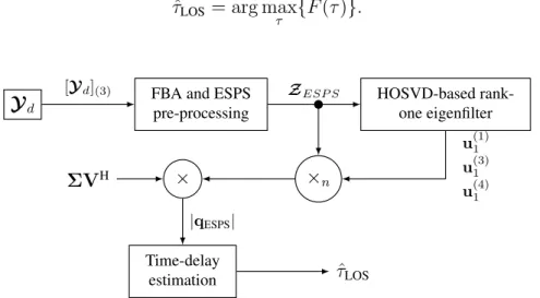
In this section, we summarize the state-of-the-art tensor-based time-delay estimation ap-proach, which is an HOSVD based eigenfilter with Forward Backward Averaging (FBA) and Expanded Spatial Smoothing (ESPS).
This chapter is divided into three sections which are also the steps of the state-of-the-art approach according to Figure 3.1. First a pre-processing step is applied to incorporate FBA and ESPS as illustrated in Figure 3.1 and detailed in Section 3.1.1. Next the HOSVD based rank-one filters are computed for three dimensions of the tensor and an improved output of the correlator bank is obtained as shown in Figure 3.1 and also according to Section 2.3.5. Finally, the amount of points is increased via a cubic spline interpolation and one dimension peak search is performed in order to locate the time-delay of the multidimensionally filtered output as presented in Section 3.1.3.
3.1.1 Forward-Backward Averaging and Expanded Spatial Smoothing
Similarly to matrix-based FBA [16], flipped identity matrices are used to duplicate the number of samples. The left-hand multiplication matrixΠM ∈ RM×M is an identity matrix
of size M flipped along its vertical axis and the right-hand multiplication matrixΠKQ ∈ RKQ×KQ likewise. These matrices are applied to the spatial (third-mode) unfolding of the
signal tensor in the following manner:
Z=h[Yd](3) ΠM[Yd]∗(3)ΠKQ
i
∈CM×2KQ. (3.1)
In a similar fashion to matrix-based SPS [18], selection matrices that divide the array into
LS subarrays withMS =M−LS+ 1elements are used. The selection matrices are defined
as
JlS =
h
0MS×lS−1 IMS 0MS×LS−lS
i
∈RMS×M, (3.2)
forlS = 1, . . . , LS.
Using the selection matrices, spatial smoothing is applied to the forward-backward ave-raged spatial unfolding of the signal tensor
W=hJ1Z · · · JLSZ
i
∈CMS×2LSKQ, (3.3)
and W is third-mode folded back into a forward-backward averaged spatially-smoothed fourth-order tensorZESPS ∈C2K×Q×MS×LS.
3.1.2 Higher-Order SVD eigenfiltering
For time-delay estimation the HOSVD is applied toZESPS
ZESPS =R×1U(1)×2U(2)×3U(3)×4U(4), (3.4)
in which R ∈ C2K×Q×MS×LS is the core tensor, and U(1) ∈ C2K×2K, U(2) ∈ CQ×Q,
U(3) ∈ CMS×MS, and U(4) ∈ CLS×LS are unitary matrices collecting singular vectors of
each mode’s respective unfolding [15].
By assuming the LOS signal component has the greatest power compared with NLOS signal components, the dominant singular vectors of the first, third and fourth dimensions of ZESPS in (3.4) are mostly correlated to the LOS signal component. Therefore, [5] has proposed the following HOSVD based eigenfilter:
qESPS =
ZESPS×1(u(1)1 )
H
×3(u(3)1 )
H
×4(u(4)1 )
H
Note thatΣVHis computed in (2.47).
3.1.3 Time-Delay Estimation
In order to obtain the time-delay estimation fromqESPS, a cubic spline interpolation based on |qESPS|is used to generate a cost functionF(τ). The τ variable that maximizes the cost function is computed as follows
ˆ
τLOS = arg max
τ {F(τ)}. (3.6)
Yd
FBA and ESPS pre-processing
HOSVD-based rank-one eigenfilter
×n
× ΣVH
Time-delay
estimation τˆLOS
[Yd](3) ZESP S
u(1)1 u(3)1 u(4)1
|qESPS|
Figure 3.1: Block diagram of the state-of-the-art HOSVD eigenfilter-based time-delay esti-mation approach
3.2 Proposed DoA Estimation and KRF Approach
In this chapter, we propose a three step approach based on the direction of arrival (DoA) estimation, the Khatri-Rao factorization (KRF) and the selection of the estimated LOS time-delay. Note that to estimate the DoA of the LOS and NLOS signal components, the model order Ld should be known. Therefore, we refer to the tensor based model order selection
schemes in [25, 26, 27].
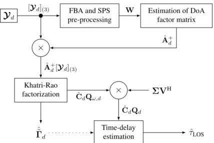
This section is divided into three subsections. After a pre-processing step via FBA and ESPS is applied as illustrated in Figure 3.2, DoA estimation is utilized to rebuild the fac-tor matrix A as described in Subsection 3.2.1. Then Khatri-Rao factorization is applied to the product of Aˆ+
d and[Yd](3) to estimate the factor matricesΓˆ˜dand CˆdQω,d according to
Subsection 3.2.2. Finally, the LOS signal component of the estimated signal is found the time-delay is estimated as described in Subsection 3.2.3.
3.2.1 Estimation of DoA factor matrix
Since Qω,d has been applied to the received signals as shown in (2.48), there are only
Ld signal components and we desire to estimate the DoA of all Ld components. Note that
ˆ
Ld can be estimated by using the tensor based model order selection schemes discussed
in [25, 26, 27].
As shown in Figure 3.2, DoA estimation is applied to the forward-backward averaged spatially smoothed signal matrixWcalculated in (3.3).
Although there are several DoA schemes in the literature, due to the simplicity, good ac-curacy and low computational complexity, we use in our work the Estimation of Signal Para-meter via Rotational Invariance Technique (ESPRIT) [28]. We assume the GNSS receiver is equipped with an antenna array, whose geometry is Vandermonde and left centro-hermitian.
3.2.2 PR code and complex amplitude estimation via Khatri-Rao
Fac-torization
By rewriting the spatial unfolding of the noiseless signal from (2.50), the following ex-pression is obtained:
[Y0,d](3) =Ad
˜
ΓTd⋄(CdQω,d)T
T
∈CM×KQ. (3.7)
OnceAˆdhas been estimated, its pseudo-inverse can be applied to (3.7) such that ˆ
A+d[Y0,d](3) = ˆA+dAd
˜
ΓTd⋄(CdQω,d)T
T
≈Γ˜Td ⋄(CdQω,d)T
T
∈CLd×KQ, (3.8)
and the factor matricesΓ˜dandCdQω,d can be estimated by Least Squares Khatri-Rao facto-rization (LSKRF) [29].
Given(˜ΓTd⋄(CdQω,d)T), and considering it’sld-th column can be calculated as the
Khatri-Rao product of theld-th column ofΓ˜Tdand(CdQω,d)T:
˜
ΓTd⋄(CdQω,d)T
·,ld
= (˜ΓTd)·,ld⋄(CdQω,d)
T
·,ld, (3.9)
with each column(˜ΓTd⋄(CdQω,d)T)·,ld ∈C
KQ.
To solve for estimates ofΓ˜dandCdQω,d, we reshape (3.9) into a matrix of sizeQ×K: unvec
Q×K
˜
ΓTd⋄(CdQω,d)T
·,ld
= (CdQω,d)T·,ld(˜Γ
T
d)
T
Since (3.10) is a rank-one matrix, we can use a SVD-based rank-one approximation:
unvec
Q×K
˜
ΓTd⋄(CdQω,d)T
·ld
=UldΣldVld. (3.11)
The estimates for(˜ΓTd)·,ld and ((CdQω,d)
T)
·,ld are
√σ
ld,1v
∗
ld,1 and
√σ
ld,1uld,1,
respecti-vely, where σld,1 is the dominant singular value of Σld, uld,1 is the dominant left singular
vector ofUld, andv
∗
ld,1 is the conjugate of the dominant right singular vector ofVld. This is
repeated forld = 1, . . . , Ld.
OnceCˆdQω,d is estimated using LSKRF, the next step is to find which row corresponds to the LOS signal component due to possible permutation ambiguities in Aˆd estimated in 3.2.1.
3.2.3 LOS Time-Delay Estimation
In order to find the time-delay of the LOS signal component, two schemes are proposed, namely, greatest power based scheme and smallest delay based scheme.
For the greatest power based scheme, we assume that the LOS signal component is not blocked. Therefore, the LOS signal component has the greatest power in comparison with the multipath components. In this case, the following expression can be used to locate the estimated LOS signal component,ˆcLOS:
lLOS= max
ld k
ˆ˜
Γd,ld·k2, (3.12)
in whichΓˆ˜d,ld·is theld-th row of the matrixΓˆ˜d. Note that in the greatest power based scheme,
we just compute the delay of the selected component using the following expression
qDoA/KRF= ˆcTLOSQω,dΣVH, (3.13)
followed by a cubic spline interpolation to obtain a cost function and estimate the time-delay as in (3.6).
For the smallest time-delay based scheme, we compute the Ld time-delays of ˆcld for
ld = 1, . . . , Ld. Using the resulting time-delay estimation vectorτˆ = [ˆτ1, . . . ,τˆLd]
T ∈ RLd,
the LOS time-delay is found by solving
ˆ
τLOS = min
τ {τˆ}. (3.14)
Yd
FBA and SPS pre-processing
Estimation of DoA factor matrix
×
Khatri-Rao
factorization × ΣVH
ˆ˜ Γd
Time-delay
estimation τˆLOS
[Yd](3) W
ˆ
A+d
ˆ
A+d[Yd](3)
ˆ
CdQω,d
ˆ
CdQd
Figure 3.2: Block Diagram of the proposed DoA/KRF time-delay estimation approach
3.3 Procrustes estimation and Khatri-Rao factorization
(ProKRaft) filtering
In this section we present an iterative approach based on the Orthogonal Procrustes Pro-blem (OPP) and KRF to calculate the DoA and complex amplitude factor matrices simulta-neously. Since this technique relies on separating the subspace of the SVD, the model order
Ldshould be known.
3.3.1 Simultaneous DoA and amplitude factor matrix estimation
To simultaneously estimate the factor matricesAdandΓd, the ProKRaft approach relies
on the fact that a Hermitian unfolding can be achieved by calculating the multimode covari-ance matrix, Rmm, which is the product of the transpose and conjugate of the second-mode unfolding ofYddivided by the number of samples,N,
Rmm = [Yd]T(2)[Yd]∗(2)/N (3.15)
= (Ad⋄Γ˜Td) (CdQω,d)(CdQω,d)H/N
| {z }
RC
(Ad⋄Γ˜Td)
H (3.16)
= (Ad⋄Γ˜Td)RC(Ad⋄Γ˜Td)
H
∈CM K×M K, (3.17)
in whichRC ∈ RLd×Ld is the covariance matrix of the LOS and NLOS signal components
from satellited.
ConsideringRC≈ILd, the multimode covariance matrix can be approximated as
Rmm≈(Ad⋄Γ˜dT)(Ad⋄Γ˜Td)
H
, (3.18)