ANÁLISE DE UM AMORTECEDOR DE COLUNA
DE LÍQUIDO SINTONIZADO EM UMA TURBINA
EÓLICA SUJEITA A CARREGAMENTO
ALEATÓRIO
Por,
Mansour Hassan Alkmim
DISSERTAÇÃO DE MESTRADO EM CIÊNCIAS MECÂNICAS
UNIVERSIDADE DE BRASÍLIA
FACULDADE DE TECNOLOGIA
UNIVERSIDADE DE BRASÍLIA FACULDADE DE TECNOLOGIA
DEPARTAMENTO DE ENGENHARIA MECÂNICA
ANÁLISE DE UM AMORTECEDOR DE COLUNA
DE LÍQUIDO SINTONIZADO EM UMA TURBINA
EÓLICA SUJEITA A CARREGAMENTO
ALEATÓRIO
MANSOUR HASSAN ALKMIM
ORIENTADOR: ADRIANO TODOROVIC FABRO
DISSERTAÇÃO DE MESTRADO EM CIÊNCIAS MECÂNICAS PUBLICAÇÃO: ENM.DM
UNIVERSIDADE DE BRASÍLIA FACULDADE DE TECNOLOGIA
DEPARTAMENTO DE ENGENHARIA MECÂNICA
ANÁLISE DE UM AMORTECEDOR DE COLUNA DE
LÍQUIDO SINTONIZADO EM UMA TURBINA EÓLICA
SUJEITA A CARREGAMENTO ALEATÓRIO
MANSOUR HASSAN ALKMIM
DISSERTAÇÃO DE MESTRADO SUBMETIDA AO DEPARTAMENTO DE ENGENHARIA MECÂNICA DA FACULDADE DE TECNOLOGIA DA UNIVERSIDADE DE BRASÍLIA, COMO PARTE DOS REQUISITOS NECESSÁRIOS PARA A OBTENÇÃO DO GRAU DE MESTRE EM CIÊNCIAS MECÂNICAS.
APROVADO POR:
Adriano Todorovic Fabro DSc. (ENM/ UnB) (Orientador)
Aline Souza de Paula DSc. (ENM/ UnB) (Examinadora interna)
Sergio Henrique da Silva Carneiro DSc. (FGA/ UnB) (Examinador externo)
Acknowledgments
I would like to express my sincere appreciation and respect to my supervisors DSc. Adriano T. Fabro and DSc. Marcus V. G. de Morais for their guidance, advise and encouragement in carrying out this research. A especial thanks to DSc. Aline S. de Paula for the opportunities that opened many doors for me during graduation.
I also would like to thanks my colleagues from the Dynamic System’s Group with whom I shared my time at University of Brasilia.
Finally, a especial note of gratitude goes to my family for their moral and financial support through out my life.
We know the past but cannot control it. We control the future but cannot know it.
Resumo
Os sistemas passivos de dissipação de energia abrangem uma variedade de materiais e dispositivos para melhorar o amortecimento de estruturas. Entre os atuais sistemas de dissipação de energia passiva, o amortecedor de coluna de líquido sintonizado (TLCD), uma classe de controle passivo que utiliza líquido em um reservatório de forma “U”, tem sido amplamente pesquisado em diversas aplicações. O principal objetivo desta dissertação é desenvolver técnicas de análise numéricas e experimentais para um TLCD com aplicação em turbinas eólicas submetido a cargas de vento aleatório.
A análise numérica está dividida em duas etapas. A primeira etapa considera o modelo determinístico da turbina e TLCD. Um algoritmo de otimização é utilizado para encontrar parâmetros ótimos do TLCD submetido a espectros de vento aleatório. Em seguida, um exemplo numérico com um modelo de turbina eólica simplificado é estudado para ilustrar a eficácia do TLCD e é mostrado que diferentes espectros de vento podem afetar significativamente os resultados de otimização, isto é, os parâmetros do TLCD. Os resultados no tempo e frequência da análise de vibração aleatória mostram uma redução satisfatória dos níveis de vibração de resposta.
Na segunda etapa, considera-se o modelo não determinista com objetivo de quantifi-car incertezas nos parâmetros do TLCD e da estrutura. A função de resposta em frequência do sistema com TLCD é investigada considerando dois casos de incerteza de parâmetros. Para o primeiro caso, os resultados mostraram que a incerteza só é predominante perto da região de ressonância e antirressonância e pode interferir na condição ideal do TLCD. Para o segundo caso, as incertezas estão presentes em todas a faixa de frequência.
Finalmente, uma análise experimental é realizada. A caracterização dos parâmetros modais do TLCD e da estrutura é realizada e os resultados numéricos e teóricos se mostram em boa concordância. Em seguida, A resposta do sistema acoplado é investigada. Os resultados mostram que o efeito da massa adicional é o predominante. Embora o efeito do TLCD tenha sido pequeno, ele apresenta uma redução de vibração próximo a sua frequência natural.
Palavras-chaves: vibração aleatória, análise estocástica, otimização, quantificação
Abstract
Passive energy dissipation systems encompass a range of materials and devices for enhancing damping. Among the current passive energy dissipation systems, tuned liquid column damper (TLCD), a class of passive control that utilizes liquid in a “U” shape reservoir to control structural vibration of the primary system, has been widely researched in a variety of applications. The main objective of this thesis is to develop numerical and experimental analysis techniques for a liquid column damper subjected to random wind loads with particular application in wind turbines.
The numerical analysis in this thesis is divided in two stages. The first stage consider the deterministic model of the wind turbine and TLCD. An optimization approach is used to search for optimized parameters considering different wind spectrums. Then, a numerical example with a simplified wind turbine model is given to illustrate the efficacy of TLCD and it is shown that different wind spectra can significantly affect the optimization results, i.e. the TLCD parameters. Time and frequency domain results from the random vibration analysis are shown with satisfactory reduction of the response vibration levels. In the second stage, nondeterministic model is studied with goal to quantify uncertainties in the damper and structure parameters. The frequency response function is investigated considering two cases of parameter uncertainty. The results showed that, for the former, the uncertainty is only predominant near the resonance and anti-resonance region and can indeed interfere in the optimum condition of the absorber. For the latter, the uncertainties are presented in frequency range.
Finally, an experimental characterization of the TLCD and structure is carried out. The characterization of the modal parameters of the TLCD and the structure is performed and the numerical and theoretical results that show good agreement. Then, the response of the coupled system is investigated. Results showed that the effect of added mass is predominant. While the effects of TLCD were minimal, it showed a vibration reduction which validated the correctly tuned TLCD near its natural frequency.
Key-words: random vibration, stochastic analysis, optimization, uncertainty
Contents
1 INTRODUCTION . . . . 1
1.1 The objectives of the study . . . . 2
1.2 Organization of the Thesis . . . . 3
2 STRUCTURAL CONTROL . . . . 5
2.1 Introduction . . . . 5
2.2 Passive control . . . . 7
2.2.1 Tuned mass damper (TMD) . . . 8
2.2.2 Tuned liquid damper (TLD) . . . 9
2.3 Previous works . . . 11
3 FUNDAMENTALS OF RANDOM VIBRATION . . . 15
3.1 Random vibration . . . 15
3.2 Probability density function . . . 17
3.3 Stochastic process . . . 18
3.4 Correlation and autocorrelation . . . 19
3.5 Fourier series and the Fourier transform pair . . . 20
3.5.1 The complex form of the Fourier series . . . 21
3.5.2 Fourier integrals . . . 22
3.5.3 Discrete Fourier transform . . . 23
3.5.4 Fast Fourier transform . . . 24
3.6 Spectral analysis . . . 26
4 PROBABILIST DESCRIPTION OF WIND LOADS . . . 29
4.1 The wind behavior near ground . . . 29
4.2 Short-term wind model . . . 31
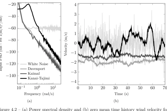
4.3 Wind profile power spectral density . . . 33
5 MATHEMATICAL DESCRIPTION OF DYNAMIC SYSTEM . 36 5.1 Equivalent parameters of a cantilever beam . . . 38
6 OPTIMIZATION . . . 44
6.1 Parameter optimization criteria . . . 45
6.1.1 Generalized patter search . . . 47
6.1.2 Verification procedure . . . 47
6.2 Random vibration analysis . . . 49
6.2.1 Numerical example . . . 50
6.3 Concluding remarks . . . 52
7 UNCERTAINTY ANALYSIS . . . 55
7.1 Uncertainty model . . . 56
7.2 Monte Carlo sampling . . . 58
7.3 Results for parameter uncertainty . . . 59
7.4 Concluding remarks . . . 62
8 EXPERIMENTAL ANALYSIS . . . 63
8.1 Identification of modal data . . . 63
8.2 Experimental setup . . . 68
8.2.1 Structure characterization . . . 69
8.2.2 TLCD characterization . . . 72
8.3 Structural dynamic response with a TLCD . . . 74
8.3.1 Experiment 1: root mean square method . . . 75
8.3.2 Experiment 2: structure free response . . . 76
8.4 Concluding remarks . . . 79 9 FINAL REMARKS . . . 81 9.1 Future works . . . 83 9.2 List of publications . . . 83 REFERENCES . . . 85
APPENDIX
90
List of Figures
Figura 2.1 – Diagram of an active control system (Constantinou et al., 1998). . . 7
Figura 2.2 – Diagram of a passive control system (Constantinou et al., 1998). . . 8
Figura 2.3 – Example of a TMD, undamped system with main mass subjected to harmonic excitation (Soong & Dargush, 1997). . . 10
Figura 2.4 – Example of a TLCD in a wind turbine (Altay et al., 2014). . . 14
Figura 3.1 – A sample of a non-deterministic signal . . . 17
Figura 3.2 – Normal, or Gaussian probability density function . . . 18
Figura 3.3 – Random samples of a process . . . 19
Figura 3.4 – Fourier expansion of a square wave periodic signal with partial sums of the 𝑛 = 1, 𝑛 = 3 and 𝑛 = 20 terms of the expansion. . . . 21
Figura 3.5 – Four Fourier representation of signals . . . 24
Figura 4.1 – Typical power spectrum of the horizontal velocity of wind at 100 m above the ground. . . 30
Figura 4.2 – (a) Power spectral density and (b) zero mean time history wind velocity for white noise, Davenport, Kaimal and Kanai-Tajimi models. . . 34
Figura 5.1 – Diagram of a completed model of forces acting on a wind turbine (Ageze et al., 2017). . . 37
Figura 5.2 – Schematic model of the structure and equivalent simplified model. . . . 39
Figura 5.3 – The (a) first and (b) second modes of vibration of a cantilever beam with tip mass (Hatch, 2000). . . 40
Figura 5.4 – Schematic model of the TLCD. . . 42
Figura 6.1 – Comparing optimized (a) tunning ratio and (b) damping ratio subject to White Noise spectrum as a function of the mass ratio 𝜇 for different length ratio 𝛼. . . . 48
Figura 6.2 – Response PSD 𝑆𝑦𝑦(𝜔) obtained from frequency response function for the linearized case (upper path), and from numerical integration for the nonlinear case (lower path). . . 49
Figura 6.3 – PSD response of main system to a first order filter random excitation without and with TLCD, obtained via statistical linearization and via numerical integration of nonlinear system . . . 50
Figura 6.4 – Optimum (a) tunning ratio 𝛾𝑜𝑝𝑡 and (b) damping ratio 𝜁𝑜𝑝𝑡 subject to
different wind spectra as a function of the mass ratio 𝜇 for a fixed length ratio 𝛼 = 0.8 and 1% primary structural damping. . . . 52 Figura 6.5 – Response of main system under Kaimal spectrum for 𝜇 = 0.06 and
𝛼 = 0.8 (a) without TLCD (dashed), optimized (solid black) and two
different mass ratio (solid grey scale) in the frequency domain and (b) without TLCD (solid grey scale) and optimized (solid black) in the time domain. . . 53 Figura 7.1 – FRFs amplitude with TLCD damping ratio uncertainties showing the
deterministic model response, mean response of the stochastic model, and 95% confidence region for different values of 𝛿𝑍’s: (a) .2 (b) .4 (c)
.6 (d) .7. . . 60 Figura 7.2 – FRFs amplitude with TLCD damping ratio and structure stiffness
uncertainties showing the deterministic model response, mean response of the stochastic model, and 95% confidence region for different values of 𝛿𝑍 and 𝛿𝐾: (a) .2 & .05 (b) .4 & .15 (c) .6 & .25 (d) .7 & .35. . . 61
Figura 7.3 – Mean square convergence for (a) variability in 𝛿𝑍 and (b) variability in
both 𝛿𝑍 and 𝛿𝐾. . . 62
Figura 8.1 – Nyquist circle showing relevant angles for modal analysis. . . 67 Figura 8.2 – Experimental structure assembly showing the main structural components. 69 Figura 8.3 – Schematic representation of experimental procedure to characterize the
structure. . . 70 Figura 8.4 – Estimated FRF 𝐻1 for different masses (black: 𝑚 = 0 kg, red: 𝑚 = 2
kg, blue: 𝑚 = 5 kg, purple: 𝑚 = 7 kg). . . . 71 Figura 8.5 – Experimental and theoretical first mode natural frequency 𝑓𝑛,𝑒 with
respect to tower length 𝐿 for different masses. . . . 72 Figura 8.6 – Schematic representation of TLCD experimental procedure. . . 73 Figura 8.7 – Float fish bait used for capture the vertical displacement of the liquid
column. . . 73 Figura 8.8 – Fitted curve of rectangular tlcd vertical displacement with respect to
time and fitted coefficients. . . 73 Figura 8.9 – Diagram for the inverse approach for the testing procedure. An iterative
process is used to determine the optimized structure length based on the TLCD’s geometry. . . 75 Figura 8.10–Experimental input (gray) and output (black) normalized sinusoidal
functions. . . 76 Figura 8.11–Experimental data for the RMS ratio between the output and input
signal from three configurations, 𝑚𝑎𝑑𝑑= 6 kg, 𝑚𝑎𝑑𝑑= 5 kg with TLCD,
𝑚𝑎𝑑𝑑= 3 kg with TLCD. . . 77
Figura 8.12–Experimental structure with and without TLCD for tracking the struc-ture displacement. . . 77
Figura 8.13–Experimental (a) displacement and (b) output PSD of structure with length 𝐿 = 0.98 m for the case without TLCD with added mass 𝑚𝑎𝑑𝑑=
8.4 kg and configuration using a TLCD (1.1 kg) with added mass
𝑚𝑎𝑑𝑑= 7.3. . . . 78
Figura 8.14–Output PSD of structure with length 𝐿 = 0.98 m for the case without TLCD with added mass 𝑚𝑎𝑑𝑑 = 10 kg and configuration using a TLCD
List of Tables
Tabela 2.1 – Summary of classification of passive control systems and common passive
control devices . . . 9
Tabela 4.1 – Roughness class of different site types . . . 32
Tabela 4.2 – Common power spectral density functions models. . . 34
Tabela 6.1 – Wind turbine parameters . . . 51
Tabela 6.2 – Optimized LCD damping ratio 𝜁𝑜𝑝𝑡 and tunning ratio 𝛾𝑜𝑝𝑡 for a fixed length ratio 𝛼 = 0.8 and 1% primary structural damping . . . . 52
Tabela 8.1 – Structure masses and moment of inertia . . . 70
List of Simbols
𝐻 Frequency response function
ℎ Impulse response function
𝑗 Imaginary number 𝑡 Time [s] 𝜔 Frequency [rad/s] 𝑓 Frequency [Hz] 𝑇 Period [s−1] 𝜏 Time interval [s]
Δ Sampling time interval [s]
𝑃 Probability distribution function
𝑝 Probability density function
𝑥 Input function in time domain (Chapter 3)
𝑥 Displacement of the structure (Chapter 5)
𝑦 Output function in time domain
𝐸 Expected value 𝐸[𝑥]
𝑅 Correlation function 𝑅(𝜏 )
𝑆 Spectral density 𝑆(𝜔)
𝑣 mean wind velocity
𝑧0 hub height
𝜌𝑎𝑖𝑟 air density
𝛽 roughness coefficient
𝑐 Weibull mode parameter
𝜓 Turbulence intensity
𝑣ℎ𝑢𝑏 Mean value of the hub height velocity
𝑤 Transverse displacement response
𝑐 Weibull mode parameter
𝜑 Spatial displacement
𝑌 Temporal displacement
𝐸 Elastic modulus
𝐿 Tower length
𝐼 Moment of inertia
𝐽 Rotary mass moment of inertia
𝑀 Cantilever beam tip mass
𝑚 Cantilever beam distributed mass
𝐷 Cantilever beam width
𝑡ℎ Cantilever beam thickness
𝐴ℎ Cantilever beam cross section
𝜌𝑠 Steel density
𝜆 Roots of the eigenvalue problem
𝜔𝑛 Natural frequency cantilever beam
𝑇 Kinetic energy
𝑀* Generalized mass
𝑉 Potential (strain) energy
𝐾* Generalized stiffness
𝑢 Displacement of fluid
𝜌 Water density
𝐴 Cross section area of TLCD 𝑏 Horizontal length of TLCD 𝑙 Total length of TLCD 𝑔 Gravity constant 𝑚𝑎 Mass of TLCD 𝑐𝑎 damping of TLCD 𝑘𝑎 stiffness of TLCD 𝜔𝑎 Natural frequency of TLCD 𝜁𝑎 Damping ratio of TLCD 𝑚𝑒 Mass of structure 𝑐𝑒 damping of structure 𝑘𝑒 stiffness of structure
𝜔𝑒 Natural frequency of structure
𝜁𝑒 Damping ratio of structure
𝐹 Excitations force
𝛼 Length ratio
𝜇 Mass ratio
𝛾 Tuning ratio
Ξ performance index (cost function)
𝜔𝑒 Natural frequency of structure
Φ Mass normalized mode shape (eigenvectors) Ψ General normalization mode shape (eigenvectors)
1 Introduction
The current Brazilian energy scenario is undergoing impactful changes. There is a clear need to adjust the current energy sector that presents an imbalance. Brazil depends almost exclusively on hydroelectric power. According to data released by PNE 2030 (National Energy Plan), most of the energy produced in the country comes from hydroelectric plants. By the year 2030, it is expected that hydroelectric plants will have a share of 77.4 % of the energy matrix (Pottmaier et al., 2013).
Despite all the benefits of the hydroelectric plants, there are uncertainties about their future supply. Major projects such as S. Luiz do Tapajós and Belo Monte have faced serious socio-environmental conflicts such as the transposition of rivers, impacts on the fauna and conflicts with local communities. Another critical aspect of hydroelectric plants is the existence of a great dependence on the climatic conditions and the location of this energy, found primarily in the Amazon region. Moreover, recent examples of poor management of water levels in reservoirs led to the reactivation of thermoelectric plants that generate environmental and economic damages.
Since there is a need to diversify the Brazilian energy matrix, other energy sources that are efficient and renewable are sought. Among the possible options that stand out, wind and solar energy are becoming good options due to good geographical and economic conditions (Jong et al., 2013).
The increasing height of wind turbine increases the need of new methods to ensure structural reliability. Wind turbines are structures that convert the mechanical movement generated by the force of the winds into electric energy. The wind reaches the rotor blades that transfer the rotational motion to an electric generator responsible for producing electricity.
During the design phase, wind turbines must meet a wind speed that produces the maximum output power. Occasionally, the wind forces can be dangerously high which forces the control system to limit the movement of the blades in order to avoid overloading of the rotor, the gearbox and the generator. Usually, wind turbines have angular control systems in the turbines and brakes that maintain integrity and prevent excessive vibration of the towers. These systems are useful because they regulate rotor speed based on wind speed under certain operating conditions. Generally, wind turbines have small damping values compared to other structures. The damping ratio resulting from aerodynamic
damping corresponds to 1-2 % (Altay et al., 2014).
Concerns over the integrity of wind turbines throughout the years have become a key point during design phase. The advance of the technology in wind turbines have caused an increase in its size and efficiency. In this way, challenges arise to avoid excessive vibration of both propellers and towers. Higher and more slender structures also raise concerns over their integrity and longevity.
The dynamic behavior of wind turbines has led to several technical studies in recent years. The reduction of vibration, with the purpose of increasing its lifespan, motivates the use of several passive or semi-active vibration control techniques. Among the various vibration control proposals, tuned liquid column dampers (TLCDs) have been considered in several publications in recent years and have become a feasible option with relative low cost and good efficiency.
Analyzing the dynamic response in the frequency domain has proven to be a feasible initial approach of understanding the wind turbine behavior. Design optimization can be carried out rapidly in the frequency domain to increase the damper efficiency. A more rigorous analysis can be carried out after the initial parameter optimization in the frequency domain is completed. This approach increase qualitative and quantitative understanding and can lead to reduced design costs and better optimized schemes.
Some of the questions we hope to address in this thesis are:
∙ To what extent will the vibration suppression take place with the added damper? ∙ Is the simplified model of wind turbine acceptable? Why?
∙ How much can the vibration suppression be improved from optimized parameters? ∙ How much variability the TLCD’s parameters have? How does it influence the turbine
performance?
∙ How the model and dynamic response of the structure compare with experimental data?
1.1
The objectives of the study
The main objective of the study is to develop numerical and experimental techniques to investigate the behavior of a liquid column damper subjected to random wind loads with particular application in wind turbines. For this reason, we have the following secondary objectives:
∙ a numerical analysis considering the deterministic model of the wind turbine and TLCD with goal of controlling the structure for small displacement without
consi-dering the rotational inertia from the blades. An optimization approach is adopted which allows the search of optimized parameter considering different wind spectrums. ∙ a numerical analysis considering the nondeterministic model with goal of quantifying
uncertainties in the TLCD’s damper and structure stiffness.
∙ an experimental phase is carried out with goal of characterization of the TLCD and structure and then compare it with numerical result.
1.2
Organization of the Thesis
This thesis is organized as follows.
Chapter 1 presents the introduction and objectives.
Chapter 2 presents some of the main structural control techniques in suppressing vibration of structures. First, the state of the art of structural control is presented. Then, the relevant types of control systems are discussed. Emphasis will be given to passive controls and more specifically on the tuned liquid absorbers and their use in wind turbines which is the subject of this work. A literature review is presented considering the use of absorbers in several applications and their development in recent years.
Chapter 3 presents a review on fundamental concepts of random vibration and probability theory. The aim is to review the key principles of the probability theory and thus facilitate its application to solve problems in random vibration.
Chapter 4 deals with the effects of the probabilistic aspect of wind in low atmospheric layers on flexible structures. The problems is confined to along-wind response of structures. Moreover, cross-wind response or aero-elastic coupled problems are left out of discussion. The idea is to discuss some general notions, which should cast some light on the complexity of the phenomenon.
Chapter 5 discusses how winds influence the dynamic behavior of the structure and how to optimize the TLCD with respect to different wind spectrums. It is therefore of interest to study how a simplified dynamic model could estimate the structural response. The simplified model has to be reduced to the elementary coordinates but still have to describe the relevant physical process under consideration with good accuracy. Such a simplified model can be used as an early design of new wind turbines. This work focus on the structural dynamic aspect of structures such as lattice towers with concentrated mass at the top, hence, the model does not include the gyroscopic effects due to turbine blade rotation.
In Chapter 6 we propose the use of a optimization algorithm for the TLCD’s parameters subjected to an arbitrary wind spectra, given by its power spectral density (PSD). A simple verification is made considering the analytical solution of undamped
primary structure under white noise excitation. Finally, a numerical example with a simplified wind turbine model is given to illustrate the efficacy of TLCD. Time and frequency domain results from the random vibration analysis are also shown.
In Chapter 7, parametric uncertainties in a TLCD applied in wind turbines are investigated. The assumption that uncertainties in structures have negligible response can be unacceptable in real situations and, beside that, uncertainties in the performance-related cannot be included in the damper parameter optimization. For this reason, to increase the credibility of the model, these uncertainties are included to help describe the range of potential outputs of the system at some probability level and estimate the relative impacts of input variable uncertainties. Two different cases are studied, the first one we only consider uncertainties in the absorber damping ratio and, in the second case, we consider both uncertainties in the absorber damping ratio and the structural stiffness.
Finally, in Chapter 8, an experimental setup built in the Vibration Laboratory of the Dynamic Systems Group (GDS) is proposed. An experimental procedure is carried out to characterize the modal parameters of the TLCD and structure. Finally, the response of the coupled system is investigated.
2 Structural Control
Structural control can be an important part of designing new structure and retrofit-ting exisretrofit-ting ones. Design for strength alone does not necessarily ensure that the structure will respond well dynamically. It was during the Second World War that concepts such as vibration isolation, vibration absorption and vibration damping were developed and effec-tively applied to aircraft structures. The technology quickly moved into civil engineering. Similar to the general controls literature, the structure control tends to represent diverse interests and viewpoints, though all share common goal: the protection of buildings and the people around them.
This chapter presents some of the main structural control techniques in suppressing vibration of structures. First, a brief introduction is presented. Then, the relevant types of control systems are discussed. Emphasis will be given to passive controls and more specifically on the tuned liquid absorbers and their use in wind turbines, which is the subject of this work. A brief bibliographic review is made about the use of absorbers in several applications and their development in recent years.
2.1
Introduction
The need to build larger and more complex structures has created challenges for engineers who have to deal with unwanted vibrations and at the same time maintain safe constructions. For this reason, vibration absorption methods are used extensively. Engineers from various parts of the world have been using vibration control methods in recent decades mainly in the following areas:
∙ tall and slender structures (bridges, chimneys, towers) that tend to be dangerously excited by the wind in one or more of its natural modes;
∙ stairs and walkways subject to the resonance due to the movement of pedestrians. These vibrations are generally not dangerous to the structure itself, but can become very unpleasant to people;
∙ metal structures that vibrate at a harmonic frequencies by the action of machines, such as sieves, centrifuges, fans, etc;
∙ decks and boats excited in one of their natural modes by the main engines, equipment embarked or even by the rhythm of the waves.
In recent years, innovations that enhance the functionality and security of structures against natural and human disasters are at various stages of research and development. Globally, they can be grouped into three areas, passive control, active control, and semi-active or hybrid control.
Due to economic reasons, it is acceptable that structures suffer damage as long as there is no collapse and its useful life is preserved. However, when the structure function is compromised no damage is allowed. In this case, over large or continuous loads the structures should be able to absorb and dissipate energy in a stable manner for several cycles without damage being caused to it and being sufficiently strong to avoid or minimize inelastic actions.
For instance, during a seismic event or in the presence of strong winds, a finite amount of energy is added to the structure. This energy is transformed into both kinetic and potential energy (deformation) that must be absorbed or dissipated by heat. If there is no damping, the structure will vibrate indefinitely. However, there is always a level of damping inherent in the structure that dissipates part of the energy and therefore reduces the amplitude of vibration until the motion ceases. The performance of the structure is improved if part of the energy can be absorbed, not only by the structure, but by some type of complementary device (Constantinou et al., 1998).
Structural control is a technique commonly used by civil and mechanical engineers that involves a dissipation or energy absorption device. Among the types of structural control, the dynamic absorbers have applications restricted to elastic structures. Dynamic absorbers are oscillatory systems that when attached to the structure and properly tuned in frequency close to a vibration mode or a harmonic excitation, a transfer of kinetic energy from the primary structure to the absorber occurs. Dynamic absorbers can have various forms, namely, tuned mass dampers (TMD), tuned liquid damper (TLD), tuned liquid column dampers (TLCD), or any combination of these devices each tuned to a specific frequency (Hartog, 1985).
A passive control strategy consist of motion control forces at the system fixation points. It does not require an external power source, the energy required to generate these forces comes from the movements of the attachment points during dynamic excitation. The relative displacement of these attachment points determines the amplitude and direction of the control forces.
Active control also develops motion control forces. However, the magnitude and direction of these forces is determined by a controller based on sensor information and a control strategy (algorithm) as shown in Figure 2.1. The active control uses some kind of external power source proportional to the magnitude of the vibrating body excitation to perform its function. A command produced by the signal processor informs the actuator
of the amount of displacement or force proportional to the signal to be executed in order to control the displacement and keep the system in a constant and controlled state. The feedback signal can be obtained in a number of ways based on distance, displacement, speed, acceleration, force, among others. An active control system, in principle, has a better and more versatile control response.
Excitation Structure Response
Active control
sensor power source
control algorithm
actuator
Figure 2.1 – Diagram of an active control system (Constantinou et al., 1998). A hybrid control originates from passive controls that have undergone modification to allow adjustments in their mechanical properties. Hence, it implies the combination of an active and passive control in which it provides the reliability of passive devices, yet maintaining the versatility of fully active systems without requiring the large power source (Saaed et al., 2015). The mechanical properties of semi-active control systems can be represented similarly to the elements depicted in Figure 2.1. However, the control forces are developed through the movements of the attachment points of the semi-active device. Semi-active control systems require power source to adjust the mechanical properties of the system. In general, energy demand is low compared to active control systems. For instance, a system can be equipped with distributed viscoelastic damping and supplemented with an active mass damper near the top of the structure.
This work focus on passive control techniques. For this reason a more detail description of this approach, the reason why it was chosen and examples of application are given next.
2.2
Passive control
Passive structural control covers a range of materials and devices to increase damping and can be used for both natural disaster mitigation and rehabilitation of old or damaged structures. These devices are characterized by their ability to increase energy dissipation of the structure. This effect can be obtained by converting kinetic energy to heat, or by transferring energy between vibration modes (Soong & Dargush, 1997). Structural control includes equipment that operates based on the principles of friction,
yielding of metals, phase transformation, deformation of viscoelastic solids or fluids and fluid orificing that acts as an absorber or supplementary dynamic vibration absorber. Table 2.1 summarizes the classification of these devices.
Passive control is the simplest type of control system since it does not require any external power source or a control algorithm in form of actuators. The energy in passively controlled structural systems are developed in response to the displacement of the main structure in dynamic excitation as shown in Figure 2.2. They are optimally tuned to protect the structure from a specific dynamic loading, but their efficiency will not be the optimal for other types of dynamic loading. Next, we focus our discussion solely on dynamic vibration absorber, which are the main subject of this thesis.
Excitation Structure Response
Passive control
Figure 2.2 – Diagram of a passive control system (Constantinou et al., 1998).
2.2.1
Tuned mass damper (TMD)
Tuned mass damper had its first appearance in patents of Frahm (1911), and was extensively studied by Hartog (1985). The scheme shown in Figure 2.3 is known as Frahm’s Absorber. The device consists of a small mass 𝑚 and a spring with rigidity 𝑘 fixed to the main mass 𝑀 that has rigidity 𝐾. Considering the simplest case of harmonic loading it is possible to keep the main mass 𝑀 completely stationary when the natural frequency of the absorber √︁𝑘/𝑚 is chosen (tuned) as the excitation frequency.
The first structures to use TMDs were aimed at absorbing wind-induced excitation. TMDs were installed at the Centerpoint Tower in Sydney, Australia, and at Citicorp in New York. The building can be represented by a simple modal mass of approximately 20 tons so that the TMD forms the system of two degrees of freedom. Tests performed on Citicorp showed that TMD produces 4 % more damping than the 1 % damping of the original structure which can reduce the acceleration levels of the structure by about 50 % (Soong & Dargush, 1997).
In recent years, numerical and experimental studies have been carried out to evaluate the efficiency of TMDs. It is worth noting that passive TMD can only be tuned
Table 2.1 – Summary of classification of passive control systems and common passive control devices
Passive con-trol classifica-tion
Description Common devices
Seismic isola-tion devices
Part of the energy is absorbed by the isolation system. Ef-ficient against vibra-tions transmitted th-rough ground, such as traffic and seismic vi-bration. It can be im-plemented at different locations within struc-tures.
elastomeric-based systems: low-damping natural, synthetic rubber bearings (LDRBs), lead-plug bea-rings (LRBs), high-damping natu-ral rubber (HDNR) systems; Iso-lation systems based on sliding: Teflon Articulated Stainless Steel (TASS) systems, friction pendu-lum systems (FPSs), and sleeved-pile isolation systems (SPISs).
Energy dissi-pation devices
Relatively small ele-ments located between the main structure and the bracing system. The main role is to ab-sorb or divert part of the input energy.
Hysteretic devices: Metallic dam-pers and friction damdam-pers; Vis-coelastic devices (VE): viscoe-lastic solid dampers, viscoeviscoe-lastic fluid dampers; Recentering de-vices: pressurized fluid dampers (PFD), preloaded spring-friction dampers (PSFD); Phase transfor-mation dampers; Dynamic vibra-tion absorber: tuned mass dam-pers (TMD), tuned liquid damper (TLD)
at a specific frequency. For cases of n-degrees of freedom structures that have TMD, the response to the first mode of vibration (first degree of freedom) can be reduced considerably, although the other responses show an increase in vibration. For seismic type excitations, considering a 12-story building, the response to the first mode of vibration corresponds to more than 80 % of the total motion. However, for larger structures the response to the other modes of vibration becomes more significant (Soong & Dargush, 1997).
2.2.2
Tuned liquid damper (TLD)
TLD is a class of TMD where the mass is replaced by a liquid (usually water) to act as a dynamic vibration absorber. Its basic principle involves installing a TLD to reduce the dynamic response of the structure in a similar way to a TMD. However, the system response is nonlinear due to the effect of sloshing (movement of irregular fluid in the reservoir near the surface) or the presence of reservoir interior holes that generate turbulent effects. Compared to TMDs, the advantages associated with TLDs include low
𝑀 𝑚 𝑘 𝐾 𝑦1 𝑦2 𝐹
Figure 2.3 – Example of a TMD, undamped system with main mass subjected to harmonic excitation (Soong & Dargush, 1997).
cost, virtually zero maintenance and tuning depending only on the chosen geometry of the reservoir.
Applications of TLDs were first carried out in Japan, among them, Nagasaki Airport in 1987, Yokohoma Marine Tower also in 1987, Higashi-Kobe cable-stayed bridge constructed in 1992 and Tokyo International Airport in 1993. The TLD installed at Tokyo International Airport consist of 1400 water containers, where floating particles and preservatives that serve to optimize energy dissipation through an increase in surface area and through contact between the particles are included. The containers are stacked in six layers on metal shelves. The total mass of the TLD is approximately 3.5 % of the mass of the first generalized mode of the tower. The frequency of sloshing is optimized at 0.743 Hz. Other works have been proposed and are in the design phase such as the Millennium Tower in Tokyo, Japan and Shanghai Financial Trade Center in Shanghai, China. In all cases, efficiency, economicity, adaptability to fit in different physical spaces and the fact that they are against failures when well designed are proven. For winds with instantaneous velocity of 25 m/s, the observed results show that TLD reduces the response to 60 % crosswind acceleration from the value without the damper (Soong & Dargush, 1997).
The TLDs have several ramifications, among them are tuned oscillatory dampers (TOD), tuned liquid column dampers (TLCD), circular tuned liquid dampers (CTLD), among others. The functioning of the TODs is due to the “sloshing” phenomenon of the liquid present in the container. A small part of the liquid in the TODs participates in the sloshing motion and therefore, to increase the liquid’s share, the TLCDs are proposed (Min et al., 2014).
The TLCDs are the focus of this work because it is still a fairly new solution for application in wind turbines. They have its operation due to the movement of the liquid in the liquid column. The column can have several geometries, in this work, the type of TLCD chosen has the shape of tube in “U”. Unlike TCDs, damping is dependent on
the amplitude of the liquid, and therefore the TLCD dynamics is nonlinear. The main advantages of TLCDs are its low cost, low maintenance frequency and multi use of the device for e.g. water tank. Besides that, the TLCD does not require any bearings, special floor type for installation, activation of the mechanism, springs, and other mechanical elements that only increase the price of vibration absorber expenses. Consequently, their geometry varies according to design needs making them quite versatile devices. Some recent applications of TLCDs are stabilization of ships, satellites, buildings and towers.
TLCDs can be controlled through a hole located in a horizontal section tube. According to the opening of that orifice, it is possible to control the coefficient of head loss associated with turbulent dissipation of kinetic energy of the liquid in its passage through the orifice section, consequently, affecting the damping of the structure. Although this is a possible solution, the adopted solution does not involve active control, but passive. The size of the orifice opening is decided in the tuning phase of the design.
The use of TLCDs as a mechanism of vibration absorption is quite interesting because the mechanism naturally has low frequencies and is relatively easy to tune to the structure. There are basically two types of energy absorption involved in this configuration, the absorption due to the TLCDs and the sloshing damping type where there is oscillation in the free surface of the liquid. Sloshing type absorption, although simple to apply, requires some considerations to be made in the optimization scheme, because the frequency of the absorber increases with the amplitude of excitation.
2.3
Previous works
Structural control gained significant space in applications in wind turbines with the emergence of offshore harvest of wind energy. Offshore wind turbines are prone to fatigue-driven failure due to the nature of the environment, propitious to high stresses caused by loads such as sea waves and winds. These structures need to be very resilient to this harsh environment, which makes them more expensive in pricing and complex structurally. They possess challenges concerning the lack of easy access which also increase maintenance costs.
TMD are relative well established in the literature of vibration absorbers. The basic design concept of the TMD is quite simple, however, the parameters (mass, damping, and stiffness) of the TMD system must be obtained through optimal design procedures to attain a better control performance. The search for optimized parameters began in the classical work of Hartog (1985) on vibration absorber dynamics. In his work, Hartog derived optimized expressions for the damping ratio and natural frequencies ratio optimized for a non-damping system subject to harmonic excitations. It was observed that the parameters that minimize the response of the main system are only a function of the ratio of the masses.
McNamara (1977) published and developed TMDs in buildings taking into account experimental analysis and wind loads with successful implementation, for example, in the John Hancock tower in Boston and the Citicorp Building in New York City.
Several studies have investigated the behavior of the offshore wind turbine using TMD type vibration mitigation systems and TLCD. In the study of Stewart (2012), several models of turbines were analyzed in order to observe the behavior of the system affected by the use of absorbers using passive and active techniques. The models were tested by two methods, the first by initial disturbance where the tower is displaced and the second method where the system is subjected to wind and wave modeling. The TMD’s parameters determined by the optimization were integrated into a series of wind turbine design code simulations using the FAST-SC suit. From his simulations, tower fatigue damage reductions of between 5 and 20% are achieved for the various TMD configurations. These load reductions for all of the platforms could have a beneficial effect on the cost of an offshore wind turbine as long as the TMD could be constructed at a reasonable cost.
The work of Guimaraes et al., (2014), analyzes the dynamic behavior of an offshore wind turbine with the use of an AMS pendulum type absorber attached to the main system in order to reduce the excessive vibrations. Numerical simulations were performed to define TMD parameters for two cases of wind load: harmonic and white noise. Guimaraes et al. concluded that passive devices work properly only for the designed frequency range. However, wind forces consist of random type of excitations. Hence, better results would be achieved if a different control were developed.
Initial applications of TLCD in building were proposed by Sakai et al. (1989) and describing the application of the absorbers in buildings and in cable-stayed bridges (Sakai et al., 1991) In Sakai et al. experiment, the relationship between the coefficient of liquid head loss (as well as its dependence on the orifice opening ratio) and the liquid damping were first defined. Hence, validating the proposed equation of motion describing liquid column relative motion under moderate excitation.
TLCDs were first studied for excitation of structures that underwent wind actions by Xu et al. (1992). The structure was modeled as a lumped mass multi-degree-of-freedom system taking into account both bending and shear and the wind turbulence is modeled as a stochastic process that is stationary in time and non-homogeneous in space. A random vibration analysis utilizing transfer matrix formulation is carried out to obtain response statistics. The nonlinear damping term in the fundamental equation of the tuned liquid damper is treated by an equivalent linearization technique. Xu et al. concluded that excess liquid motion in a tuned liquid column might reduce the effectiveness of this damper. Furthermore, the wind-induced force and acceleration responses of the structure with a damper, which is usually tuned to the fundamental frequency of the structure, should involve more than one vibration mode as higher-mode responses may become as large or even larger than the controlled-mode response
Since then, new research on the subject emerge out every year. Enevoldsen & Mørk (1996) investigated the performance of a wind turbine using structural optimization with and without mass absorber. In his article, the effects of the mass damper were determined using structural optimization of the tower, which allows the various damping contributions to be examined consistently. A sensitivity analysis of the optimal designs was presented and the structural response was determined from linear stochastic vibration analysis. The stochastic load consists of aerodynamic forces due to turbulence components of the wind. The comparison results of optimal designs showed that the mass damper was efficient for reducing the volume of the tower design, especially when the uncertain aerodynamic damping from the rotor motion was not taken into account. The sensitivity analysis and evaluation of the optimal designs showed that the sensitivity due to the damping contributions was significantly reduced when the mass damper was introduced.
Chang & Qu (1998) established unified formulas for five types of passive dynamic absorbers, among them, TMDs, TLCDs, and other geometric shapes for tuned liquid damper such as circular and rectangular. Optimal properties and the equivalent damping ratios for these five dynamic absorbers were derived analytically. His work was important because it provided a comparison for different types of absorbers.
More recently, Colwell & Basu (2009) took advantage of increased interest in offshore wind turbines and performed a realistic simulation of the TLCD-type absorber structure subject to wind and sea forces. Colwell & Basu used the Kaimal wind spectrum with the JONSWAP wave spectrum that combines the loading of wind and waves to excite the offshore wind turbine model as a multiple degrees of freedom system. Cases for turbine blades lumped at the nacelle and rotating blades were simulated, to investigate the effects of the rotation of blades. It was shown that implementing TLCDs decreased the structural costs, and prolong the life of the tower. The fatigue life calculation for the tower is carried out using the rain-flow counting technique for cases with and without TLCD.
Lackner & Rotea (2011) applied passive and active structural control techniques in floating offshore wind turbines. Lackner & Rotea determined by means of parametric investigation, optimized passive parameters. A model with limited degrees of freedom was identified and then time domain simulations were made. The results obtained were compared with the base system and a 10% passive fatigue reduction was observed and for the active control a 30% reduction was observed. Lackner & Rotea concluded that the active structural control model is an effective way to reduce structural load.
Farshidianfar (2011) investigated the application of a bi-directional TLCD-type vibration system with periodic adjustment equipment used to reduce the vibration of skyscrapers suffering from earthquake oscillations. The system consists of two TLCD in the form of a U and a pendulum. This study helped to gain a better understanding of TLCD for application in buildings and to lead the quest of designers to obtain absorbers that are more efficient.
Li et al. (2012) performed experiments on a 1/13 scale of a wind turbine using a ball vibration absorber (BVA). Li et al. examined the reduction of displacement, acceleration, stresses for different loads. Their results show an improvement of the structure with the spherical absorber compared to the base structure.
Altay et al. (2014) presented an optimization approach for a TLCD considering the mathematical description of the damper geometry within the tuning procedure. The TLCD was chosen because it has very low fundamental frequencies. In addition, it is not easy to find a suitable spring element, which can be tuned to the fundamental frequencies of wind turbines, as they are generally lower than 0.4 Hz. The numerical verification was demonstrated by means of a three-bladed 5 MW reference wind turbine, periodically and stochastically excited by non-uniform steady state and turbulent wind flow. Altay et al. results showed that TLCD can effectively mitigate wind induced resonant tower vibrations and improve the fatigue life of wind turbines. Figure 2.4 shows a wind turbine with a TLCD attached to the nacelle.
Figure 2.4 – Example of a TLCD in a wind turbine (Altay et al., 2014).
In the next chapter, fundamental concepts for random vibrations and probability theory are presented.
3 Fundamentals of random
vibration
A system with nondeterministic motion is exposed to random vibrations. For instance, if we analyze the movement of a leaf floating on the wind, an unpredictable behavior in its trajectory can be seen. The leaf is subject to random excitations from constantly changing force and direction of the wind. However, the rate and amount of movement to which the sheet is subjected depends not only on the severity of the wind excitation, but also on its inherent mass, stiffness and damping (Newland, 2012). The concept of random vibrations is concerned with determining the characteristics of the movement of a randomly excited system, such as the leaf, which depend on the statistics of the excitation, in this case the wind, and the dynamic properties of the vibrating system, in this case the mass, the stiffness and damping of the sheet.
Cases in which the vibrational responses of a system are known for a given time t, are called deterministic vibrations. Deterministic vibration exists only when you have a perfect control of all the variables that influence the structure and loads of the system. There are several processes and phenomena that cannot be precisely determined, for any given moment, processes of this type are known by random variable or random processes. Examples of random vibrations can be found in simulations that deal with natural phenomena such as wind, fluid and seismic events.
This chapter consist of a first exposition of the fundamental concepts of random vibration and probability theory. The aim is to review the key principles of the probability theory and thus facilitate its application to solve problems in the random vibration. The reader interested in this theory is referred to (Newland, 2012) for a introduction and (Krée & Soize, 2012) for a mathematical exposition.
3.1
Random vibration
A deterministic system, usually a vibration structure, such as a machine, or a building, has input parameter 𝑥(𝑡), which constitute the excitation of the system, and output parameters 𝑦(𝑡), representing the system response. Two simplifications are proposed,
first, it is assumed that the systems are linear, so that each input excitation corresponds to an output response of the system, also taking into account the principle of superposition, and therefore, it is possible to treat each input and output parameter, which simplifies the analysis. The linearity hypothesis is accepted because the vibration in the system usually involves only small displacements. It is possible to represent the relationship between the input and output parameters of the system by means of a linear differential equation, however, more convenient alternative methods for the analysis of dynamic systems are used, such as frequency response and impulse response. The concepts of frequency response and impulse response are also important when it is desired to represent random vibration and will be briefly presented below.
The frequency response method requires an input parameter with constant ampli-tude and fixed frequency so that by the linearity relation the system response will have a fixed amplitude with the same frequency as the input but lagged by a phase. Thus, by knowing the relation between the input and output amplitudes and the phase angle for each frequency, it is possible to define the transmission characteristics of the system.
The impulse response method is another way of representing the dynamic characte-ristic of the system. From an initial impulse, the transient response is measured for all times until the static equilibrium is established.
It is possible to relate frequency response and impulse response using the concepts of Fourier analysis. The relation between the two methods by means of a Fourier transform that can be understood by the following argument, when the linear system is subjected to a permanent harmonic excitation at a frequency 𝜔, it responds with an output harmonic response of the same frequency. It is therefore reasonable to expect that for an aperiodic signal, the frequency band of the input signal correspond to the same frequency band of the output signal. The following relationship is valid
𝑌 (𝜔) = 𝐻(𝜔)𝑋(𝜔), (3.1)
and the relation between the frequency response and the impulse response is given by,
𝐻(𝜔) =
∫︁ ∞
−∞
ℎ(𝑡)𝑒−𝑗𝜔𝑡𝑑𝑡. (3.2)
A common way to analyze the behavior of a dynamical system is to investigate its responses to harmonic excitations at different frequencies. For linear systems, the information on responses to harmonic excitations, which is contained in frequency response functions, allows to identify the system and analyze it. The lack of such methods for nonlinear systems is one of the reasons why nonlinear systems and controllers are more challenging to tackle.
A signal is non-deterministic when it cannot be predicted exactly. Figure 3.1 shows a sample of a non-deterministic signal.
A random excitation can be generate digitally, or capture in an experiment. In the latter case, an analog-digital converter is used to convert analogical signal into digital.
Time (s)
Figure 3.1 – A sample of a non-deterministic signal
From the digital signal, a discrete temporal series is obtained and a variety of statistical analysis tools can be used to characterize the excitation. More commonly when dealing with random excitation, we can use the Fourier transform to extract the frequency components of the temporal series.
A method utilized to estimate the spectral components is to calculate the correlation function based on the temporal data and then apply the Fourier transform. This method was well known since the 1960 and it indeed followed the mathematical formalities although very time consuming. Since the rise of computation algorithms, a very popular algorithm called Fast Fourier Transform (FFT) manage to decrease the computation time in a very efficient manner to calculate a Fourier transform of a signal. A more detail explanation of FFT is given in sections 3.5.
In the following sections, the discrete Fourier transform is further explore to develop the fast Fourier transform algorithm. Nevertheless, the basic concepts of probability and power spectral density is introduced.
3.2
Probability density function
The probability density function of a random process is defined as a function representing the probability distribution of a random function.
Consider a random variable 𝑋 that can assume any value 𝑥1, 𝑥2, ..., 𝑥𝑛 with
proba-bility 𝑝1, 𝑝2, ..., 𝑝𝑛 ¯ 𝑥 = 1 𝑁 ∑︁ 𝑖 𝑝𝑖𝑥𝑖. (3.3)
In a continuous process we can obtain a probability distribution function 𝑃 (𝑥). The probability distribution function is interpreted as the area on the probability density curve. That is,
𝑃 (𝑥) =
∫︁ 𝑥
in which the derivative of 𝑃 (𝑥) with respect to 𝑥 is called the probability density function. That is, 𝑝(𝑥) = 𝑑𝑃 (𝑥) 𝑑𝑥 = limΔ𝑥→∞ 𝑃 (𝑥 + Δ𝑥) − 𝑃 (𝑥) Δ𝑥 , (3.5)
we can interpret the expression 𝑃 (𝑥 + Δ𝑥) − 𝑃 (𝑥) as the probability of 𝑥(𝑡) to be between the interval [𝑥, 𝑥 + Δ𝑥]. The probability density function 𝑝(𝑥) can be interpreted with the distribution density of 𝑥. By definition,
𝑃 𝑟𝑜𝑏(−∞ 6 𝑥 6 ∞) = 𝑃 (𝑥 = ∞) =
∫︁ ∞
−∞
𝑝(𝑥)𝑑𝑥 = 1. (3.6)
A commonly used probability density function is the Gaussian distribution shown in Figure 3.2 and expressed in Equation (3.7) where 𝜎𝑥 is the standard deviation and 𝑚 an
average. The Gaussian process, also called the normal process, has a bell-shaped format. Many natural processes of random vibration have a Gaussian-like form and, therefore, the importance of this probability density function.
𝑝(𝑥) = √ 1 2𝜋𝜎2 𝑥 𝑒−(𝑥−𝑚)2/2𝜎𝑥2. (3.7) 𝑥* 𝑝(𝑥)
Figure 3.2 – Normal, or Gaussian probability density function
3.3
Stochastic process
In many cases, when dealing with random variables the results obtained for a sample are not sufficient. For example, the measurement of winds obtained would most likely not recur in the following year. The solution to this problem is to perform infinite measurements and thus analyze the sample set. It is obvious that it is not possible to carry out infinite measurements, but assuming a considerable value, the approximation becomes acceptable.
Figure 3.3 illustrates samples of a random process. Instead of calculating the probability distribution of only one sample, it is now possible to calculate the probability distribution of the sample set. With this, the stationary concept can be defined for the case of a random process in which the probability distribution of the sample set does not depend on the absolute time. A process is said to be stationary if when divided into time intervals the various sections of the process exhibit essentially the same statistical properties. Otherwise, it is said non-stationary. The term stationary refers to the probability distribution rather than the samples themselves. This implies that all means, squared means and standard deviation of the samples are independent of the absolute time.
𝑡 𝑥1(𝑡)
𝑥2(𝑡)
𝑥3(𝑡)
𝑥4(𝑡)
Figure 3.3 – Random samples of a process
A stationary process is ergodic if, in addition to the stationarity condition in absolute time, the average of each sample must be equal to the average of the set of samples. In practical terms, this implies that each sample is a complete representation of the set of samples representing the random process. Note that every ergodic process is stationary, but the reverse is not valid.
3.4
Correlation and autocorrelation
The definition of correlation and autocorrelation is based on the statistical concepts of expected value. The expected value is defined as the average of a random process as follows: for a function of a random process, 𝑥(𝑡) with period 𝑇 and probability density
function 𝑝(𝑡), 𝐸[𝑥] = ∫︁ 𝑇 0 𝑥(𝑡)𝑑𝑡 𝑇 = ∫︁ ∞ −∞𝑥𝑝(𝑡)𝑑𝑥, (3.8)
hence, it is possible to determine the average of a random process when the probability density function is known.
From the definition of mean, it is possible to derive other relevant quantities such as the mean squared, 𝐸[𝑥2], and the square of the standard deviation, 𝜎2 = 𝐸[𝑥2] − (𝐸[𝑥])2,
also known as variance. The concept of squared mean gives us the tool to compare (correlate) two functions or the same function at different intervals (autocorrelation).
The autocorrelation function of a random process, 𝑥(𝑡) is defined as the average of the product where 𝜏 is a time interval that separates the two samples. For stationary processes, the value of 𝐸[𝑥(𝑡)𝑥(𝑡 + 𝜏 )] is determined independently of the absolute value of time 𝑡, so we can rewrite the product of the expected value 𝑥(𝑡)(𝑡 + 𝜏 ) as follows
𝐸[𝑥(𝑡)𝑥(𝑡 + 𝜏 )] = 𝑅𝑥(𝜏 ), (3.9)
Where 𝑅𝑥(𝜏 ) is the autocorrelation function of 𝑥(𝑡) in the time interval 𝜏 .
3.5
Fourier series and the Fourier transform pair
Fourier analysis is a powerful tool used to express periodic signals by adding together sinusoidal functions of various amplitudes, frequencies and phases. Signals in time domain represent how the system behaves in real life. When we represent the signal in the frequency domain using Fourier analysis, we require very few information such as amplitude, frequencies and phases to characterize de signal. The reason for using sinusoidal functions is that they are a fundamental signal in nature. For instance, they might occur in electromagnetic waves and in oscillatory motion.
Consider a function 𝑥(𝑡) with period 𝑇𝑝, we can represent this function as
𝑥(𝑡) = 𝑎0 2 + ∞ ∑︁ 𝑛=1 (︃ 𝑎𝑛cos 2𝜋𝑛𝑡 𝑇𝑝 + 𝑏𝑛sin 2𝜋𝑛𝑡 𝑇𝑝 )︃ , (3.10)
where 𝑎0, 𝑎𝑛𝑘 and 𝑏𝑛 are constants terms given by
𝑎0 2 = 1 𝑇𝑝 ∫︁ 𝑇 /2 −𝑇 /2 𝑥(𝑡)𝑑𝑡, (3.11) 𝑎𝑘 = 2 𝑇𝑝 ∫︁ 𝑇𝑝/2 −𝑇𝑝/2 𝑥(𝑡) cos2𝜋𝑛𝑡 𝑇𝑝 𝑑𝑡, 𝑛 > 1, (3.12) 𝑏𝑘 = 2 𝑇𝑝 ∫︁ 𝑇𝑝/2 −𝑇𝑝/2 𝑥(𝑡) sin2𝜋𝑛𝑡 𝑇𝑝 𝑑𝑡, 𝑛 > 1, (3.13)
The terms 𝑎0, 𝑎𝑛 and 𝑏𝑛 are the Fourier coefficients which provide information on
the frequency domain. The term 𝑎0 represents the mean of the time history, while the
therms 𝑎𝑛 and 𝑏𝑛 represents the amplitude of various cosine and sine waves which added
together comprise the time history.
Figure 3.4 shows the Fourier expansion for a particular square wave time history. By the third summation, the expansion is seen to give a reasonable representation of the original time history although the corners never reach full convergence due to Gibbs’ phenomenon as seen by the twentieths terms summation.
1st term 3rd term 20th term
Original time history
P erio dic signal Time (s) P erio dic signal Time (s) ...
Figure 3.4 – Fourier expansion of a square wave periodic signal with partial sums of the
𝑛 = 1, 𝑛 = 3 and 𝑛 = 20 terms of the expansion.
3.5.1
The complex form of the Fourier series
In practice, the Fourier coefficients can be cumbersome to manipulate algebraically. An alternative approach is to represent the Fourier series using its complex form by noting that 𝑒𝑗𝜃 = cos 𝜃 + 𝑗 sin 𝜃 and
cos 𝜃 = 1 2(𝑒 𝑗𝜃+ 𝑒−𝑗𝜃 ), (3.14) sin 𝜃 = 1 2𝑗(𝑒 𝑗𝜃+ 𝑒−𝑗𝜃), (3.15)
which gives, after some manipulations of Equation (3.10) 𝑥(𝑡) = ∞ ∑︁ 𝑛=−∞ 𝑐𝑛𝑒𝑗2𝜋𝑛𝑡/𝑇𝑝, (3.16) 𝑐𝑛= 1 𝑇𝑝 ∫︁ 𝑇𝑝/2 −𝑇𝑝/2 𝑥(𝑡)𝑒−𝑗2𝜋𝑛𝑡/𝑇𝑝, (3.17)
where we can notice the component 𝑐𝑛 now contain both amplitude and phase information
of the Fourier decomposition.
3.5.2
Fourier integrals
In general, random vibrations are not periodic. Hence, the concepts of signal representation by Fourier analysis can be extended to non-periodic signal using Fourier integrals. The basic difference in the representation is that the discrete summation of the Fourier series becomes a continuous summation, i.e. an integral form.
Consider the Fourier representation of a periodic signal from Equations (3.16) and (3.17). By letting 𝑇𝑝 become larger 𝑇𝑝 → ∞, the fundamental frequency 𝑓1 = 1/𝑇𝑝
becomes smaller, consequently, the multiples of the fundamental frequency (𝑓𝑛 = 𝑛𝑓1)
becomes densely packed on the frequency axis. We define the separation of frequencies as Δ𝑓 = 1/𝑇𝑝. Hence, Equation (3.17) becomes
𝑐𝑛 = lim 𝑇𝑝→∞ (Δ𝑓 →0) Δ𝑓 ∫︁ 𝑇𝑝/2 −𝑇𝑝/2 𝑥(𝑡)𝑒−𝑗2𝜋𝑓𝑛𝑡𝑑𝑡, (3.18)
where each Fourier coefficient 𝑐𝑛 is obtained for a frequency 𝑛/𝑇𝑝 Hz. The frequency
interval between each coefficient Δ𝑓 is therefore 1/𝑇𝑝 Hz. This cause problems as the
frequency at which the coefficients are calculated is dependent on the period 𝑇𝑝 chosen. It
is common practice to normalize the coefficients to eliminate de dependence on 𝑇𝑝. Hence,
the ratio 𝑐𝑛/Δ𝑓 is desirable in order to avoid 𝑐𝑛→ 0 as Δ𝑓 → 0. Equation (3.18) can be
rewritten as lim Δ𝑓 →0 𝑐𝑛 Δ𝑓 = lim𝑇𝑝→∞ ∫︁ 𝑇𝑝/2 −𝑇𝑝/2 𝑥(𝑡)𝑒−𝑗2𝜋𝑓𝑛𝑡𝑑𝑡, (3.19)
assuming the limits exist, we get
𝑋(𝑓𝑛) =
∫︁ ∞
−∞𝑥(𝑡)𝑒
−𝑗2𝜋𝑓𝑛𝑡𝑑𝑡, (3.20)
since Δ𝑓 → 0, the frequencies 𝑓𝑛 become a continuum and we can write 𝑓 instead as
follows 𝑋(𝑓 ) = ∫︁ ∞ −∞𝑥(𝑡)𝑒 −𝑗2𝜋𝑓 𝑡 𝑑𝑡. (3.21)
Now, with analogous arguments, we can represent the continuous form of Equations (3.16) as
𝑥(𝑡) =
∫︁ ∞
−∞𝑋(𝑓 )𝑒
Equations (3.21) and (3.22) are known as Fourier integral pair. The function 𝑋(𝑓 ) is the complex Fourier transform of 𝑥(𝑡). These results are relevant for random vibration since it can relate a temporal series with its frequency components in a random process. The Fourier pair can be written using 𝜔 = 2𝜋𝑓 as an alternative form
𝑋(𝜔) = ∫︁ ∞ −∞𝑥(𝑡)𝑒 −𝑗𝜔𝑡 𝑑𝑡, (3.23) 𝑥(𝑡) = 1 2𝜋 ∫︁ ∞ −∞ 𝑋(𝑓 )𝑒𝑗𝜔𝑡𝑑𝑓. (3.24)
The sufficient condition for existence of a Fourier integral is
∫︁ ∞
−∞
|𝑥(𝑡)|𝑑𝑡 < ∞ (3.25)
where a function can be written as a Fourier integral if, and only if, the function decay to zero 𝑡 → 0. Usually this condition can be avoided using the Dirac delta function properties.
3.5.3
Discrete Fourier transform
When dealing with digital signal, the function defining the signal is discrete. The discrete signal can occur naturally such as stock exchange market or occur due to sampling such as collecting data at Δ seconds interval. A sequence is denoted as 𝑥[𝑛], where 𝑛 is a finite number of elements in the sequence.
The discrete Fourier transform (DFT) is a Fourier representation of a finite length sequence and in fact, the DFT itself is a sequence rather than a continuous function of frequency.
Consider first the Fourier transform of a sample sequence 𝑥(𝑛Δ) given by
𝑋(𝑒𝑗2𝜋𝑓 Δ) =
𝑁 −1
∑︁
𝑛=0
𝑥(𝑛Δ)𝑒−𝑗2𝜋𝑓 𝑛Δ (3.26)
this result can be obtained from discretized a signal using delta functions. Besides that, this representation is still continuous in frequency. If we want to evaluate this at frequencies
𝑓 = 𝑘/𝑁 Δ, then the right side of Equation (3.26) becomes 𝑋(𝑘) =
𝑁 −1
∑︁
𝑛=0
𝑥(𝑛Δ)𝑒−𝑗(2𝜋/𝑁 )𝑛𝑘 (3.27)
where we can simplify the notation 𝑋(𝑘) ≡ 𝑋𝑘 and 𝑥(𝑛Δ) ≡ 𝑥𝑛. Equation (3.27) has an
inverse relationship called the inverse discrete Fourier transform (IDFT)
𝑥𝑛 = 1 𝑁 𝑁 −1 ∑︁ 𝑘=0 𝑋𝑘𝑒𝑗(2𝜋/𝑁 )𝑛𝑘. (3.28)
While the values of the continuous time series 𝑥(𝑡) cannot be obtained from 𝑋𝑘, it
does permit to regain exactly the values of the discrete time series 𝑥𝑛. Both 𝑋𝑘 and 𝑥𝑛