Coastal lagoons and rising sea level
1
A.R. Carrasco12, Ó. Ferreira1, D. Roelvink345
2
3
1CIMA, Universidade do Algarve, Campus de Gambelas, 8005-139, Faro, Portugal Campus
4
de Gambelas, Ed. 7, 8005-139, Faro, Portugal, [email protected], [email protected]
5
2
corresponding author: [email protected]
6
3
UNESCO-IHE, P.O. box 3015, 2601 DA Delft, the Netherlands, [email protected]
7
4
Delft University of Technology, Faculty of Civil Engineering and Geosciences, Section
8
Hydraulic Engineering, P.O. Box 5048, 2600 GA, Delft, The Netherlands
9
5
Deltares, Department ZKS and HYE, P.O. Box 177, 2600 MH, Delft, The Netherlands
10
11
Abstract
12
Sea-level rise (SLR) poses a particularly ominous threat to human habitations and
13
infrastructure in the coastal zone because 10% of the world’s population (about 7 billion
14
people) live in low-lying coastal regions within 10 m elevation of sea level. This paper
15
reviews the patterns and effects of SLR in coastal lagoons, highlighting the practical
16
difficulties of assessing the consequences of relative SLR (RSLR), as well as the issues that
17
require further research. This review discusses the projected SLR rates of the
18
Intergovernmental Panel on Climate Change as well as the actual strategies for facing the
19
impacts of RSLR at a local scale. It is shown that the major sources of uncertainty are the
20
projected mean SLR estimates and how and when RSLR will manifest itself at different
21
scales in coastal lagoon systems. Most of the studies reviewed herein articulate a ‘defence’
22
mechanism of barriers in coastal lagoons by landward barrier retreat through continuous
23
migration. Moreover, a gradual change in basin hypsometry is reported during the retreat
24
process, transforming supratidal areas into open-water and intertidal environments where
25
there is no available sediment to counter the effects of RSLR. Studies of the impacts of RSLR
26
usually adopt modelling scenarios as key tools.
27
RSLR also bears drastic consequences in the social–economic frame. Related impacts are
28
already evident for many different coastal lagoons, but the way in which such effects can be
29
mitigated is still not evident, particularly because most of the adaptation measures for facing
30
RSLR will involve large and ongoing costs. Nevertheless, the need to adapt to RSLR is
31
obvious, and much more research about adaptation measures is still needed, taking into
32
consideration not only the physical and ecological systems but also social, cultural, and
33
economic impacts. Future challenges include a downscaling of SLR approaches from the
34
global level to regional and local levels, with a detailed application of coastal evolution
35
prediction to each coastal lagoon system.
36
37
Key-words: sea-level rise, coastal lagoons, coastal evolution, barriers, adaptation
38
Introduction
39
Sea-level rise (SLR) is among the most important yet complex and often
40
misunderstood aspects of climate change. Not surprisingly, there have been many recent
41
reviews of SLR, including those of Cazenava and Llovel (2009), Willis et al. (2010), Church
42
and White (2011), Gehrels et al. (2011), Nicholls et al. (2011), and Pfeffer (2011). The
43
question of how much and when sea-level rise will occur in the future has been prominent
44
since the earliest US Environmental Protection Agency and initial Intergovernmental Panel on
45
Climate Change (IPCC) estimates of climate change and its consequences (IPCC, 2001). The
46
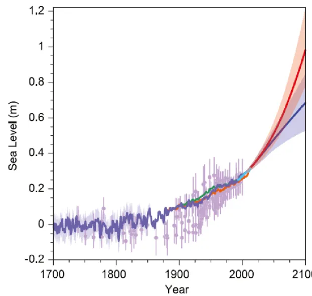
most recent projections by the IPCC (IPCC, 2014) consider a scenario of very high emissions,
47
and predict a global rise of 52–98 cm by the end of this century, which would threaten the
48
viability of many coastal cities (Fig. 1).
49
What matters most to the coastal morphological equilibrium is not the global-mean
50
projected SLR rate itself, but the local change in the observed relative sea-level rise (RSLR).
51
Possible causes of regional sea-level variations include gravitational effects resulting from
52
land ice mass changes, thermal expansion, and ocean dynamics (Slange et al., 2012). RSLR
53
has already been identified in the literature (e.g., Church and White, 2006; Kirwan and
54
Murray, 2008; Kirwan et al., 2008; Chust et al., 2009; Gillanders et al., 2011) as a critical
55
variable for the establishment and maintenance of biotic coastal communities, as a threat to
56
biodiversity, and as being responsible for the increasing magnitude and spatial extent of storm
57
surge flood hazard, amongst other issues. Indeed, the impacts of RSLR are already evident in
58
several different coastal regions (e.g., IPCC, 2007; Nicholls et al., 2007; Fitzgerald et al.,
59
2008). However, regarding morphological feedback, there is still a lack of critical
60
examination of the dimensions of change to come (Orford and Pethick, 2006). Perhaps the
61
most serious and widely recognized issue facing coastal conservation is the impact of RSLR
62
on coastal landforms in coastal lagoons and estuaries. Coastal lagoons are here considered as
63
“inland water bodies separated from the ocean by a barrier, connected to the ocean by one or
64
more restricted inlets which remain open at least intermittently, and have water depths which
65
seldom exceed a few metres” (Adlam, 2014). About 32,000 lagoons are reported along 13% of
66
the world’s coastline (Carter and Woodroffe, 1994), with a coastline contribution estimated at
67
17.6 % for North America, 12.2% for South America, 5.3% for Europe, 17.9 % for Africa,
68
13.8 % for Asia, and 11.4 % for Australia (Barnes, 1980).
69
The size of coastal lagoons varies substantially, with surface areas ranging up to
70
10,200 km2, as in the case of Lagoa dos Patos in Brazil (Pilkey et al., 2009). Coastal lagoons
71
are relatively young features, have formed over the last 5000–7000 years, and are often short
72
lived over geological timescales because of sedimentation (Martin and Dominguez, 1994).
73
Most coastal lagoons are maintained only by the protection afforded by barriers and spits,
74
presenting very peculiar feedbacks to RSLR (List et al., 1997). Although the responses to the
75
effects of RSLR observed in coastal lagoons are manifest in different contexts (e.g., physical,
76
ecological, and economic) and over different time scales, only the physical changes
77
(inundation and sediment supply) are discussed in the present work.
78
Geological observations reveal that many barrier systems worldwide have been able
79
to keep pace with RSLR for thousands of years (McBride et al., 2013). These systems can
80
have spatially distinct responses to RSLR, as in the case of the Gulf of Mexico, which is
81
composed of several bay/lagoon stretches and barriers, where previous studies (e.g., Troiani
82
et al., 2011) have reported rapid and dramatic morphological changes resulting from RSLR
83
but also spatial differences in the response. Other case studies showing the influence of RSLR
84
on lagoons and/or estuaries include Lagoa dos Patos, Brazil (e.g., Toldo et al., 2000), Lake
85
Illawarra and St Georges Basin, New South Wales, Australia (e.g., Sloss et al., 2006), Venice
86
Lagoon, Italy (e.g., Ferla et al., 2007), Pamlico–Albemarle Sound, North Carolina, United
87
States (e.g., Pilkey et al., 2009), Wadden Sea, Netherlands/Germany (e.g., Dissanayake et al.,
88
2012), Ria Formosa, Portugal (e.g., Andrade et al., 2004), Vistula Lagoon, Baltic Sea (e.g.,
89
Navrotskaya and Chubarenko, 2013), and Manzala Lagoon, Egypt (Frihy and El-Sayed,
90
2013).
91
In addition to the direct link between RSLR and physical systems, morphological
92
changes resulting from RSLR can also lead to drastic consequences in the social–economic
93
frame (Nicholls and Tol, 2006). Anthoff et al. (2006), in a study dedicated to all types of
94
coast, detailed the economic and social implications of large rises in sea level during the
95
twenty-first century and beyond (the main outcomes are shown in Fig. 2). Those authors
96
estimate that 145 million people live within 1 m of present-day mean sea level. Regionally,
97
the most threatened lands are North America, central Asia, and unpopulated Arctic coastlines.
98
In terms of threatened population, eastern and southern Asia dominates (Fig. 2) owing to their
99
large populated delta areas. In terms of economies, eastern Asia, Europe, and North America
100
dominate, although this distribution most likely will change during the twenty-first century
101
(Anthoff et al., 2006).
102
Understanding how RSLR is likely to affect coastal regions (in particular lagoons)
103
and consequently how society will choose to address this issue in the short term in ways that
104
are sustainable for the long term, is a major challenge for both scientists and coastal
policy-105
makers and managers (CCSP, 2009). The need for adaptation to climate change is evident,
106
and much more research is still required if our understanding of these important issues is to be
107
refined. According to Nicholls et al. (2006), the average annual costs for protecting coastlines
108
are assumed to be a linear function of the rate of RSLR and of the proportion of the coast that
109
is protected. The costs increase by an order of magnitude if the rate of RSLR is higher than 1
110
cm yr−1 (i.e., protection costs are much higher for the 1 m and 2 m rise scenarios than for the
111
0.5 m scenarios). Therefore, to predict impacts, we need to be aware of changes (Nicholls and
112
Tol, 2006; Woodroffe and Murray-Wallace, 2012). Several questions still need to be
113
answered, the most important of which are: To what extent are the observed changes locally
114
important from the natural and social–economic–cultural points of view? And, to what extent
115
will global mitigation measures prove adequate for local cases? These questions are often
116
associated with a difficulty in conceptualizing and quantifying the main expected responses
117
(from the natural and social–economic–cultural points of view).
118
The present work reviews the previous research on coastal lagoon evolution
119
associated with RSLR and discusses the main modelling attempts for forecasting induced
120
changes in coastal lagoon systems. This review is oriented more towards the most relevant
121
papers on the topic of SLR and induced morphological changes inside coastal lagoon systems.
122
Therefore, emphasis is placed on the physical constraints (morphological changes in intertidal
123
areas) rather than on the biological/ecological processes or social–economic––cultural
124
consequences. Three foci to the review are presented: (a) summarizing the main approaches
125
used in predicting medium- to long-term trends in SLR; (b) identifying the main evolutionary
126
trends of coastal lagoons and the tools used to examine such trends; and (c) highlighting the
127
aspects that require further research.
128
129
2. SLR scenarios and key uncertainties
130
There has been much discussion about projected (and the sources of projection) vs.
131
measured SLR rates. Which rates should coastal scientists and managers apply in their
132
studies, and what is the degree of confidence of such forecasts, are still open questions. Most
133
of the studies conducted on these aspects have been based on scenarios, which allow
134
assessments to be made of developments in complex systems that are either inherently
135
unpredictable or which have high scientific uncertainties. The reliability of and the difficulties
136
associated with the development and use of scenarios have emerged as important problems
137
for and constraints on impact and adaptation studies (Nicholls et al., 2014). As an example,
138
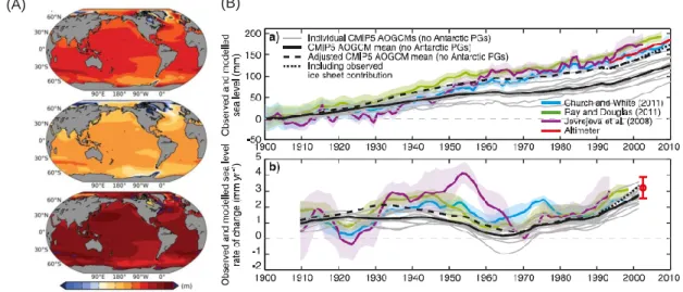
Figure 3A illustrates the SLR scenario variability for the end of this century (period 2081––
139
2100) for just one (RCP4.5, RCP – representative concentration pathway) of the recent SLR
140
projections released by IPCC (2014); the three panels clearly show different sea-level
141
changes, dependent on the model uncertainty.
142
In the overall context of SLR forecasts, two inherent uncertainties are involved. The
143
first (the ‘scenario uncertainty’) arises from our limited knowledge of the future social,
144
economic, and technological development of the world, and of the consequent greenhouse-gas
145
emissions. Therefore, a range of plausible scenarios has been used to describe the way in
146
which emissions may change in the future. The second uncertainty (the ‘model uncertainty’)
147
is related to shortcomings in the present knowledge of the science of climate change, due
148
partly to the fact that we do not know exactly the present climate state (the ‘initial
149
conditions’), and due partly to the fact that no model provides a perfect representation of the
150
real world (Hunter, 2010).
151
Although there are yet no complete simulations of regional ocean temperature
152
changes and of the response of ice sheets to realistic climate change forcing, publications to
153
date have allowed an assessment of the likely range of SLR for the twenty-first century
154
(IPCC, 2014). Hindcast predictions computing the sum of observed contributions to SLR are
155
in good agreement with the observed rise (Fig. 3B).
156
Direct comparisons between the values from the IPCC’s 4th assessment report
157
published in 2007 (AR4) and the newly released 5th Assessment Report (AR5; IPCC, 2013
158
and 2014) are difficult, because underlying scenarios have been significantly revised (Horton
159
et al., 2014). The recent AR5 projected a ‘likely’ (i.e., a 66% likelihood range) global-average
160
sea-level rise of 28–61 cm for a scenario of a drastic reduction in emissions (RCP 2.6) and
161
52–98 cm in the case of an unmitigated increase in emissions (RCP 8.5; Table 1; Fig. 1).
162
163
Table 1. Global SLR by the year 2100 as projected by the IPCC’s AR5. The values are
164
relative to the mean for 1986–2005, so 1 cm should be subtracted to obtain values relative to
165
the year 2000 (source Horton et al., 2014).
166
Scenario designation* Mean (cm) Range (cm)
RCP2.6 44 28–61
RCP4.5 53 36–71
RCP6.0 55 38–73
RCP8.5 74 52–98
*for more details about each scenario, please see IPCC AR5 (http://www.ipcc.ch/report/ar5/)
167
168
The key findings of IPCC AR5 for past and future sea levels can be summarized as:
169
(1) global sea level is rising, (2) this rise has accelerated since pre-industrial times, and (3) the
170
rise will accelerate further during this century (in fact, it will continue to rise during the
171
twenty-first century and beyond, as shown in Fig. 3B). For the first few decades of the
172
twenty-first century, regional sea-level change will be dominated by climate variability
173
superimposed on the climate change signal. For an unmitigated future rise in emissions
174
(RCP8.5), IPCC (2014) expects between 0.5 and 1.0 m of SLR by the end of the twenty-first
175
century (Figs 1 and 3B). Taking into consideration the mean SLR for the RCP8.5 scenario
176
(Table 1), the estimate is 74 cm, which means an expected SLR of more than four times larger
177
than that experienced during the twentieth century (17 cm; IPCC, 2014). These scenarios
178
reflect the large inertia in sea-level response: it is difficult for SLR slow down again once it
179
has been initiated (IPCC, 2013).
180
As scientific understanding improves, a common objective is to narrow the range of
181
uncertainty in the predictions of SLR (even in AR5). There still exists a low (but not
182
negligible) risk of much larger rises (>1 m) in sea level, which are of particular relevance to
183
impact and adaptation assessment (Nicholls et al., 2014), and this issue has not yet been
184
resolved by the IPCC. For coastal planning, SLR needs to be considered in a risk management
185
framework, requiring knowledge of the frequency of sea-level variability in future climates,
186
projected changes in mean sea level, and the uncertainty in sea-level projections (Hunter,
187
2012). For coastal evolution, other issues such as the compaction of sediments (and
188
subsidence) and the changing supply of these sediments to maintain the height of coastal
189
systems must also be considered (see Section 3).
190
A persistent major source of uncertainty, in addition to the uncertainty contained in
191
the projected mean SRL values, is how and when SLR will manifest itself at different scales
192
(Nicholls and Klein, 2005), especially at the local scale (RSLR). Assuming that we are
193
prepared to face RSLR, such information is vital to inform policy-makers and
decision-194
makers when determining whether measures have to be taken to protect coastal communities
195
from sea-level rise.
196
Indeed, the IPCC’s projections have been limited to a global mean value and do not
197
consider the large regional variations induced by various other local processes, leading to
198
non-uniform underestimations of RSLR. The results of Slangen et al. (2012), which
199
considered the sea-level scenarios advanced by AR4, show that estimates of RSLR differ
200
substantially from the global mean SLR. The AR5 report underlines that global average
201
projected scenarios are indeed useful approximations that reflect the contribution of climatic
202
processes, and represent good estimates of sea-level change at many coastal locations. At the
203
same time, the IPCC recognizes that the various regional processes can cause large departures
204
from the global average value; however, a comprehensive discussion of this issue is lacking in
205
the report.
206
207
3. Time scales and length scales of coastal evolution
208
The extreme non-linearity of coastal sedimentary systems in coastal lagoons often
209
hinders our ability to make predictions of coastal change at larger scales, particularly because
210
the temporal ‘upscaling’ of processes from smaller scales to those relevant to coastal
211
management (or vice versa) is a difficult (and sometimes ill-advised) practice, and limits our
212
capacity to predict future coastal change (Ashton et al., 2007). Coastal lagoons enclose
213
morphologies presenting different spatial scales, ranging from bed forms (~cm to m) such as
214
ripples and dunes, to channel–shoal patterns, vegetated salt marshes, and full basins (~1–100
215
km, Carter and Woodroffe, 1994; Perillo, 1995; Hibma et al., 2004), which have complex
216
evolutions that do not follow a specific formula or respond in a linear fashion to forcing
217
factors. Barriers and channels are constrained by boundary conditions, and the cycle of
218
evolution taking place is bound by the principle of Markovian inheritance, whereby the
219
product of previous changes (i.e., antecedent topography and hydrology) provides the initial
220
conditions upon which future evolutionary processes build (Cowell and Thom, 1994). Cowell
221
and Thom (1994) developed a very appropriate account of morphodynamic processes and
222
coastal domain evolution with respect to different time and space scales (Fig. 4). Their
223
conceptual model illustrates the interaction between operating hydrodynamic and sediment
224
dynamic processes and the morphology (topography) of the coastal area. In this scheme, the
225
longer-term evolution of a coastal lagoon is a function of RSLR, tide height and asymmetry,
226
the resulting spatial gradients of the tide residual sediment transport, and the sediment
227
input/output budget. However, other processes (such as wind waves, mud, and vegetation
228
growth) may also play a significant role.
229
The present study envisages a large-scale length context (tens to hundreds of km in
230
length) and long-term (decades up to hundreds of years) approaches (Fig. 4). The long-term,
231
large-scale evolution was chosen because lagoon evolution over such temporal and spatial
232
scales has not been widely studied or synthesised. Moreover, the most significant studies and
233
their outcomes are very recent, covering the past two decades, and there is a need to integrate
234
and validate these studies.
235
236
4. Morphological effects of RSLR in coastal lagoons
237
The wide variety of spatial and temporal scales involved in coastal basins makes their
238
morphodynamic long-term behaviour very complex (Dastgheib et al., 2008). The whole basin
239
system (mega-scale), includes barriers, inlets, basins, and marshes, and embraces different
240
morphological elements (macro-scale) and various morphological features inside each
241
element (meso-scale) responding differently, both temporally and spatially, to physical
242
changes (Ranasinghe et al., 2012). The geological evolution of a lagoon is typically expressed
243
in terms of the rate of basin fill through sedimentation. It is thus helpful to consider the
244
lagoon fill in terms of maturity (Roy et al., 2001; Smith, 2001). Immature lagoons are newly
245
inundated depositional basins in which the entire volume of the water body is available to
246
accommodate sediment (i.e., the volume of empty space behind the barrier that would need to
247
be filled with sediment in order to reach sea level, hereafter referred to as accommodation
248
space). In contrast, mature lagoons are entirely filled with sediment, accommodation space
249
has been exhausted, and river discharge flows directly to the coast. Most processes operating
250
within lagoons affect the degree of maturity through the creation and consumption of
251
accommodation space (Adlam, 2014). The rate of consumption of accommodation space is
252
dependent on the rate of sediment supply (Roy et al., 1980; Boyd et al., 1992).
253
4.1. RSLR and the evolution of barriers and inlets
255
As sea level rises, barrier islands tend to migrate (e.g., Hoyt, 1967; Swift, 1975;
256
Bruun, 1988; Zhang et al., 2004; Masetti et al., 2008; Moore et al., 2010). Besides RSLR,
257
other factors that control rates of island migration include the underlying geology (e.g., Riggs
258
et al., 1995), the stratigraphy (e.g., Storms et al., 2002; Moore et al., 2010), sediment grain
259
size (e.g., Storms et al., 2002; Masetti et al., 2008), substrate slope (Storms et al., 2002;
260
Wolinsky and Murray, 2009; Moore et al., 2010), and substrate erodibility (Moore et al.,
261
2010).
262
Although our overall understanding of how barrier islands respond to climate change
263
continues to improve, little is known about how the connectivity of the two constituent
264
landscape systems (i.e., barriers and inlets) affects the evolution of coupled barrier–marsh
265
systems under changing conditions (Walters et al., 2014). Under rising sea level, barriers will
266
lose areal extent at a rate equal to that at which the barrier island rolls over the marsh
267
platform, unless the marsh progrades into the bay or up the mainland slope as it is flooded by
268
the rising sea level (Moore et al., 2014). Recent findings from Watson et al. (2011) and
269
Walters et al. (2014) suggest that barriers backed by marshes have the added benefit of
270
reduced accommodation space, which allows an island to remain “perched” on the marsh,
271
compared to islands backed by open bays, which must migrate further landwards to maintain
272
elevation relative to sea level. In fact, marsh-backed islands appear to be less vulnerable to
273
rising sea level than do bay-backed islands, because they are able to maintain a more offshore
274
position without a significant contribution of sand from alongshore transport or from the
275
shoreface (Walters et al., 2014).
276
An increase in the rate of RSLR will gradually change the hypsometry of the
277
backbarrier, transforming supratidal areas to open-water and intertidal environments, as
278
observed by Ashton et al. (2007). RSLR will cause changes in inlet geometry or in tidal
279
forcing, affecting the baseline level of transport through the inlet, and thus to the interior
280
(Smith, 2001). Figure 5 illustrates the equilibrium volumes of the elements of an inlet as a
281
function of SLR: with a higher rate of RSLR, the dynamic equilibrium volume of the channel
282
increases and the dynamic equilibrium volume of the ebb-tidal delta decreases. Such trends
283
were obtained by van Goor et al. (2003) for the Dutch Wadden Sea (Fig. 5). Those authors
284
assumed the existence of a dynamic equilibrium to predict critical rates of SLR for inlet/basin
285
systems. In the graph, as the sediment demand for a smaller basin decreases, the inlet adapts
286
more easily to a higher rate of sea-level rise, for the same hydrodynamic and sedimentological
287
conditions. For the basins considered, there was a gradual deepening over time of the tidal
288
basin that prompted an importation of sediment (van Goor et al., 2003).
289
Even if detailed descriptions exist of the responses of barrier chains and inlets to
290
RSLR, as well as various attempts to systematize the foreseen impacts, there remains a
291
deficiency in the conceptualization of expected morphological changes and their importance
292
at the regional/local scale that is presented in a straight-forward manner and which can be
293
rapidly assessed by decision-makers. Penland et al. (1988) were amongst the first to
294
conceptualize the long-term scenario response of a low-lying system to RSLR, referring to the
295
system as a delta-type coast (namely, the Mississippi Delta). Focussing more on coastal
296
lagoons, Fitzgerald et al. (2006) developed a conceptual scheme (Fig. 6) that describes the
297
barrier/inlet/basin cell feedback in relation to RSLR, and which can be used to interpret
long-298
term changes in coastal barrier systems. Fitzgerald’s (2006) scheme is more complete and
299
more exhaustive than that of Penland et al. (1988), and has wider application. It addresses the
300
fate of mixed-energy barrier coasts found throughout the northeastern coast of the United
301
States, the East Friesian Islands in the North Sea, and the Copper River delta barriers in the
302
Gulf of Alaska, which are characterized by short, fragmented, stubby barrier islands,
303
numerous tidal inlets, well-developed ebb-tidal deltas, and a backbarrier consisting of salt
304
marshes and tidal flats incised by tidal creeks.
305
In essence, the model of Fitzgerald (2006) represents the conversion of marsh to open
306
water, causing an increase in the tidal prism and growth of the ebb shoals (a stable barrier to
307
transgression, Fig. 6). In the model, no additional sediment inflow is considered, and the
308
greater part of the inorganic sediment input is marine. The loss of marshlands increases tidal
309
exchange between the ocean and backbarrier and ultimately changes the hydraulic regime of
310
the tidal inlets. The growth of both ebb- and flood-tidal deltas diminishes the supply of sand
311
along the coast, leading to a fragmentation of the barrier chain and the formation of a
312
transgressive coastal system (stage 3, Fig. 6). Sand is assumed to be lost from the littoral
313
system as it is moved into the backbarrier to form flood shoals (FitzGerald et al., 2006). There
314
is an increase in the tidal prism, which strengthens the tidal currents and enlarges the size of
315
the tidal inlets. During the process of increasing tidal exchange between the backbarrier and
316
ocean, there is the potential for dramatic changes to occur in the inlet shoreline (stage 2, Fig.
317
6). A change from ebb- to flood-dominated inlets, as the marshes and tidal creeks are
318
transformed to open bays, promotes the formation of flood deltas, but does not retard the
319
growth of ebb deltas, because the volume of the flood deltas is dependent on the tidal prism
320
(FitzGerald et al., 2006).
321
Prior to the study of FitzGerald et al. (2006), FitzGerald et al. (1984) had already
322
illustrated with respect to the evolution of the Friesian Islands what can happen to a barrier
323
chain when an alteration of backbarrier hypsometry induces changes in the tidal prism,
324
although the earlier study did not incorporate a relevant conceptual schematisation. During a
325
310 year period, the backbarrier area of the Friesian Islands decreased by 30% due mostly to
326
land reclamation of tidal flat areas along the landward sides of the barriers and along the
327
mainland shore. Secondary losses were attributed to re-curved spit extension into the
328
backbarrier. These processes resulted in a reduction in the tidal prism and a coincident
329
narrowing of the tidal inlets by 52% (FitzGerald et al., 1984).
330
Most of the findings of FitzGerald et al. (2006) were subsequently corroborated in the
331
case study of Dissanayake et al. (2012). The investigations of Ganju and Schoellhamer (2010)
332
and Dissanayake et al. (2012) were the first to address the morphodynamic impact of RSLR
333
on inlet systems using a numerical model.
334
335
4.2. RSLR, sediment supply, and basin evolution
336
Depending on local basin geometry, RSLR causes sediment import or export (see
337
Friedrichs et al., 1990). In the case of a flood-dominated tidal lagoon, RSLR tends to result in
338
sediment accumulation as a means of restoring the intrinsic dynamic equilibrium of the basin
339
(Dronkers, 1998). Thus, besides the direct barrier and inlet adjustments, RSLR also affects the
340
basin drainage area. Redfield et al. (1965) were the first to provide evidence of concomitant
341
bay infilling and lateral progradation of the intertidal marsh onto sand flats, where existing
342
meandering channels were stabilized by the marsh itself through narrowing of the channels
343
until the flow was concentrated enough to prevent further erosion or deposition.
344
A relevant conceptualization of tidal basin response to accelerated RSLR, using the
345
Wadden Sea as an example, is expressed in Figure 7. The graph in that figure is consistent
346
with the conceptual model proposed by FitzGerald et al. (2006), and highlights the concept of
347
‘adjustment’ inside the tidal basin. The scheme proposed by FitzGerald et al. (2006) is
348
focused mostly on the SLR–inlet–backbarrier relationship, whereas the Louters and Gerritsen
349
(1994) scheme details the steps of adjustment inside the lagoon, namely, regarding the depth
350
of the basin, after an increase in the rate of RSLR. The Louters and Gerritsen (1994) model
351
also assumes that there is a dynamic balance between sediment supply, ecosystems, and
352
changes in sea level; indeed, as stated by the Bruun rule, an equilibrium state is assumed in
353
the periods between sediment basin adjustments to RSLR. Therefore, the system’s response to
354
the rise is delayed and the average basin level thereby becomes slightly lower in relation to
355
sea level. If the sea level rises at an increased rate, the tidal basin deepens slightly over time
356
in relation to the rising sea level. At the beginning of this process, the sand retention capacity
357
of the deepened basin gradually increases (Fig. 7). The total quantity of sand required to
358
restore dynamic equilibrium is directly proportional to the rate of RSLR. If the supply of
359
sediment is not sufficient to allow the tidal area to keep pace with RSLR, dynamic
360
equilibrium cannot be regained. In that case, the level of the lagoon will gradually lag behind
361
the rise in sea level, eventually bringing about the area’s inundation (Louters and Gerritsen,
362
1994). The findings of Louters and Gerritsen (1994) were subsequently discussed in the study
363
of Gerritsen and Berentsen (1998), who modelled sediment balance in the wider North Sea
364
Basin for the Holocene SLR, but for a single tidal basin scale.
365
Other recent and relevant studies of basin evolution include the work of Defina et al.
366
(2007), who developed a conceptual model for Venice Lagoon, showing the same patterns of
367
evolution described in Louters and Gerritsen (1994). Such studies also include the work of
368
Lopes et al. (2011), who applied the morphodynamic model MORSYS2D to Ria de Aveiro,
369
and described impacts of RSLR on lagoon hydrodynamics that included an increase in the
370
tidal prism at the lagoon mouth of about 28%, as well as an intensification in sediment fluxes,
371
and, consequently, bathymetric changes. More recently, Dissanayake et al. (2012) modelled a
372
typical large inlet/basin system, the Ameland Inlet, over a 110 year study period, and found
373
an existing flood dominance of the system with increasing rates of RSLR, caused by erosion
374
of the ebb-tidal delta and accretion of the basin. Van der Wegen et al. (2013) showed that the
375
intertidal area might disappear under realistic RSLR rates, with the basin shifting from a
376
sediment-exporting system to an importing system, as well as the basin ‘drowning’ and a
377
considerable reduction in the extent of intertidal areas.
378
The recent review by Coco et al. (2013) of the morphodynamics of tidal networks
379
discusses tidal drainage accommodation space and how tidal channels increase in both width
380
and depth as a result of RSLR and related changes in the flowing tidal prism. Stefanon et al.
381
(2012) provided similar findings, reporting a linear relationship between the tidal prism and
382
the drainage area of the basin, and showing that a decrease in the tidal prism leads to smaller
383
channel cross-sections and a general retreat of the channels, whereas the opposite effect
384
(network expansion and larger cross-sectional channel areas) occurs when the tidal prism
385
increases.
386
387
4.3. RSLR and salt marsh evolution
388
The presence of a marsh platform reduces basin accommodation space as a barrier
389
migrates across the backbarrier region in response to RSLR. Therefore, a good way of
390
predicting the maturity of coastal lagoons is to evaluate salt marsh accumulation rates.
391
Furthermore, salt marsh accumulation rates are also reliable proxies for estimating past RSLR
392
rates (e.g., Edwards, 2007; Cronin, 2012).
393
Marshes cover extensive areas of estuarine and deltaic environments in mid- to high
394
latitudes and support different vegetation types, and also show different rates of inundation
395
and suspended sediment delivery (e.g., FitzGerald et al., 2006; French, 2006; Cronin, 2012).
396
In addition to their dependence on RSLR, the success of marsh maintenance also depends
397
upon other factors such as sediment supply and tidal range (Reed, 1995). Rising water levels
398
could potentially alter the inundation regime in salt marsh habitats, leading to irreversible
399
states. Rizzetto and Tosi (2012) found that both RSLR and the frequency of high tides at
400
Venice Lagoon greatly influenced shifts in the margins of the salt marsh and the meander
401
evolution of tidal channels in the long term, but short-term changes in creek sinuosity were
402
often also closely related to variations in tidal range. The retreat of marsh margins, the
403
increase in network density, and the decrease in creek sinuosity provided evidence for tidal
404
channel development in a regime of RSLR and an increasing strength and frequency of high
405
tides (Rizzetto and Tosi, 2012).
406
The physical responses of salt marshes to RSLR have been frequently coupled with
407
morphological models (e.g., Schwimmer and Pizzuto, 2000; Mariotti and Fagherazzi, 2010;
408
Coco et al., 2013). Recent studies have aimed to improve understanding of the morphological
409
development of marshes by considering factors such as the rate of RSLR, the depth of
410
inundation, inorganic sediment supply, plant productivity, and the accumulation of organic
411
material (e.g., Fagherazzi and Sun, 2004; D’Alpaos et al., 2005; Kirwan et al., 2008). In these
412
models, morphological changes are based on the balance between erosion (dependent on
413
shear stress criteria), inorganic accretion, and organic production, as found from empirical
414
relationships (Morris et al., 2002). Furthermore, successive versions of the sea level affecting
415
marshes model (SLAMM) have been used to estimate the impacts of SLR along the coasts of
416
the United States (e.g., Titus et al., 1991; Craft et al., 2009; Traill et al., 2011; Glick et al.,
417
2013). Besides numerical modelling, other approaches have been used to determine the
418
response of salt marshes to RSLR. For example, using a lab flume experiment, Stefanon et al.
419
(2012) explored the morphological impact of sea-level fluctuations (both decrease and rise)
420
on a tidal network pattern, and demonstrated rapid network adaptation as a result of varying
421
mean water levels and associated tidal prisms. Simulations of these interactions show that salt
422
marshes are able to keep up with RSLR (e.g., Kirwan et al., 2010).
423
In fact, the published model results show that salt marshes are constantly adjusting
424
towards a new equilibrium (Morris et al., 2002); therefore, the interplay between sediment
425
dynamics and the rate of RSLR has been suggested as being critical for the establishment of
426
the equilibrium intertidal area configuration (Marani et al., 2007). This has lately also led to
427
the idea that salt marshes barely attain equilibrium but rather continuously lag and attempt to
428
readjust to changes in sea level (Kirwan and Murray, 2008). Their ability to rapidly accrete
429
vertically and horizontally under favourable conditions reinforces the notion that natural
430
marshes can quickly respond to external forcing (Friedrichs and Perry, 2001; van Wijnen and
431
Bakker, 2001). Marshes will be under severe stress only if the supply of sediment and the
432
build-up of organic material cannot keep up with rising sea level (e.g., Morris et al., 2002;
433
Nielsen and Nielsen, 2002; Temmerman et al., 2004; French, 2006; Kirwan and Temmerman,
434
2009; Andersen et al., 2011). For instance, the recent expansion of water-logged panes in salt
435
marshes in the northeastern United States has been attributed to tidal flooding associated with
436
accelerated rates of RSLR (Hartig et al., 2002). Sediment supply reduction and increased
437
subsidence rates were partially responsible for the reductions in the extent of marshland in
438
Chesapeake Bay and Venice lagoon marshes (Reed, 1995; Day et al., 1998; Marani et al.,
439
2007).
440
Salt marsh growth and development substantially alters the sedimentary processes
441
occurring in lagoons (Fagherazzi et al., 2012; Coco et al., 2013). Herein, we propose a generic
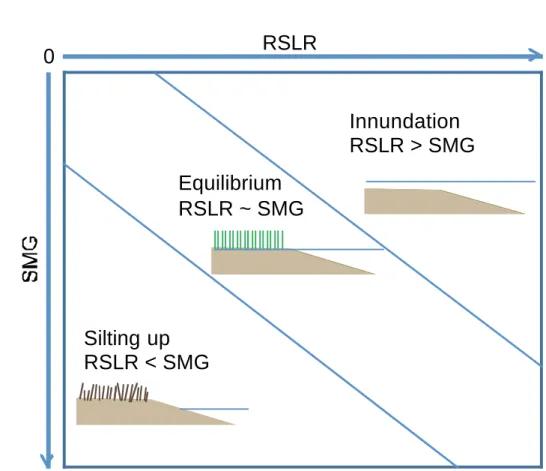
442
conceptual scheme illustrating salt marsh development with respect to RSLR (Fig. 8). It is
443
assumed that the salt marsh accretion rate is the net product of sediment deposition and
444
physical compaction (Bartholdy et al., 2004). Essentially, RSLR is portrayed as creating
445
accommodation space in which fine-grained sediments can settle (sediment supply rate), so
446
that increases in the rate of RSLR theoretically lead to concomitant changes in the rates of
447
mineral sediment deposition (in agreement with the results of Redfield, 1972); however,
448
under high rates of RSLR, with an insufficient supply of sediment and organic material,
449
inundation of the salt marsh will occur. In contrast, if the rate of sediment supply is much
450
higher than the rate of RSLR, silting-up dominates and the marsh will shift towards a
451
different environment and ecosystem (an infilling lagoon).
452
Assuming a sufficient supply of sediment, and after an initial phase of growth, the
453
SMG (salt marsh growth) rate will tend to attain equilibrium with the rate of RSLR (Fig. 8,
454
central panel), and the salt marsh surface, also referred to as the marsh platform, will be at a
455
level between near mean high tide (Krone, 1987) and just below the highest (astronomical)
456
tide (Allen, 2000). The elevation of the platform relative to sea level determines the total
457
wetland area, inundation frequency and duration, and wetland productivity (Morris et al.,
458
2002).
459
If SMG rates are too low to keep pace with the rate of RSLR (slow growth as result
460
of low silt input), the intertidal area in the lagoon is dominated by inundation, and there is no
461
effective salt marsh development (Fig. 8, upper panel). If the amount of inundation becomes
462
sufficient to stress or kill vegetation, then the marsh substrate begins to break up as peat
463
collapses: salt marshes cannot adapt and may drown, the lower part of the substrate may
464
become eroded (Kirwan et al., 2010; Cronin, 2012), and inner channel networks will expand
465
(Hartig et al., 2002). There is no predefined time lag applying to when the marsh substrate
466
begins to break up (or recover), and future research must seek to estimate the capacity for
467
resilience of these areas. This threshold appears to have already been reached for many of
468
coastal Louisiana’s wetlands, owing to a number of anthropogenic and natural factors
469
(Morton et al., 2005). In contrast, if SMG rates are higher than rates of RSLR (rapid growth
470
as result of excessive silt input), the intertidal area becomes sediment saturated and the salt
471
marsh will shift horizontally if there is enough accommodation space (Fig. 8, lower panel).
472
The process leads to a loss of inner-basin area and a continuation of infilling, resulting in salt
473
marsh decay over the long term.
474
The two extreme conditions portrayed above bear negative impacts on the extent of
475
both salt marshes and basins. Determining the clear effects of each of them remains difficult,
476
because the effects of RSLR alone cannot be isolated in natural wetlands. Even if we presume
477
that vertical accretion in salt marshes is solely a function of inorganic and organic matter
478
influx and ignore the effects of regional subsidence along coastlines, it is clear that many
479
marshes will not be able to keep up with the projected increase in the rate of SLR forever,
480
which might result in the partial conversion of marshlands to subtidal and unvegetated
481
intertidal areas (Ashton et al., 2007). The ultimate submergence of coastal marshes occurs
482
when there is insufficient elevation to prevent excessive waterlogging of the marsh soil (as
483
observed by Reed (2002) in the Mississippi salt marshes).
484
Day et al. (1998) compiled information about salt marsh accretion rates, reporting a
485
vertical accretion rate of 0.3–2.3 cm yr−1 in Venice lagoon as measured over two years.
486
FitzGerald et al. (2006) reported an interval of 0–14 mm yr−1, with a mean rate of 5.0 mm
487
yr−1. Pethick (1992) measured accretion rates of >2.0 cm over two years in a salt marsh in
488
England, although this was not specifically for a coastal lagoon. Assuming the IPCC’s mean
489
estimate of 74 cm (9 mm yr−1) of SLR by the end of this century for the RCP8.5 scenario, and
490
a salt marsh average accretion rate of 5.0 mm yr−1 (assuming the mean rate of FitzGerald et
491
al., 2006), the amount of SMG will be (on average) lower than the amount of RSLR, and
492
intertidal lagoons will be prone to inundation. In a large number of coastal systems
493
worldwide, the accretion will be insufficient to prevent water-logging of marsh soil, leading
494
to plant deterioration. This could be particularly relevant by the end of the twenty-first
495
century, because the overall 74 cm of SLR includes an acceleration in SLR from the present
496
day until the end of the century. The exceptions would be places with high availability of
497
sediment, where salt marshes can survive under a rate of RSLR in excess of 1 cm yr−1 (as
498
observed in the Mississippi delta by Reed, 2002).
499
The adjustment of salt marshes to RSLR also depends on the acceleration of sea-level
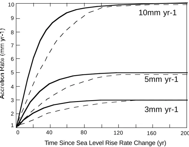
500
rise. The experimental results of Kirwan and Temmerman (2009), as illustrated in Figure 9,
501
help to quantify the strength of the lagoon inundation–accretion feedback and the response of
502
marsh accretion rates to step-by-step changes in the rate of RSLR. The results of Kirwan and
503
Temmerman (2009) suggest that regardless of the magnitude of change, a marsh adjusts to a
504
change in the rate of RSLR within about 100 years (returns to equilibrium, Fig. 9). Sediment
505
availability is assumed, and the forecast accretion occurs because a feedback is considered
506
between inundation and suspended sediment concentrations (sediment deposition rates are
507
proportional to inundation depth) that allows marshes to quickly adjust their elevation to a
508
change in the rate of sea-level rise. The long-term behaviour as suggested by the experiments
509
of Kirwan and Temmerman (2009) fits some of the behaviours observed in the Louisiana
510
wetlands (DeLaune et al., 1994), but does not match other response scenarios such as the
511
expansion of drainage networks of tidal creeks in Cape Romain, South Carolina (Hughes et
512
al., 2009).
513
Abiotic parameters also control salt marsh responses. Riverine-dominated salt
514
marshes (such as many Gulf Coast and Chesapeake Bay marshes) experience greater
515
sediment accumulation as a result of enhanced input of inorganic sediment compared with
516
marshes, where the major source of inorganic sediment is marine (FitzGerald et al., 2006).
517
Lagoon marshes that do not experience significant fluvial delivery of inorganic sediment may
518
therefore be at greater risk of inundation with rising sea level, as the main source of inorganic
519
sediment to these marshes is the ocean, via tidal inlets. In coastal lagoons and estuaries, an
520
absolute increase in the elevation of the marsh platform in response to rising sea level should
521
cause a landward migration of the marsh (Gardner and Porter 2001), and this may change the
522
areal extent of wetland and consequently total production, depending on local geomorphology
523
and anthropogenic barriers to migration.
524
525
5. Modelling the evolution of coastal lagoons under RSLR scenarios
526
Numerical models have proved to be fundamental tools for gaining insights into
527
barrier evolution and resilience, and have evolved significantly in the last 20 years. They have
528
been developed and validated mostly for ocean front beaches and have only rarely been
529
applied to the overall evolution of coastal lagoons. Indeed, there is a lack of model predictors
530
adapted to the study of coastal embayments and lagoons. The following review is therefore
531
focused on morphodynamic models that are commonly used in coastal applications, but which
532
have apparent applicability to coastal lagoons.
533
Models relating SLR and coastal evolution have been developed for making
long-534
term predictions, and in the last 20 years have experienced huge improvements in complexity,
535
applicability, and reliability. Such models can be split into three main groups: simple
536
shoreline models, behaviour models, and process-based models. These models can be applied
537
at various degrees of dimension. One-dimensional models are ideal for studying, for example,
538
width-average equilibrium profiles; two-dimensional models account for the formation of
539
depth-averaged features (e.g., a channel or shoal); and three-dimensional models additionally
540
account for small-scale hydrodynamic changes in the vertical dimension, that is, due to
541
curvature or density gradients (Hibma, 2004; Lesser et al., 2004).
542
The older and most widely used sandy shoreline response models include the Bruun
543
rule (Bruun, 1962) and modifications to the Bruun rule (e.g., Dubois, 1992; Davidson-Arnott,
544
2005). Several studies claim to have demonstrated the applicability of the Bruun rule (e.g.,
545
Leatherman et al., 2000; Zhang et al., 2004), and, perhaps because of its elegant simplicity, its
546
use has become commonplace by coastal planners and managers (Pilkey and Cooper, 2004).
547
In the last 10 years, criticisms of the Bruun rule have been many and varied (e.g., Sallenger,
548
2000; Cooper and Pilkey, 2004). Several authors have pointed out that this principle is
549
applicable only to a restricted number of beaches (coasts without net alongshore sediment
550
transport; Brunel, 2009). Consequently, several modifications to the Bruun rule have been
551
made in attempts to attain greater accuracy in representing the response of the beach profile to
552
SLR (e.g., Komar et al., 1991; FitzGerald et al., 2008; Rosati et al., 2013).
553
During the 1990s, a suite of quantitative morphological behaviour models was
554
developed, namely, the large-scale coastal behaviour (LSCB) models. Behaviour models are
555
used to simulate the large-scale morphological and stratigraphic evolution of coasts that
556
occurs as a result of changes in sea level and in sediment supply (e.g., Cowell et al., 1995;
557
Niedoroda et al., 1995; Stive and de Vriend, 1995). Similar to the way in which shoreline
558
response models use time as a surrogate for processes, the LSCB models utilize geometric
559
cross-shore profile parameters as proxies for processes. As an example, the Integrated
560
Assessment Models (IAMs) appeared at the beginning of the twenty-first century and are used
561
to evaluate the vulnerability of coastal systems to multiple climate change impacts. The
562
ability to achieve a fully integrated assessment of coastal vulnerability, considering dynamic
563
interactions between sectors and/or processes, makes IAMs very useful in supporting policy-
564
and decision-making at various scales. However, given the complex nature of such models,
565
their implementation requires significant expertise. FUND, DIVA (Dynamic interactive
566
assessment model), SimCLIM, and RegIS (Regional Impact Simulator) are examples of IAMs
567
dealing with the valuation and management (in terms of adaptation) of multiple climate
568
change impacts on coastal areas and related ecosystems (see Hinkel, 2005; Holman et al.,
569
2008; Warrick, 2009; Mcleod et al., 2010). For example, FUND is an integrated assessment
570
model with a coastal impact component that includes country-level cost functions for dry land
571
loss, wetland loss, forced migration, and dike construction (Tol, 2007); it works at the sector
572
level, so that economic costs can be estimated for SLR. DIVA is a dedicated coastal impact
573
model employing subnational coastal data (Vafeidis et al., 2008), and considers additional
574
impacts such as coastal flooding and erosion as well as adaptation in terms of protection via
575
dikes and nourishment (Hinkel and Klein, 2009). DIVA assesses coastal flood risk based on
576
the hydrological elevation and extreme water level distributions (Hinkel et al., 2013) and
577
erosion based on a combination of the Bruun rule and a simplified version of the ASMITA
578
(Aggregated Scale Morphological Interaction between Tidal inlet and Adjacent coast) model
579
for tidal basins (Nicholls et al., 2011).
580
In clear contrast to the aforementioned behaviour models are the 2D process-based
581
models and the recent 3D circulation process-based models, which when coupled with
582
sediment transport processes demonstrate success at modelling hydrodynamics and
583
morphology over shorter time scales (Lesser et al., 2004; Roelvink 2006). Process-based
584
models consider changes in the patterns of circulation inside coastal basins (McLeod et al.,
585
2010), portraying different coastline changes and tidal sedimentation scenarios along the
586
same coastal system. Although not specifically developed to deal with climate change
587
impacts, these models can be applied to sector analysis (e.g., shoreline change and storm
588
impact simulations) or to the integrated assessment of coastal vulnerability to SLR. The main
589
examples include Delft3D, developed by Deltares (e.g., Lesser et al., 2004; Tung et al., 2009;
590
van der Wegen and Roelvink, 2012), MIKE 2D, and the KUTM (the Kyushu University Tidal
591
Model). Comprehensive morphodynamic modelling systems such as ECOMSed, Mike-21,
592
Delft3D ROMS, and TELEMAC–MASCATE (Hervouet and Bates, 2000;
593
http://www.opentelemac.org) generally include different flow modules (from 1D to 3D), a
594
wave propagation model, and a sand transport model including bed load and suspended load
595
(Villaret et al., 2013; see the example in Fig. 10), which allow integrated modelling of
596
complex coastal systems to be performed at different time scales. Van Dongeren and de
597
Vriend (1994), Stive and Wang (2003), and van Goor et al. (2003) have shown that this type
598
of model has the capacity to predict the decadal-scale morphodynamic development of coasts,
599
including the impact of SLR.
600
With the development of process-based models, the coastal research community
601
experienced a proliferation of numerical method applications. Although this approach
602
requires a higher level of input data compared with the behaviour models, the output of
603
process-based models provides more detailed information on governing processes (van der
604
Wegen et al., 2013). Filtering methods such as tide lengthening or the use of the so-called
605
morphodynamic factor have been extensively applied to reduce computational costs for
long-606
term applications, but such methods also introduce an additional source of uncertainty (van
607
der Wegen and Roelvink, 2008). Many of the models traditionally used to study coastal
608
processes made, by necessity, critical simplifying assumptions that limit their applicability
609
(Ashton et al., 2007). Oversimplification, limited observations, and unknowable future
610
conditions still limit models’ ability to make quantitative reliable predictions.
611
The existing limitations of process-based models concerning the predictability of
612
morphological variables because of the non-linearity of many coastal systems has recently
613
encouraged the development of ‘hybrid models’ (featuring elements of both top-down and
614
bottom-up models) with simplified dynamics that are designed to predict qualitative
615
behaviour by including only predominant processes (Karunarathna et al., 2008). Recent
616
experimentation includes the model types proposed by Karunarathna et al. (2008) and
617
Townend (2010) for estuaries and tidal inlets. Bayesian networks have also been applied to or
618
can provide probabilistic predictions of shoreline change rates using readily available data on
619
driving forces (rate of sea level rise, wave height, tidal range) and boundary conditions (e.g.,
620
geomorphological setting, coastal slope) (see Gutierrez et al., 2011).
621
A problem highlighted in all research pertaining to morphodynamic modelling is that
622
of the accuracy and verification of results or predictions arising from the numerical
623
calculations. The nature of modelling for predicting future change means that until the
624
predicted change takes place, the model cannot be deemed to be ultimately accurate. The use
625
of models to explore and simulate the operation of contemporary processes in natural science
626
can be an important tool if used wisely and while accounting for limitations and the quality of
627
data required for parameterisation (e.g., Roelvink and Reniers, 2012). However, their use as a
628
long-term, large-scale predictive tool is in its infancy and therefore their value is expected to
629
substantially improve in the future.
630
631
6. The economic and social consequences of RSLR for coastal lagoons
632
A given rate of SLR can have differential impacts on economic and social systems
633
depending on where the rise occurs and which population groups are affected. Where
634
exposure and vulnerability are high, even non-extreme events can lead to serious
635
consequences (IPCC, 2013; Felsenstein and Lichter, 2014). Thus, the relative burden of
636
coping with the effects of RSLR is more important from a socioeconomic perspective than is
637
the absolute size of the event (Felsenstein and Lichter, 2014). There are no specific studies on
638
human vulnerability to the expected SLR in coastal lagoons (even in AR4 or AR5), only a
639
few case study examples. For instance, in the absence of anthropogenic barriers, a 1 m rise in
640
sea level would create around 11,000 km2 of new intertidal area in the conterminous United
641
States alone (Morris et al., 2012; Kirwan and Megonigal, 2013).
642
The availability of regional-scale comprehensive vulnerability assessment studies,
643
which are required by local stakeholders for designing adaptation strategies at the local level,
644
is limited (Cooper et al., 2008). Only recently have studies reported human impacts and
645
coastal lagoon management implications arising from RSLR. Cooper et al. (2008) evaluated
646
coastline displacement and its consequences based on the direct inundation of Delaware Bay
647
(New Jersey), and listed the methodologies that may prove useful to policy-makers despite
648
the large uncertainties inherent in the analysis of the local impacts of sea-level change.
649
Carrasco et al. (2012) assessed the inundation of backbarriers and proposed several human
650
adaptation measures, focusing mostly on sandy stretches. Raji et al. (2013) used GIS
651
techniques to assess the number of people at risk from flooding, and constructed a
socio-652
economic vulnerability index according to the distribution of the land uses across physical
653
vulnerability classes. The relatively small number of studies integrating human impacts and
654
morphodynamic evolution induced by RSLR is perhaps because of our need to continue
655
learning how to interpret SLR itself as well as the associated coastal evolution (Ward et al.,
656
2012). Although the study of Cooper and Lemckert (2012) was not exclusively dedicated to
657
coastal lagoons, it highlighted some of the practical considerations that specifically
658
characterize large coastal resort cities. Yoo et al. (2011) developed a methodology for
659
assessing vulnerability to both climate change and RSLR in coastal cities. Other pertinent
660
examples of economic estimates of material losses caused by the consequences of
661
morphodynamic readjustments to RSLR can be found in Ribbons (1996), Anthoff et al.
662
(2010), Merz et al. (2010), and Le Van Thang et al. (2011), who examined the direct link
663
between poverty and RSLR in the lagoons and coastal areas of Thua Thien province,
664
Vietnam.
665
The small size and dispersed distribution of coastal lagoons along coastlines can lead
666
to their mismanagement. In addition, administrative frontiers often do not facilitate a coherent
667
management of coastal lagoons (Gaertner-Mazouni and De Wit, 2012). The main economic
668
and social approaches used to face RSLR rely fundamentally on the adaptation and mitigation
669
options. Clearly important for the definition of adaptation measures is to better understand the
670
links between barrier systems, lagoon marshes, and tidal basins (Ashton et al., 2007), and
671
human frame, and how these features will evolve during RSLR. According to the United
672
Nations International Strategy for Disaster Reduction (UNISDR, 2009), adaptation is ‘the
673
adjustment in natural or human systems in response to actual or expected climatic stimuli or
674
their effects that moderates harm or exploits beneficial opportunities’. Some researchers view
675
society as the adaptive unit; that is, adaptation is the ability of a system to return to
676
functionality. Others perceive the unit of adaptation as being the largest and most inclusive
677
group that makes and implements decisions with respect to exploitation in the habitat
(Oliver-678
Smith, 2009). In contrast to adaptation, mitigation is the ‘lessening or limitation of the
679
adverse impacts of hazards and related disasters, and encompasses engineering techniques
680
and hazard-resistant construction as well as improved Env.al policies and public awareness’
681
(UNISDR, 2009). Mitigation is proactive and increases the resilience of a society; that is,
682
increasing the capacity to absorb the impacts of hazards that exist in its surroundings without
683
major disruption of basic functions. Even with RSLR mitigation measures, coastal adaptation
684
remains essential (Nicholls et al., 2007). The growing populations and economies of the
685
coastal zone reinforce this need. However, the simple implementation of an adaptation
686
measure is not an endpoint; rather, adaptation is an ongoing process requiring the constant
687
prioritisation of risks and opportunities, the implementation of risk-reduction measures, and
688
reviews of their effectiveness. Hence, the performance of any adaptation measure (within the
689
scope of an integrated coastal zone management framework) should be carefully monitored
690
during its implementation to improve its maintenance and other future interventions (UNEP,
691
2010). Only ‘no-regret’ strategy measures (providing economic and environmental benefits
692
by fostering innovation and economic development) and ‘insurance’ responses by the
693
insurance industry (dealing with the precautionary principle where RSLR would have large
694
costs) will be appropriate in the next few decades as coastal management actions (Nicholls