MARINE ECOLOGY PROGRESS SERIES Mar Ecol Prog Ser
Vol. 513: 155–169, 2014
doi: 10.3354/meps10987 Published October 22
INTRODUCTION
Marine protected areas (MPAs) have become a key spatial management and conservation tool for coastal nations worldwide, but their effectiveness is largely uncertain in most, if not all, cases (Kaiser 2011). In fact, the size of the areas where the different species are effectively protected and the amount of time they are available to the fishery is typically unknown.
The adequate design and management of MPAs is highly dependent on the quality of the baseline eco-logical information. Of particular relevance is the knowledge of the species’ site fidelity, distribution and habitat use (Glazer & Delgado 2006, Le Quesne & Codling 2009, Grüss et al. 2011, Schmiing et al. 2013). These data can not only help determine the initial location and correct size of MPAs based on the
species’ habitat requirements but also provide rele-vant information for the adaptive management of already implemented MPAs.
Recent studies have presented quantitative models to assess the efficiency of MPAs (Walters et al. 2007, Le Quesne & Codling 2009, Moffitt et al. 2009). How-ever, these models do not consider that no-take areas do not, in most cases, consist of 100% of suitable habitats. It is therefore possible that a no-take area several times larger than the species’ home range does not offer adequate protection.
Acoustic telemetry is one of the most widely used methods to track marine species, as it provides long-term, fine-scale spatio-temporal data on individual movement and home range (e.g. Afonso et al. 2009, Abecasis et al. 2013b). However, there is no consen-sus on how to translate such individual data, the
typ-© Inter-Research 2014 · www.int-res.com *Corresponding author: [email protected]
Combining multispecies home range
and distribution models aids assessment
of MPA effectiveness
David Abecasis
1,*, Pedro Afonso
2, 3, Karim Erzini
11Centre of Marine Sciences (CCMAR), University of the Algarve, Campus de Gambelas, 8005-139 Faro, Portugal 2Institute of Marine Research, Department of Oceanography and Fisheries, University of the Azores, 9901-862 Horta, Portugal 3Laboratory of Robotics and Systems in Engineering and Science (LARSyS), Avenida Rovisco Pais, 1, 1049-001 Lisboa, Portugal
ABSTRACT: Marine protected areas (MPAs) are today’s most important tools for the spatial management and conservation of marine species. Yet, the true protection that they provide to indivi -dual fish is unknown, leading to uncertainty associated with MPA effectiveness. In this study, con-ducted in a recently established coastal MPA in Portugal, we combined the results of individual home range estimation and population distribution models for 3 species of commercial importance and contrasting life histories to infer (1) the size of suitable areas where they would be fully pro-tected and (2) the vulnerability to fishing mortality of each species. Results show that the relation-ship between MPA size and effective protection is strongly modulated by both the species’ home range and the distribution of suitable habitat inside and outside the MPA. This approach provides a better insight into the true potential of MPAs in effectively protecting marine species, since it can reveal the size and location of the areas where protection is most effective and a clear, quantitative estimation of the vulnerability to fishing throughout an entire MPA.
KEY WORDS: Cuttlefish · Maxent · Marine reserve · Sole · Vulnerability to fishing · White seabream
ical output of telemetry studies, into the more rele-vant population-scale projection when evaluating the effectiveness of protection provided from existing MPAs or forecasting their optimal designs.
This study offers evidence that home range areas and habitat suitability should be addressed when designing MPAs. This was achieved by combining information about species home range areas with species distribution models to calculate the effective protection provided to 3 species with contrasting life histories by a small coastal MPA, the Luiz Saldanha Marine Park (LSMP), Portugal. In particular, this study focused on analysing the vulnerability to fish-ing of the 3 species — cuttlefish Sepia officinalis, Sene-galese sole Solea senegalensis and white seabream Diplodus sargus — and on estimating the size of suit-able areas where these species are in fact protected from local fisheries. Arguably, an MPA design based on the requirements of only 3 species is unlikely to ensure the full protection of all local marine species. Nevertheless, the contrasting life histories of these 3 species, all of which are also of key commercial im -portance for the region, ensure the wide spectrum needed to demonstrate the wider applicability of this study towards this MPA. This study is also innovative in combining typical finfish with cephalopods and flatfishes, which are seldom used in MPA studies (Lester et al. 2009, Horta e Costa et al. 2013).
Species distribution models (SDMs) have become an important tool for studies in biogeography, ecol-ogy, species management, conservation biology and climate change (Guisan & Zimmermann 2000, Guisan & Thuiller 2005, Elith & Leathwick 2009b, Bean et al. 2012). These statistical methods associate species data (presence, presence/absence or abundance) with mapped environmental predictor variables and/ or geographical information to provide information on the presence of species across the entire area of inter-est (Guisan & Zimmermann 2000). Recent develop-ments in the field of SDMs have produced multiple methods (Elith et al. 2006, Elith & Graham 2009) which are now commonly used to predict species dis-tribution (Elith & Leathwick 2009a, Newbold 2009). The low data requirements and the ease of integra-tion with GIS analysis have made Maxent one of the most widely used software programs for SDMs (Elith et al. 2006, Elith & Leathwick 2009b). Different com-parative studies using a wide range of data demon-strated that Maxent is consistently among the best performing methods (Elith et al. 2006, Hernandez et al. 2006, Navarro-Cerrillo et al. 2011). Maxent is a machine-learning method that predicts potentially suitable environmental conditions for the species
using presence records and a set of environmental variables, continuous and/or categorical, that are likely to influence the species’ fitness and long-term persist-ence (Phillips et al. 2006, Phillips & Dudík 2008).
The main objectives of this study were to (1) deter-mine the amount of suitable habitats where 3 of the most commercially important fish species are effec-tively protected and (2) determine the vulnerability of these species to fishing throughout the LSMP.
MATERIALS AND METHODS Study area
This study took place in the LSMP, which was established in 1998 yet only fully implemented in 2009. Located on the Portuguese western coast, this MPA covers an area of approximately 53 km2
stretch-ing over 38 km of coastline (Fig. 1). It includes a nar-row stretch of rocky reef habitats down to a depth of 15 m and a wider stretch of soft substrates (sand and mud) down to 100 m. The LSMP regulations entail different zones and limitations to extractive activities. Commercial fisheries have different limitations within the different zones: all fisheries are excluded from a full-protection (no-take) area of about 4.2 km2; octo-pus traps and jigs are allowed beyond 200 m from the coastline within the 4 partial-protection areas, totalling 21 km2; and commercial fishing boats less than 7 m
long are allowed to operate using traditional fishing gear within the 3 buffer areas, totalling 28 km2
(Fig. 1). Spearfishing is prohibited within the entire area of the LSMP, whereas recreational angling is only allowed within the 3 buffer areas. With these regulations, the cuttlefish is only fully protected from fishing (trammel nets and jigs) within the no-take zone, whereas the white seabream and the Sene-galese sole are fully protected from fishing (longlines and nets, respectively) within both the no-take zone and partial-protection areas.
Studied species
This study focused on 3 species: the sparid Diplodus sargus (white seabream), the flatfish Solea senegalen-sis (Senegalese sole) and the cephalopod Sepia offici-nalis (cuttlefish). The 3 species are very distinctive from each other, as they present contrasting ecological traits and life histories, but share high economic value across southern Europe. In the LSMP area, both the cuttlefish and the Senegalese sole are targeted by the
Author
local small-scale commercial vessels that operate mainly with trammel nets (Batista et al. 2009), where -as the white seabream is mainly captured by artisanal longlines and recreational fishing (Veiga et al. 2010). Their habitat preferences are also very distinct: the Senegalese sole is a benthonic species that occupies soft substrates (Quéro et al. 1986), the white seabream is a demersal species that prefers hard substrates such as rocky reefs but also forages on soft substrates (Abecasis et al. 2013b) and the cuttlefish is a nektonic-benthonic species that makes use of different types of substrates (Guerra 2006). All 3 species have very dif-ferent life histories, even though they all use estuaries as nursery areas and later move to marine coastal ar-eas. The cuttlefish is a semelparous species with a maximum lifetime of about 2 yr (Le Goff & Daguzan 1991), whereas the Senegalese sole and the white seabream are itero parous species that can reach 8 and 18 yr old, respectively (Abecasis et al. 2008, Teix-eira & Cabral 2010). By focusing on species that pres-ent such differpres-ent biological, ecological and economic characteristics, this study should allow us to shed light on the benefits and performance of this MPA for a wider range of species.
Species distribution modelling
To model species distribution, we used Maxent soft-ware version 3.3.3k (available from www. cs. princeton. edu/~schapire/maxent/), with the maximum number
of iterations set to 5000. Based on the ecological knowl-edge of the 3 species and the availability of environ-mental data for the area, we selected the following variables as explanatory variables in the model: ‘habi-tat’, ‘bathymetry’, ‘curvature’, ‘slope’, ‘aspect’ and ‘distance to rock’. The variables ‘curvature’, ‘slope’ and ‘aspect’ represent the surface curvature, the rate of maximum change in depth from each cell and the direction that the slope is facing (north, south, east, west), respectively. The variables ‘habitat’ and ‘aspect’ were set as categorical variables, whereas the re -maining variables were set as continuous. Informa-tion on ‘habitat’ was collected using acoustic and video surveys and comprised 11 different habitats (unknown, mud to sandy mud, muddy fine sand, muddy medium sand, coarse sand, rocky outcrops, fine sand, medium sand, algae on rock, nearshore reefs and mixed sands). These data were presented in raster format with a cell size of approximately 40 × 40 m. The variable ‘bathymetry’ was estimated by combining data from a recent bathymetric survey. In addition, we estimated the variable ‘distance to rock’ by calculating the Euclidean distance to the nearest rocky bottom.
We used presence data from previous acoustic tele -metry studies on these 3 species (Abecasis 2013, Abecasis et al. 2013a, 2014) as training data for the SDMs. Presence locations for each species were obtained by triangulation of detections in multiple receivers, with overlapping range, over 30 min peri-ods (Simpfendorfer et al. 2002). Acoustic detections Fig. 1. Study area, showing the 3 different protection levels: buffer areas (BAs), partial-protection areas (PPAs) and a full-protection or no-take area (FPA). The dark grey area represents the monitored area during the acoustic telemetry studies. The black line in
the PPAs indicates 200 m from the coastline
Author
of Senegalese sole and white seabream occurred for up to 290 d, whereas detections of cuttlefish only oc -curred during the months of November and Decem-ber. The total number of detections was 36 657 for cuttlefish, 385 371 for Senegalese sole and 176 499 for white seabream. To avoid autocorrelation of pres-ence locations, consecutive locations of the same ani-mal used in the models had a minimum interval of 24 h (Reynolds & Laundre 1990). The final number of presence locations was 103 from 5 cuttlefish, 353 from 22 Senegalese sole and 118 from 20 white seabream. A sampling bias file with the extension of the acoustically monitored area was used to remove sampling distribution bias (Phillips et al. 2009, Syfert et al. 2013, Yackulic et al. 2013). Data from experi-mental trammel net monitoring surveys, carried out throughout the LSMP, were used as independent test data for cuttlefish and Senegalese sole (Abecasis 2013, Abecasis et al. 2013a, 2014). For the cuttlefish, however, given that the acoustic telemetry data pre-sented a short temporal extent (November to Decem-ber), we only considered the trammel net surveys carried out during autumn, which correspond to approximately the same time frame. For the white seabream, we obtained test data from underwater visual observations, given that this species is rarely caught by the trammel nets (for more details, see Horta e Costa et al. 2013). We ran models with regu-larization multipliers of 1, 2, 2.5 and 3 and compared them using the small sample size-corrected Akaike’s information criterion (AICc), estimated using ENM-Tools (Warren & Seifert 2011), as recommended by Rodda et al. (2011). The regularization multiplier parameter affects how closely fitted the output distri-bution is. The default of 1.0 will result in a closer fit to the given presence records, while a larger regular-ization multiplier will give a more spread out, less localized prediction and is less prone to overfitting (Warren & Seifert 2011). The AICc approach weights model fit with the number of included variables to provide a relative score for each model. Different types of features, which correspond to how Maxent treats each predictor variable, were also tested. We tested hinge features, which combine linear and step functions; linear and quadratic features, where Max-ent uses simple linear coefficiMax-ents and squared pre-dictor values; and also auto features, where Maxent automates the task of choosing feature types using an empirical algorithm based on sample size. Follow-ing comparison of the different models with the AICc approach, we proceeded with the jackknife test of variable importance (implemented in Maxent) to see if any of the variables could be removed without
sac-rificing model performance. We started with all vari-ables and then removed each variable one by one based on the drop of the regularized training gain.
The area under the receiver operating characteristic curve (AUC) was used for model evaluation (Elith 2002). Although Lobo et al. (2008) considered that AUC was not appropriate for model comparison, Elith et al. (2011) found it suitable to test for the model’s predic-tive performance. The AUC statistic ranges between 0 and 1, with 1 representing a perfect model, and 0.5 re -presenting a model no different from random. AUC values above 0.7 are considered usable, with values above 0.8 considered good, and values above 0.9 con-sidered very good (Swets 1988). We compared the AUC value against a null distribution of AUC values, based on random sampling, to test the model signifi-cance against a random model (Raes & ter Steege 2007). We generated 100 sets of sample points randomly drawn from background points for each species. Since the number of presence locations varied with each species, we generated data sets with a random num-ber of points equal to the numnum-ber of points available for each species. Because the presence locations were biased, the randomly drawn points were selected from the acoustically monitored area to avoid higher chances of significantly deviating from the null model (Raes & ter Steege 2007). The AUC values obtained for the null models were used to create a frequency distribution. The calculated AUC value for each spe-cies model was then compared with the 95th percentile AUC of the null frequency distribution. A model per-forms better than random and is considered significant if its AUC is greater than the 95th percentile AUC of the null distribution (Raes & ter Steege 2007).
Because Maxent produces continuous outputs, thresholds were adopted to make a distinction be -tween suitable and unsuitable habitat areas. Although the use of presence/absence is more uncertain than relying on presence probabilities (Meynard & Kaplan 2012), the use of binary models was the most straight-forward for the estimation of vulnerability to fishing. Two thresholds were applied, the lowest presence threshold (LPT) and the maximum sensitivity plus specificity threshold (MSST). Sensitivity is the pro-portion of observed presences that are correctly pre-dicted and therefore quantifies omission errors. Specificity is the proportion of observed absences that are predicted as such and therefore quantifies commission errors. The LPT, also known as minimum training presence, is the lowest prediction value returned by Maxent for a location with observed presence of the species and is one of the most com-monly used thresholds (Pearson et al. 2007, Thorn et
Author
al. 2009, Bean et al. 2012). The MSST threshold is one of the better performers among the various sensitivity-specificity methods and has been shown to achieve better results than LPT (Liu et al. 2005, Hernandez et al. 2006, Bean et al. 2012). The performance of the binary models was measured using the true skill sta-tistic (TSS). The TSS is independent of prevalence, and its results are highly correlated with the AUC statistic (Allouche et al. 2006). TSS varies between −1 and 1, where values below 0 represent models that perform no better than random, and values close to 1 represent perfect agreement. Landis & Koch (1977) consider TSS values of 0 to 0.20 as slight, 0.21 to 0.40 as fair, 0.41 to 0.60 as moderate, 0.61 to 0.80 as sub-stantial and 0.81 to 1 as almost perfect agreement.
We combined information provided by the SDMs with home range information to determine the effec-tive protection provided by the LSMP to the 3 study species. The minimum, average and maximum length of home range for each species was obtained from previous acoustic telemetry studies conducted in the area (Abecasis 2013, Abecasis et al. 2013a, 2014). From the SDMs, we calculated the size of the suitable areas where species were fully protected (no-take zone for cuttlefish and no-take plus partial-protection zones for Senegalese sole and white seabream). Vul-nerability to fishing (VX) was estimated for each
dis-crete point (x) along the coast of the LSMP for an individual, with its home range centered at x (Moffitt et al. 2009). This vulnerability to fishing equals the fraction of the home range that overlaps the fished areas and is estimated by:
(1)
where H is the home range length in reserve length units, i defines all the locations included in the home range along the coastline and c is the coastline, defined as:
(2)
RESULTS Cuttlefish
The cuttlefish distribution model with the regular-ization parameter of 3 presented the highest AUC value. Nevertheless, the AICc revealed that the model using the regularization parameter of 1 was the most adequate from a parsimonious perspective
(Table 1). The cuttlefish distribution model using auto features performed better than the models using only hinge features or linear plus quadratic features (Table 1). The AUC value for the models with differ-ent predictor variables was higher for the model con-taining the variables ‘bathymetry’, ‘distance to rock’, ‘aspect’ and ‘slope’ (Table 1). However, the AICc ana -lysis suggests that the best performance was achieved when using all variables except ‘slope’ (Table 1).
The jackknife test revealed that ‘bathymetry’ was the variable that contributed the most to the model, given that removing this variable resulted in the largest reduction of the regularized training gain.
The relationship between ‘bathymetry’ and ‘pres-ence suitability’ resembles a bell-shaped curve that peaks around a depth of 15 m (Fig. 2). The response curve of the relationship between ‘suitability’ and ‘distance to rocky bottoms’ suggests that, at least dur-ing the months of November and December, the suit-ability of areas farther than 450 m away from rocky bottoms is very low for cuttlefish (Fig. 2). Medium sand (Category 7) and algae on rock (Category 8) were the habitats that presented the highest suitabil-ity for cuttlefish (Fig. 2B).
The final suitability map for cuttlefish in the LSMP during the months of November and December (Fig. 3A) achieved an AUC of 0.963, which exceeds the 95th percentile of the AUC of the biased-corrected null model distribution (0.962), indicating that it is sig-nificantly better than a random model. The binary map of suitable and unsuitable areas based on the LPT achieved a TSS of 0.376 (Fig. 3B), while the map using the MSST achieved a TSS of 0.146 (Fig. 3C).
Senegalese sole
The Senegalese sole distribution model with a reg-ularization parameter of 1 achieved the best AUC and AICc values (Table 1). The distribution model using auto features performed better than the models using only hinge features or linear plus quadratic features (Table 1). According to the AICc, the best model was achieved when considering the variables ‘bathymetry’, ‘habitat’, ‘aspect’, ‘slope’ and ‘curva-ture’. The jackknife test revealed that ‘bathymetry’ was the variable that contributed the most to the model. Removal of this variable resulted in the largest reduction of the regularized training gain, indicating that bathymetry is the variable with the most useful information and also the one that appears to have the most information that is absent in the other variables. V H c i x x i H i H = +
( )
+( )
∑
1 2 2 – 0 reserve 1 non-reserve cx{
Author
copy
The study area suitability for Senegalese sole, according to the different variables, is shown in Fig. 2. The highest suitability occurred between the bathymetries of 5 and 25 m; sea bottoms facing east, southeast and south; fine sands and medium sands habitats; and flatter sea bottoms in general, with slope angles between 0.3 and 5°.
The map of the final model suitability for Sene-galese sole in the LSMP area shows that the highest
suitability was found within the no-take zone and adjacent partial-protection areas (Fig. 4A). The AUC obtained for this model (0.946) was higher than the 95the percentile of the AUC of the biased-corrected null model distribution (0.944), indicating that it is significantly better than random. The binary map of suitable and unsuitable areas based on the LPT achieved a TSS of 0.285 (Fig. 4B), while the map using the MSST achieved a TSS of 0.421 (Fig. 4C). AICc Test AUC Training AUC No. of parameters Regularization multiplier Sepia officinalis 1 2089.050 0.757 0.963 27 2 2106.396 0.766 0.961 21 2.5 2118.178 0.770 0.960 21 3 2121.860 0.773 0.958 19 Solea senegalensis 1 6154.368 0.769 0.946 56 2 6178.760 0.760 0.944 36 2.5 6219.291 0.762 0.943 39 3 6243.030 0.763 0.941 35 Diplodus sargus 1 1860.726 0.820 0.985 42 2 1859.498 0.854 0.982 25 2.5 1876.307 0.865 0.981 24 3 1882.392 0.877 0.980 21 Feature Sepia officinalis Auto 2089.050 0.757 0.963 27
Hinge 2186.138 0.790 0.958 36
Linear and quadratic 2140.644 0.785 0.954 14
Solea senegalensis Auto 6154.368 0.769 0.946 56
Hinge 6431.699 0.783 0.939 67
Linear and quadratic 6480.751 0.776 0.928 19
Diplodus sargus Auto 1859.498 0.854 0.982 25
Hinge 1937.731 0.780 0.978 32
Linear and quadratic 1970.980 0.941 0.971 14
Variable Sepia officinalis B, H, D, A, C and S 2089.050 0.757 0.963 27
B, H, D, A and C 2087.975 0.787 0.963 27
B, H, D and A 2121.283 0.789 0.960 21
B, H and D 2158.772 0.788 0.953 23
B and H 2246.013 0.765 0.933 15
B 2274.929 0.764 0.920 11
Solea senegalensis B, H, A, S and C 6154.368 0.769 0.946 56
B, H, A and S 6164.712 0.785 0.944 43
B, A and S 6207.511 0.784 0.940 37
B and S 6338.511 0.770 0.926 32
B 6464.368 0.785 0.921 18
Diplodus sargus B, H, D, A, C and S 1859.498 0.854 0.982 25
B, D, A, C and S 1854.470 0.851 0.982 23
B, D; A and S 1853.764 0.842 0.981 20
B, D and A 1855.285 0.840 0.981 16
B and D 1901.842 0.823 0.977 13
B 1980.530 0.814 0.961 8
Table 1. Sample size-corrected Akaike’s information criterion (AICc) and area under the receiver operating characteristic curve (AUC) results for the Sepia officinalis, Solea senegalensis and Diplodus sargus distribution models estimated with Max-ent. S. officinalis models were estimated with 103 presence points from 5 ind., S. senegalensis models were estimated with 353 presence points from 22 ind., D. sargus models were estimated with 118 presence points from 20 ind. All individuals were tagged with acoustic transmitters. A = ‘aspect’, B = ‘bathymetry’, C = ‘curvature’, D = ‘distance to rock’, H = ‘habitat’, S = ‘slope’
Author
White seabream
Although the best training AUC results were ob tained for the model that used a regularization para -meter of 0.5, from a parsimonious point of view the most adequate model was achieved when using a regularization parameter of 2 (Table 1). When the features used were changed, the best model, in terms of AICc, was achieved when using the auto features option (Table 1). According to the AICc results, the best model was achieved when only the variables ‘bathymetry’, ‘distance to rock’, ‘aspect’ and ‘slope’ were used (Table 1).
As for the previous species, ‘bathymetry’ was the variable that contributed the most to the model, according to the jackknife analysis of variable impor-tance. Besides providing the most useful information, this variable seems to present information that is absent for other variables.
According to the final distribution model obtained for white seabream, the highest suitability occurs between the depths of 5 and 10 m and when the distance to rock is less than 120 m (Fig. 2). The map of the final model suitability for white seabream in the LSMP area demonstrates that the areas with highest suitability were located near rocky shore A) Depth 0.0 0.2 0.4 0.6 0.8 1.0 –1 3 2 –1 1 8 –1 0 3 –8 9 –7 4 –6 0 –4 5 – 31 –16 –2 13 P ro b a b ilit y o f p re s e n c e Depth (m) 0.0 0.2 0.4 0.6 0.8 1.0 –1 3 2 –1 1 8 –1 0 3 –8 9 – 74 – 60 –4 5 – 31 –1 6 – 2 13 Depth (m) 0.0 0.2 0.4 0.6 0.8 1.0 –132 –11 8 –103 –8 9 –74 –60 –45 –31 –16 –2 13 Depth (m) B) Habitat C) Distance to rock 0.0 0.2 0.4 0.6 0.8 1.0 0 1 2 3 4 5 6 7 8 9 10 P ro b ab ilit y o f p re s e n c e Category 0.0 0.2 0.4 0.6 0.8 1.0 0 1 2 3 4 5 6 7 8 9 10 Category 0.0 0.2 0.4 0.6 0.8 1.0 Probabi lity of presence Distance to rock (m) 0.0 0.2 0.4 0.6 0.8 1.0 0 380 764 1149 1534 1918 2303 2688 3072 3457 0 380 764 1149 1534 1918 2303 2688 3072 3457 Distance to rock (m)
Sepia officinalis Solea senegalensis Diplodus sargus
Fig. 2. Response curves of the different variables for Sepia officinalis, Solea senegalensis and Diplodus sargus distribution models estimated with Maxent. (A) Depth, (B) habitat, (C) distance to rock, (D) aspect, (E) curvature, and (F) slope. Habitat cat-egories in (B): 0 = unknown, 1 = mud to sandy mud, 2 = muddy fine sand, 3 = muddy medium sand, 4 = coarse sand, 5 = rocky outcrops, 6 = fine sand, 7 = medium sand, 8 = algae on rock, 9 = nearshore reefs, 10 = mixed sands. Aspect categories in (D): 1 = flat, 2 = north, 3 = northeast, 4 = east, 5 = southeast, 6 = south, 7 = southwest, 8 = west, 9 = northwest, 10 = north. Missing
panels are when the variables were not used in the final model (figure continues on next page)
Author
areas throughout the entire MPA (Fig. 5A). The AUC obtained for this model (0.981) was higher than the 95th percentile of the AUC of the biased-corrected null model distribution (0.959), indicating that it is significantly better than random. The binary map of suitable and unsuitable areas based on the LPT achieved a TSS of 0.494 (Fig. 5B), while the map using the MSST achieved a TSS of 0.260 (Fig. 5C).
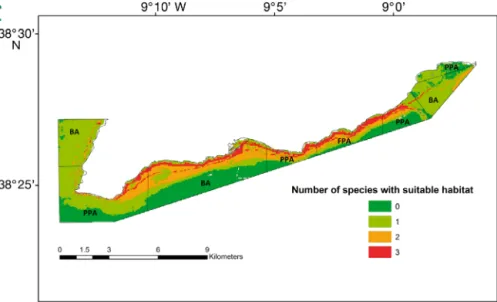
The area with suitable habitats for all of the studied species is limited to areas close to the coastline and where the coast is facing south (Fig. 6).
Vulnerability to fishing
The regulated zones where both the Senegalese sole and the white seabream are protected from fish-ing are larger than 25 km2 in total (fully protected
plus partially protected areas). For cuttlefish, the
area where it is fully protected from fisheries is the no-take (full-protection) area, which corresponds to approximately 4.2 km2. Although cuttlefish are also
protected in the first 200 m from the coastline in partially protected areas, these areas were not con -sidered, given their small size. Nevertheless, only a small proportion of these protected areas cor -responds to suitable habitats for these species (Table 2). In fact, of the entire LSMP, less than 8% presents suitable habitats for the 3 species, with the highest percentage being found in the fully protected area (Table 3). The vulnerability to fishing, consider-ing an individual’s home range centered in the mid-dle of the no-take area, was 0.0 for every species and home range considered (Fig. 7). In the western par-tial- protection area, the vulnerability to fishing was 0.0 for white seabream and Senegalese sole except when considering the maximum home range for Senegalese sole, where it reached a minimum of 0.05 (Fig. 7). D) Aspect E) Curvature 0.0 0.2 0.4 0.6 0.8 1.0 1 2 3 4 5 6 7 8 9 10 P ro b ab ilit y o f p re s e n c e Category 0.0 0.2 0.4 0.6 0.8 1.0 1 2 3 4 5 6 7 8 9 10 Category 0.0 0.2 0.4 0.6 0.8 1.0 1 2 3 4 5 6 7 8 9 10 Category 0.0 0.2 0.4 0.6 0.8 1.0 -1 .6 -1 .2 -0 .8 -0.5 -0.1 0. 3 0. 7 1. 1 1. 5 Probabi lity of presence Probabi lity of presence Curvature (1/100 m) 0.0 0.2 0.4 0.6 0.8 1.0 -1.6 -1.2 -0.8 -0.5 -0.1 0. 3 0. 7 1 .1 1. 5 Curvature (1/100 m) F) Slope 0.0 0.2 0.4 0.6 0.8 1.0 -1 .8 0.8 3.3 5.9 8.4 10 .9 1 3. 5 16 .0 18 .6 Slope angle (°) 0.0 0.2 0.4 0.6 0.8 1.0 -1 .8 0.8 3.3 5.9 8.4 1 0. 9 13 .5 16 .0 18 .6 Slope angle (°)
Sepia officinalis Solea senegalensis Diplodus sargus
Fig. 2 (continued)
Author
DISCUSSION
The results of the home range studies, together with the adequacy of the resulting models, allow us to draw important conclusions about the design suit-ability of the LSMP for cuttlefish, Senegalese sole and white seabream and the extent of protection offered by the MPA to these 3 species combined. Impor-tantly, this study goes a step further when compared with previous studies using home range areas only (e.g. Moffitt et al. 2009, Grüss et al. 2011) by combining this information with species distribution and in -direct habitat preference throughout the study area.
Model adequacy
The values of AUC obtained for the SDMs, when compared with the AUC value of the null models, are evidence that the final models obtained through Maxent are adequate and likely useful instruments (Swets 1988, Elith 2002) for the evaluation of the protection offered by MPA and the vulnerability to fishing. Additionally, a qualitative visual analysis of the resulting maps, made by local scientists and fishermen, also suggested that these models are helpful.
Although not frequently used in pre-vious SDM studies, correcting for sam-pling bias decreases the number of false presences and false absences (Syfert et al. 2013). As in other studies (e.g. Phillips & Dudík 2008, Radosavl-jevic & Anderson 2014), we show that species-specific tuning of model para -meters can im prove model performance. In addition, we used a totally inde-pendent test data set, which is consid-ered the most adequate approach to approximate optimal model complex-ity via tuning experiments (Phillips & Dudík 2008, Peterson et al. 2011). All of these measures are known to re duce model overfitting and im prove per-formance (Phillips & Dudík 2008, Radosavljevic & Anderson 2014). Nev-ertheless, the AUC and TSS values obtained are only marginally good, and some of the response curves (e.g. curvature) are complex, which could indicate model overfitting, probably because of data limitations (Elith & Graham 2009). Yet the AUC value itself should not be used as a guide to model utility, since it can be mis-leading (Lobo et al. 2008).
It could be argued that other potentially relevant input variables (e.g. hydro dynamics and prey distri-bution and abundance) could also prove useful to improve the predictive power of the spatial distribu-tion models of these species. However, informadistribu-tion on such variables was either absent or unavailable at adequate spatial scales for this area.
Importantly, the 6 variables that were selected to run the SDMs reflect various environmental factors known to influence marine species distributions. Fig. 3. (A) Habitat suitability map estimated with Maxent and (B,C) binary
suitability maps using (B) the lowest presence threshold and (C) the maximum sensitivity plus specificity threshold of Sepia officinalis in the Luiz Saldanha Marine Park during the months of November and December. Cross-hatched areas in (B,C) represent suitable habitats. BA = buffer area, PPA =
partial-protection area, FPA = full-partial-protection area
Author
The variable ‘habitat’ was used because marine spe-cies are known to prefer specific and sometimes distinct habitats throughout their life cycle. The variable ‘bathymetry’ is widely used as an indirect proxy for several proximal factors such as tempera-ture, light and pressure (Elith & Leathwick 2009b). The variable ‘aspect’ was se lected as a proxy for hydrodynamic variables, since in this specific case bottoms oriented to the southern and western quad-rants are more influenced by strong winds and high seas, whereas those facing the northern and eastern quadrants are more sheltered. The variables ‘slope’ and ‘curvature’ were also considered be cause these have been used as predictor variables for several marine species (Leathwick et al. 2008, Owens et al.
2012, Schmiing et al. 2013). The variable ‘distance to rock’ could be interpreted differently, de pending on the studied species. Adult white sea -bream, for instance, are known to prefer rocky bottom habitats (Abeca-sis et al. 2013b), and therefore ‘dis-tance to rock’ is likely to simply stand for distance to its preferred habitat. In the particular case of the cuttlefish, however, it can be in -terpreted as distance to spawning grounds, since this species prefers soft substrate but attaches its eggs to hard substrates like seaweeds, shells and debris (Ezzeddine-Najai 1997), and such substrates are also fre-quently found near shallow rocky bottoms. In fact, egg clutches were frequently ob served in the acoustic receivers’ mooring structures, partic-ularly in those located in vast sandy areas farthest away from rocky bot-toms (Abecasis et al. 2013a), where other hard substrates are absent or rare. These observations support the hypo thesis that cuttlefish use habitats closer to rocky bottoms during the spawning season because it is easier to find adequate substrates to attach their eggs. It also explains why the variables ‘distance to rock’ and ‘bath ymetry’ were the most impor-tant for the final cuttlefish’s SDM, especially considering that data col-lection took place during the migra-tion/ spawning months of November and December.
The response curves obtained for the predictor variables were, in some cases, very complex. Al -though this could indicate an unrealistic fit of the model, the AUC and TSS results ob tained show their adequacy. This is especially relevant because a low number of false negatives is highly desirable in the particular case of conservation spatial planning be -cause false negatives could lead to potentially suit-able areas being left out of management plans (Araújo & Guisan 2006).
The SDMs for Senegalese sole and white sea -bream were estimated with presence locations obtained throughout almost the entire year. There-fore, it is likely that the suitability maps represent an accurate picture for habitat selection of adults of Fig. 4. (A) Habitat suitability map estimated with Maxent and (B,C) binary
habitat suitability maps using (B) the lowest presence threshold and (C) the maximum sensitivity plus specificity threshold of Solea senegalensis in the Luiz Saldanha Marine Park. Cross-hatched areas in (B,C) represent suitable
habitats. Area abbreviations defined in Fig. 3
Author
both species in the LSMP. However, this was not the case for cuttlefish, for which presence data were only obtained for a shorter period of time (for more details, see Abecasis et al. 2013a). Considering that the cuttlefish is a migratory species that inhabits a wide range of habitats, it is highly probable that the distribution model obtained underestimates the true distribution for this species during its adult phase. Instead, the information provided by the model should be interpreted as an SDM for the cuttlefish’s
spawning period be cause presence data were
obtained from adults during this period (Abecasis et al. 2013a).
Habitat suitability
The suitability maps revealed that the LSMP area facing south contains the largest area of suitable habitats for all 3 species. The sheltering of this area from the dominant north winds and ocean swell has been put forward as one of the reasons for its high biodi-versity (Gonçalves et al. 2003).
Despite the fair to moderate TSS val-ues associated with the obtained SDMs, the results for white seabream might be slightly biased, given that the areas defined as suitable when using the MSST expanded farther away from rocky bottoms than anticipated, con-sidering the results of experimental fishing trials. Some bias related to less accurate positions used as training data may have occurred, and as a result, several sandy bottom areas relatively distant from rocky bottoms scored high suitability. Additionally, the method used to obtain the fishes’ fine-scale po-sitions limited the capability to distin-guish be tween a true position over rocky bottoms and an assumed position over sandy bottoms. The reason for this limitation is that the acoustic receivers were located in line with each other, parallel to the coast, and on sandy bot-toms. Consequently, nearly all locations were associated with sandy bottoms when, in fact, fish were likely roving over the nearby rocky bottoms within the de tection range. This possibility is supported by the inclusion of ‘distance to rock’ as the second most important variable for the white sea bream distri-bution model, confirming previous studies that demonstrated this species’ preference for rocky bot-toms, even though excursions to sandy bottoms may be frequent (Abecasis et al. 2013b). Regarding the Senegalese sole, the SDM model suggests that fine and medium sands are the habitats with the highest suitability, which is consistent with the results of habi-tat selection studies (Abecasis et al. 2014).
As in other studies of marine fish species (e.g. Leathwick et al. 2008, Lefkaditou et al. 2008), ‘ba-thymetry’ was the variable that most contributed to the distribution models. According to our models, the depth interval in which the white seabream and the Fig. 5. (A) Habitat suitability map estimated with Maxent and (B,C) binary
habitat suitability maps using (B) the lowest presence threshold and (C) the maximum sensitivity plus specificity threshold of Diplodus sargus in the Luiz Saldanha Marine Park. Cross-hatched areas in (B,C) represent suitable habitats.
Area abbreviations defined in Fig. 3
Author
Senegalese sole were more common is consistent with the results obtained during the experimental fishing (Cunha et al. 2011). For the cuttlefish, the model suggested that suitable habitats were limited to the interval between 0 and 40 m deep. However, this might not reflect the true bathymetric distri-bution of this species, which is known to occur at depths up to 200 m (Guerra 2006), particularly because the area monitored during the acoustic teleme-try campaigns was confined to shal-lower habitats because of the limited number of receivers available. More-over, the presence locations were ob-tained during a short period of time that overlapped the spawning season, during which time cuttlefish have been re ported to migrate into shallower wa-ters (Ezzeddine-Najai 1997, Gauvrit et al. 1997, Wang et al. 2003).
Protection
Our results demonstrate that the LSMP offers different levels of protec-tion, depending on species. This is not only the result of the different regula-tions applied to each of the LSMP’s zones (e.g. the fishery targeting cuttle-fish is only forbidden within the no-take zone, whereas the fisheries targeting Senegalese sole and white seabream are forbidden in both the no-take and partially protected zones) but also a consequence of the different move-ment patterns and home range areas re quired by each species.
Overall, the LSMP appears to provide full protection from fisheries to individ-uals of white seabream and Senegalese sole that have their home ranges cen-tered anywhere in the no-take area or in central areas of partial-protection zones. In fact, the results of a recent study suggest that the white seabream may already be benefiting from imple-mentation of the LSMP, given the in-crease in its abundance and biomass (Horta e Costa et al. 2013). For the Senegalese sole, the LSMP seems to Fig. 6. Overlap of the binary suitability maps that achieved the highest true
skill statistic for the study species (Sepia officinalis, Solea senegalensis and
Diplodus sargus). BA = buffer area, PPA = partial-protection area, FPA =
full-protection area
Variable S. officinalis S. senegalensis D. sargus
LPT MSST LPT MSST LPT MSST Avg. HR (km2) 1.26a 1.26a 1.19 1.19 0.65 0.65 FPA (km2) 4.2 4.2 25.3 25.3 25.3 25.3 FPSA (km2) 3.2 1.5 14.7 6.4 10.4 2.9 Minimum length HR (km) 0.9 0.9 0.9 0.9 0.9 0.9 Avg. length HR (km) 2.26 2.26 1.89 1.89 1.39 1.39 Maximum length HR (km) 3.5 3.5 2.8 2.8 3.4 3.4
aHome range areas based on minimum convex polygon
Table 2. Average home range area (Avg. HR), size of full-protection areas (FPA) and full-protection suitable areas (FPSA) for Sepia officinalis, Solea
senegalensis and Diplodus sargus. LPT indicates habitat suitability maps
based on the lowest presence threshold; MSST indicates habitat suitability maps based on maximum sensitivity plus specificity threshold. For S.
sene-galensis and D. sargus, the marine reserve area includes the full-protection
and partial-protection areas. For S. officinalis, the marine reserve area only includes the full-protection area
No. of Entire Full-protection Partial-protection Buffer species MPA (%) area (%) area (%) area (%) 0 29.47 22.94 31.54 29.03 1 44.29 26.19 44.64 46.77 2 18.85 28.27 16.76 19.03 3 7.39 22.60 7.07 5.17 Table 3. Percentage of suitable habitat for 0, 1, 2 and 3 of the study species (Sepia officinalis, Diplodus sargus and Solea senegalensis) in the entire
marine protected area (MPA) and in each protection level
Author
play an important role in the protection of local popu-lations, given the large size of suitable areas for this species located within areas where the species is fully protected. However, the effects of protection to this species are yet to be detected (Abecasis et al. 2014).
The cuttlefish, in contrast, appears to benefit less from protection, as our results indicate higher vulner-ability to fishing throughout the LSMP. Previous studies suggest that this species presents low site fidelity and undertakes large migrations (Wang et al. 2003, Abecasis et al. 2013a), which is consistent with the short periods of time in which tagged cuttlefish remained within the study area. Therefore, despite the protection provided by the no-take area to cuttle-fish, this result might be misleading, since this spe-cies presents no site fidelity.
This study focuses on adult individuals only. In fact, some life history stages of the study species are not common in the study area. Important factors such as larval dispersal, early life history periods and recruit-ment should be considered when overall MPA effi-ciency is assessed, especially when species persist-ence is considered. Nevertheless, this study provides
important information regarding the protection of commercially important fish species and how habitat suitability should be taken into account.
CONCLUSIONS
This study demonstrates that the combined use of home range areas and SDMs allows for an estimate of the increase in vulnerability to fishing as a function of the species’ habitat use and shape of the reserve units. It shows that such an increase will vary sub-stantially, depending on the species’ behaviour, and can be modulated by the distribution of their pre-ferred habitat patches within the reserve. This study differs from previous classical works analysing the implications of fish biotelemetry to spatial manage-ment by upscaling from individual telemetry data to the population scale of relevance for the assessment of MPA effectiveness and optimal design. Also, con-trary to most conceptual modeling MPA studies, our approach is driven by individual movement and habitat use data rather than by previously defined Fig. 7. Vulnerability to fishing for Sepia officinalis, Solea senegalensis and Diplodus sargus in the Luiz Saldanha Marine Park. The dotted line indicates vulnerability estimates considering the minimum home range, the black line indicates vulnerability considering the average home range and the dashed line indicates vulnerability considering the maximum home range. BA =
buffer area, PPA = partial-protection area, FPA = full-protection area
Author
behavioural patterns for the species and is thus a bet-ter representation of their behavioural patbet-terns and implications of reserve scenarios and vice versa.
This methodology can and should be used in iden-tifying multispecies MPA designs, whether this is done a priori or as part of an adaptive management strategy of MPAs. In the particular case of the LSMP, the levels of protection suggest that this MPA may provide adequate protection for the Senegalese sole and the white seabream if compliance is adequate, but this is not the case for the cuttlefish, given this species’ higher levels of exposure to fisheries and very low residency. Nevertheless, to determine the effectiveness of an MPA to achieve species persist-ence factors such as larval dispersal, fishing effort outside the MPA, recruitment parameters and mini-mum population size must also be considered. Acknowledgements. This research was partially supported
by the Foundation for Science and Technology (FCT) through indi vidual support to D.A. (SFRH/BD/46286/2008) and P.A. (Ciência 2008/POPH/QREN). Part of this study was funded by the Biomares LIFE project (LIFE06 NAT/333 P/ 000192). We are grateful to all of the Biomares LIFE re searchers and volunteers, who carried out the trammel net surveys, and to Vitor Henriques (IPMA) and colleagues, who provided the bathymetry and habitat mapping data.
LITERATURE CITED
Abecasis D (2013) Multispecies spatial dynamics under dif-ferent protection levels: an evaluation of the effects and optimal design of the Luiz Saldanha Marine Park. PhD thesis, Universidade do Algarve, Faro
Abecasis D, Bentes L, Coelho R, Correia C and others (2008) Ageing seabreams: a comparative study between scales and otoliths. Fish Res 89: 37−48
Abecasis D, Afonso P, O’Dor RK, Erzini K (2013a) Small MPAs do not protect cuttlefish (Sepia officinalis). Fish Res 147: 196−201
Abecasis D, Bentes L, Lino PG, Santos MN, Erzini K (2013b) Residency, movements and habitat use of adult white sea bream (Diplodus sargus) between natural and artificial reefs. Estuar Coast Shelf Sci 118: 80−85
Abecasis D, Afonso P, Erzini K (2014) Can small MPAs pro-tect local populations of a coastal flatfish, Solea
sene-galensis? Fish Manag Ecol 21: 175−185
Afonso P, Fontes J, Holland KN, Santos RS (2009) Multi-scale patterns of habitat use in a highly mobile reef fish, the white trevally Pseudocaranx dentex, and their implica-tions for marine reserve design. Mar Ecol Prog Ser 381: 273−286
Allouche O, Tsoar A, Kadmon R (2006) Assessing the accu-racy of species distribution models: prevalence, kappa and the true skill statistic (TSS). J Appl Ecol 43: 1223−1232 Araújo MB, Guisan A (2006) Five (or so) challenges for
spe-cies distribution modelling. J Biogeogr 33: 1677−1688 Batista MI, Teixeira CM, Cabral HN (2009) Catches of target
species and bycatches of an artisanal fishery: the case study of a trammel net fishery in the Portuguese coast.
Fish Res 100: 167−177
Bean WT, Stafford R, Brashares JS (2012) The effects of small sample size and sample bias on threshold selection and accuracy assessment of species distribution models. Ecography 35: 250−258
Cunha A, Erzini K, Serrão E, Gonçalves E and others (2011) Restoration and management of biodiversity in the mar-ine park site Arrábida-Espiche (PTCON0010). Biomares Project No. LIFE06 NAT/P/000192 final report, Centro de Ciências do Mar, Universidade do Algarve, Faro Elith J (2002) Quantitative methods for modeling species
habitat: comparative performance and an application to Australian plants. In: Ferson S, Burgman M (eds) Quanti-tative methods for conservation biology. Springer, New York, p 39−58
Elith J, Graham CH (2009) Do they? How do they? WHY do they differ? On finding reasons for differing performances of species distribution models. Ecography 32: 66−77 Elith J, Leathwick JR (2009a) The contribution of species
distribution modelling to conservation prioritization. In: Moilanen A, Wilson KA, Possingham HP (eds) Spatial conservation prioritization: quantitative methods & com-putational tools. Oxford University Press, Oxford, p 70−93 Elith J, Leathwick JR (2009b) Species distribution models:
ecological explanation and prediction across space and time. Annu Rev Ecol Evol Syst 40: 677−697
Elith J, Graham CH, Anderson RP, Dudík M and others (2006) Novel methods improve prediction of species’ distribu-tions from occurrence data. Ecography 29: 129−151 Elith J, Phillips SJ, Hastie T, Dudík M, Chee YE, Yates CJ
(2011) A statistical explanation of MaxEnt for ecologists. Divers Distrib 17: 43−57
Ezzeddine-Najai S (1997) Tagging of the cuttlefish, Sepia
officinalis L. (Cephalopoda: Decapoda), in the Gulf of Tunis. Sci Mar 61: 59−65
Gauvrit E, Goff RL, Daguzan J (1997) Reproductive cycle of the cuttlefish, Sepia officinalis (L.), in the northern part of the Bay of Biscay. J Molluscan Stud 63: 19−28
Glazer RA, Delgado GA (2006) Designing marine fishery reserves using passive acoustic telemetry. In: Taylor JC (ed) Emerging technologies for reef fisheries research and management. NOAA Professional Paper NMFS 5, Seattle, WA, p 26−37
Gonçalves EJ, Henriques M, Almada VC (2003) Use of a temperate reef-fish community to identify priorities in the establishment of a marine protected area. In: Beumer JP, Grant A, Smith DC (eds) Aquatic protected areas: What works best and how do we know? Proc World Con-gress on Aquatic Protected Areas, Cairns, Australia, August 2002, Australian Society for Fish Biology, Hobart, p 261−272
Grüss A, Kaplan DM, Guénette S, Roberts CM, Botsford LW (2011) Consequences of adult and juvenile movement for marine protected areas. Biol Conserv 144: 692−702 Guerra A (2006) Ecology of Sepia officinalis. Vie Milieu 56:
97−107
Guisan A, Thuiller W (2005) Predicting species distribution: offering more than simple habitat models. Ecol Lett 8: 993−1009
Guisan A, Zimmermann NE (2000) Predictive habitat distri-bution models in ecology. Ecol Modell 135: 147−186 Hernandez PA, Graham CH, Master LL, Albert DL (2006)
The effect of sample size and species characteristics on performance of different species distribution modeling methods. Ecography 29: 773−785
Author
Horta e Costa B, Erzini K, Caselle JE, Folhas H, Gonçalves EJ (2013) ‘Reserve effect’ within a temperate marine pro-tected area in the north-eastern Atlantic (Arrábida Mar-ine Park, Portugal). Mar Ecol Prog Ser 481: 11−24 Kaiser MJ (2011) Uncertainty demands an adaptive
man-agement approach to the use of marine protected areas as management tools. In: Ommer RE, Perry RI, Cochrane K, Cury P (eds) World fisheries: a social-ecological analysis. Wiley-Blackwell, Oxford, p 351−358
Landis JR, Koch GG (1977) The measurement of observer agreement for categorical data. Biometrics 33: 159−174 Le Goff R, Daguzan J (1991) Growth and life-cycles of the
cuttlefish Sepia officinalis L (Mollusca, Cephalopoda) in South Brittany (France). Bull Mar Sci 49: 341−348 Le Quesne WJF, Codling EA (2009) Managing mobile species
with MPAs: the effects of mobility, larval dispersal, and fishing mortality on closure size. ICES J Mar Sci 66: 122−131 Leathwick J, Moilanen A, Francis M, Elith J and others (2008) Novel methods for the design and evaluation of marine protected areas in offshore waters. Conserv Lett 1: 91−102 Lefkaditou E, Politou CY, Palialexis A, Dokos J, Cosmopou-los P, Valavanis V (2008) Influences of environmental variability on the population structure and distribution patterns of the shortfin squid Illex coindetii (Cepha -lopoda: Ommastrephidae) in the eastern Ionian Sea. Hydrobiologia 612: 71−90
Lester SE, Halpern BS, Grorud-Colvert K, Lubchenco J and others (2009) Biological effects within no-take marine reserves: a global synthesis. Mar Ecol Prog Ser 384: 33−46 Liu C, Berry PM, Dawson TP, Pearson RG (2005) Selecting thresholds of occurrence in the prediction of species distributions. Ecography 28: 385−393
Lobo JM, Jiménez-Valverde A, Real R (2008) AUC: a mis-leading measure of the performance of predictive distri-bution models. Glob Ecol Biogeogr 17: 145−151
Meynard CN, Kaplan DM (2012) The effect of a gradual response to the environment on species distribution modeling performance. Ecography 35: 499−509
Moffitt EA, Botsford LW, Kaplan DM, O’Farrell MR (2009) Marine reserve networks for species that move within a home range. Ecol Appl 19: 1835−1847
Navarro-Cerrillo RM, Bermejo JE, Hernández-Clemente R (2011) Evaluating models to assess the distri-bution of Buxus balearica in southern Spain. Appl Veg Sci 14: 256−267
Newbold T (2009) The value of species distribution models as a tool for conservation and ecology in Egypt and Britain. PhD thesis, University of Nottingham
Owens H, Bentley A, Peterson A (2012) Predicting suitable environments and potential occurrences for coelacanths (Latimeria spp.). Biodivers Conserv 21: 577−587
Pearson RG, Raxworthy CJ, Nakamura M, Townsend Peter-son A (2007) Predicting species distributions from small numbers of occurrence records: a test case using cryptic geckos in Madagascar. J Biogeogr 34: 102−117
Peterson AT, Soberón J, Pearson RG, Anderson RP, Martínez-Meyer E, Nakamura M, Araújo MB (2011) Ecological niches and geographic distributions (MPB-49). Princeton University Press, Princeton, NJ
Phillips SJ, Dudík M (2008) Modeling of species distribu-tions with Maxent: new extensions and a comprehensive evaluation. Ecography 31: 161−175
Phillips SJ, Anderson RP, Schapire RE (2006) Maximum entropy modeling of species geographic distributions. Ecol Modell 190: 231−259
Phillips SJ, Dudik M, Elith J, Graham CH, Lehmann A, Leathwick J, Simon F (2009) Sample selection bias and presence-only distribution models: implications for background and pseudo-absence data. Ecol Appl 19: 181−197
Quéro JC, Desoutter M, Lagardère F (1986) Soleidae. In: Whitehead PJ, Bauchot ML, Hureau JC, Nielsen J, Tor-tonese E (eds) Fishes of the north-eastern Atlantic and the Mediterranean. UNESCO, Paris, p 1308–1328 Radosavljevic A, Anderson RP (2014) Making better Maxent
models of species distributions: complexity, overfitting and evaluation. J Biogeogr 41: 629−643
Raes N, ter Steege H (2007) A null-model for significance testing of presence-only species distribution models. Ecography 30: 727−736
Reynolds TD, Laundre JW (1990) Time intervals for estimat-ing pronghorn and coyote home ranges and daily move-ments. J Wildl Manag 54: 316−322
Rodda GH, Jarnevich CS, Reed RN (2011) Challenges in identifying sites climatically matched to the native ranges of animal invaders. PLoS ONE 6: e14670
Schmiing M, Afonso P, Tempera F, Santos RS (2013) Predic-tive habitat modelling of reef fishes with contrasting trophic ecologies. Mar Ecol Prog Ser 474: 201−216 Simpfendorfer CA, Heupel MR, Hueter RE (2002)
Estima-tion of short-term centers of activity from an array of omnidirectional hydrophones and its use in studying animal movements. Can J Fish Aquat Sci 59: 23−32 Swets JA (1988) Measuring the accuracy of diagnostic
systems. Science 240: 1285−1293
Syfert MM, Smith MJ, Coomes DA (2013) The effects of sampling bias and model complexity on the predictive performance of MaxEnt species distribution models. PLoS ONE 8: e55158
Teixeira CM, Cabral HN (2010) Comparative analysis of the diet, growth and reproduction of the soles, Solea solea and Solea senegalensis, occurring in sympatry along the Portuguese coast. J Mar Biol Assoc UK 90: 995−1003 Thorn JS, Nijman V, Smith D, Nekaris KAI (2009) Ecological
niche modelling as a technique for assessing threats and setting conservation priorities for Asian slow lorises (Pri-mates: Nycticebus). Divers Distrib 15: 289−298
Veiga P, Ribeiro J, Gonçalves JMS, Erzini K (2010) Quantify-ing recreational shore anglQuantify-ing catch and harvest in southern Portugal (north-east Atlantic Ocean): implica-tions for conservation and integrated fisheries manage-ment. J Fish Biol 76: 2216−2237
Walters CJ, Hilborn R, Parrish R (2007) An equilibrium model for predicting the efficacy of marine protected areas in coastal environments. Can J Fish Aquat Sci 64: 1009−1018
Wang JJ, Pierce GJ, Boyle PR, Denis V, Robin JP, Bellido JM (2003) Spatial and temporal patterns of cuttlefish (Sepia
officinalis) abundance and environmental influences — a
case study using trawl fishery data in French Atlantic coastal, English Channel, and adjacent waters. ICES J Mar Sci 60: 1149−1158
Warren DL, Seifert SN (2011) Ecological niche modeling in Maxent: the importance of model complexity and the performance of model selection criteria. Ecol Appl 21: 335−342
Yackulic CB, Chandler R, Zipkin EF, Royle JA, Nichols JD, Campbell Grant EH, Veran S (2013) Presence-only mod-elling using MAXENT: When can we trust the infer-ences? Methods Ecol Evol 4: 236−243
Editorial responsibility: Romuald Lipcius, Gloucester Point, Virginia, USA
Submitted: October 15, 2013; Accepted: August 5, 2014 Proofs received from author(s): September 29, 2014