Credit ratings and stock markets : an event-study approach

Cred

it

Rat

ings

and

Stock

Markets:

An Event-Study Approach

Tomás

Trovão

D

issertat

ion

wr

itten

under

the

superv

is

ion

o

f

Dagf

inn

R

ime

D

issertat

ion

subm

itted

in

part

ia

l

fu

l

f

i

lment

o

f

requ

irements

for

the

MSc

in

F

inance

,

at

Un

ivers

idade

Cató

l

ica

Portuguesa

and

for

the

MSc

in

F

inance

,

at

Acknowledgements

This thesis, developed throughout the academic year of 2016/17 in Oslo, Norway, represents the end of my Double Degree Master program between Católica-Lisbon SBE and BI Norwegian Business School.

I would like to thank my supervisor, professor Dagfinn Rime, as his guidance and feedback were absolutely crucial during the development of this thesis.

Even though he did not help directly in the development of this thesis, I would also like to thank professor José Faias. Not only was the knowledge provided in Empirical Finance of the outmost importance for this thesis, Faias et al. (2012) served as the guideline for it.

On a personal note I would like to thank my family, especially my parents, for not only giving me the opportunity to study in Norway but also for their constant support and love throughout my life.

I would also like to thank my friends. Without their support and joy neither this thesis nor my life would be the same. A special mention must be given to Rafa, for always setting the tone academically.

Last, but certainly not least, I would like to thank Mariana for convincing me to come to Norway. This was a special year, spent with a special person.

Abstract

The impact of sovereign credit downgrades on financial markets was deeply scrutinized on the aftermath of the 2008 financial crisis, especially in Southern Europe. The purpose of this thesis is to analyze the impact of sovereign credit rating downgrades both on National and Foreign stock markets through an Event-Study methodology. The main focus is the impact generated by S&P and Moody’s downgrades on market indexes from advanced economies throughout the world. This approach was taken to compare the impact felt by the downgraded countries with the impact on other countries belonging to that same region. Even though I find little evidence of national impact outside Europe, where the abnormal returns range from -0,03% to -0,2% on the event date, my analysis suggests that there is evidence of spillover effects throughout the developed world, as one of the models used finds significant negative abnormal returns on the event date in 2 out of the 3 estimation windows considered, the third being marginally insignificant. Regardless of the model the spillover creates abnormal returns that go from 0% to -0,4%.

Abstracto

O impacto dos downgrades da dívida soberana nos mercados financeiros foi profundamente escrutinado depois da crise de 2008, especialmente no Sul da Europa. O propósito desta tese é analisar o impacto do downgrade do rating da dívida soberana nos mercados de acções nacionais e internacionais através da metodologia Event-Study. O foco principal é o impacto gerado por downgrades da S&P e da Moody’s nos índices de mercado de várias economias desenvolvidas. Esta abordagem foi seguida de modo a comparar o impacto sentido pelos países que sofreram um downgrade com o impacto gerado noutros países da região. Ainda que encontre poucas evidências de um impacto nacional fora da Europa, onde os retornos anormais variam entre -0,03% e -0,2% no dia do evento, a minha análise sugere que existem evidências de efeitos de spillover nas várias economias analisadas, dado que um dos modelos usados encontrou retornos anormais significantes em 2 das 3 janelas usadas, sendo que a 3ª foi marginalmente insignificante. Ignorando os modelos usados, os retornos anormais no dia do evento variam entre 0% e -0,4%.

CONTENTS Acknowledgements I Abstract II Abstracto III Academic Content IV 1. Introduction 7 1.1. Introduction 7 1.2. Research Questions 9 1.3. Thesis Outline 9 2. Literature Review 9

2.1. Credit Rating Agencies 9

2.2. National Impact 12 2.3. International Impact 13 3. Event-Study Methodology 15 3.1. Event Date 15 3.2. Estimation Window 15 3.3. Event Window 16 3.4. Abnormal Returns 17 4. Data 20

4.1. Countries and Indexes 20

4.2. Market Index 21

4.3. Time Period 22

4.4. Credit Rating Agencies 22

4.5. Announcement Dates 22

5. Result Analysis 23

5.1. 120 day Estimation Window 23

5.2. 60 day Estimation Window 24

5.3. 20 day Estimation Window 24

6. Conclusions 27

References V

1. Introduction

1.1. Introduction

On the 5th _{of July of 2011 Portugal’s long-term credit rating was downgraded to Ba2 in Moody’s}

rating scale, signaling that the country’s debt was not “Investment Grade” for the first time in the

21st _{century. By the 5}th _{of August, the Portuguese Stock Index (PSI20) had lost 15% of its initial}

value (on the 5th _{of July), in that same period the Italian FTMIB and the Spanish IBEX35 lost,}

respectively, 21% and 16% of their initial value, even though the national credit ratings stayed the same.

O’Rourke (2002) shows that the relative weight of world exports on world GDP has increased from 5,5% to 17,2% between 1950 and 1998. He argues that such evolution is a consequence of the economic phenomenon known as Globalization, which Larsson (2001) defines as the increasing ease with which somebody on one side of the world can interact, to mutual benefit, with somebody on the other side of the world. Even though economists often focused on the benefits of increasing integration, with financial experts frequently emphasizing the benefits of international risk diversification (Wolf and Drezner (2005), McNicoll (2004)), the risks of growing integration were often overlooked until 2008. In this year the American sub-prime crisis, whose predictive signs had arisen in precedent years, instigated the freezing of the American Money Market, since lenders did not know the extent of the borrowers’ exposure to the housing market (Krishnamurthy (2010)). European financial institutions, especially banks, not only had some of their short term debt denominated in American dollars, which they were not able to rollover then, but a growing part of their investments were done in American mortgage related securities, which were losing value every day (Baba et al. (2009)). As such, the contagion effects from the downturn in the American economy were soon felt across Europe. In this climate of high risk-aversion, the sustainability of the large piles of sovereign debt accumulated by some European countries over the previous years were soon to be questioned.

Credit ratings provide market participants with (new) information regarding the borrower’s ability to repay the loan. In this period of uncertainty, the aftermath of the 2008 crisis, investors relied on the analysis of the rating agencies to better assess the credit worthiness of the most vulnerable countries. However, as will be presented in detail afterwards, a stylized fact concerning credit rating agencies has emerged through time: their ratings are procyclical, upgrades are more

likely to occur in economic expansions whereas downgrades are more likely to occur in periods of economic recession. In the case of firms such downgrades are felt in negative stock returns and

increasing bond yields1. Downgrades of sovereign debt on the other hand have real effects on

national stock markets: Brooks et al. (2004), Hooper et al. (2008), Pukthuanthong-Le et al. (2007) Mateev (2014) and Bissoondoyal-Bheenick and Brooks (2008) all find significant negative impacts on stock markets when the country’s rating is downgraded for example. Moreover, some studies such as Partnoy (1999) have challenged the premise that new information is conveyed to the market. If we combine these two ideas with the Home Bias hypothesis (national investors tend to invest more at home than they should), we can see the importance of such event for the country being downgraded. Even though, one must say, such hypothesis will be a barrier for the dispersion effects analyzed afterwards, as it will act as an insulation mechanism for the neighbor countries.

An issue that has not been studied in detail is how stock market crashes originated by sovereign rating downgrades spill over into other stock markets. If, as some of the literature suggests, stock markets are contagion bridges across countries, (Forbes and Rigobon (1999), Calvo and Reinhart (1996)), then not only were the countries being negatively reviewed vulnerable, but other countries were potentially exposed as well. Such exposure was, in the case of Europe, amplified by the common currency, the Euro, since economic and financial shocks spread faster and stronger in currency unions (Rose and Engel (2000)). The case of the downgrade of the Portuguese debt presented in the first paragraph of this introduction, and the effects it had across the three countries identified, seems to suggest that European countries were, and still might be, vulnerable to third party’s credit downgrades.

In order to better manage future international economic and financial shocks, and accordingly avoid consequences that are not inevitable, it is necessary to study how shocks were transmitted and the effects they produced in the past. Moreover, the study of the mechanisms of shock transmission might lead to a better analysis of systematic risk, which can increase the benefits of international portfolio diversification for investors, a benefit that will be visible in the economy. As previously stated, there is little literature concerning the spillover effects of credit ratings between developed nations. Ferreira and Gama (2007), Afonso et al. (2014) and Faias et al. (2012) seem to be the exceptions.

1Barron et al. (1997), Cornell et al. (1989), Ederington and Goh (1998), Glascock et al. (1987), Goh

and Ederington (1993), Griffin and Sanvincente (1982), Holthausen and Leftwich (1986), Hsueh and Liu (1992); Impson et al. (1992), Liu and Smith (1999), Matolcsy and Lianto (1995), Wansley et al. (1992), Zaima and McCarhty (1988)

1.2.Research Questions

With the purpose of understanding the effects of sovereign credit downgrades on both national and international stock markets this thesis will focus on downgrades by the two largest credit rating agencies, Moody’s and Standard & Poor’s (S&P), on countries from the most financially developed regions in the world (Europe, North America, East Asia and Oceania) in the period between 2009 and 2015. More precisely, the main goal will be to answer the following questions:

(1) How did credit downgrades affect national stock markets?

(2) How did the neighboring countries’ stock markets react to such event?

1.3.Thesis Outline

This thesis is divided in six sections. In the present section, section 1, the topic of the thesis is introduced and its’ goals made clear. Section 2 begins with an introduction of the Credit Rating industry and the stylized facts related to this industry; it is followed by a review of existing literature regarding the impact of credit rating downgrades on national financial markets (stocks, bonds and currency); and concluded with the literature that concerns the spillover to foreign stock markets. In section 3 the Event-Study methodology is introduced and analyzed in detail, especially the test statistics that can be applied to such methodology. Section 4 concerns the data which will be used to answer the questions presented before, the selection process of such data is presented as well as a detailed analysis of the data. Section 5 will contain the results obtained by applying the methodology and the analysis of the same. Section 6 concludes and suggests some areas for further research.

2. Literature Review

2.1. Credit Rating Agencies

In 1909, John Moody published the first publicly available bond rating, focused on railroad companies’ bonds, a sector that had seen an immense increase in the default rates during the 1870s (Giesecke et al. (2011)). By 1913 his analysis had expanded into industrial and utilities’ related companies. White (2010) states that his success attracted more companies into the industry: in 1916

Poor’s Publishing Company started issuing ratings, Standard Statistics Company followed in 1922 and Fitch Publishing Company entered the market in 1924.

The purpose of Moody’s analysis was to evaluate the borrower’s credit worthiness, that is, their ability to repay their debt. By doing this the agency decreased the information asymmetry between the lender and the borrower. This reduction allowed, and still does, for a better screening of the borrowers and hence a more appropriate use of available resources, that not only creates economic growth but decreases the likelihood of a financial crisis (Bernanke and Blinder (1992)). To obtain this analysis investors would pay for it. However the industry changed in the 1970s, mainly due to two factors (White (2010)). Firstly the introduction of photocopy machines in everyday life made it impossible for credit rating agencies to continue operating their business model, as investors could buy one single manual an photocopy it among themselves. As such the companies switched from an “investor pay” based model to an “issuer pay” based model. This change has been controversial, as now issuers pay for ratings, an action that might distort the agencies’ incentives to criticize the issuer’s ability to repay. Secondly the bankruptcy of Penn-Central Railroad in 1970 shocked the market. This shock made both bond issuers and rating agencies aware of the importance of credit ratings (Fridson (1999)): issuers wanted to assure investors they would not default and rating agencies realized they were crucial for the market to operate properly. In fact, in 1999, New York Times columnist Thomas Friedman wrote:

“There are two superpowers in the world (…) there’s the United States and there’s Moody’s (…)

it’s not clear who’s more powerful”.

The impact of corporate downgrades on the firm’s debt and equity has been studied in depth, and two particular stylized facts have surged. On the one hand, credit rating upgrades appear to have no impact on either debt or equity, that is, there is no positive abnormal return associated with the

firm’s equity or any abnormal negative impact on the firm’s debt yield2. On the other hand, credit

rating downgrades appear to have a significant negative impact on both equity and debt, the former

presents abnormal negative returns whereas the latter sees its’ yield increase abnormally2_.

2Barron et al. (1997), Cornell et al. (1989), Ederington and Goh (1998), Glascock et al. (1987), Goh

and Ederington (1993), Griffin and Sanvincente (1982), Holthausen and Leftwich (1986), Hsueh and Liu (1992); Impson et al. (1992), Liu and Smith (1999), Matolcsy and Lianto (1995), Wansley et al. (1992), Zaima and McCarhty (1988)

More recently, a third stylized fact has emerged: procyclicality. According to recent research credit ratings tend to follow economic cycles: upgrades occur more often in economic expansions whereas downgrades are more common in economic downturns (Cesaroni (2015), Bangia et al. (2002), Loffler (2004), Kiff et al. (2013), Valles (2006)). These authors claim that this happens because during periods of crisis the value of firms’ tends to decrease, increasing the relative size of debt, which makes it more difficult to repay. This new piece of evidence has created further discussion about the role of credit rating agencies in financial markets, as they might deepen the cycles instead of smoothing them, which might widen the impact on firm value.

Despite the importance of ratings in capital markets and the non-disclosure of the rating determination methodology, several academic papers have, to some extent, successfully deduced how credit ratings are determined (Cantor and Packer (1994), Afonso (2003), Afonso et al. (2011)). Cantor and Packer (1994), one of the first attempts to replicate the models used by the agencies,

were able to attain an R2 _{of 92% using just 7 economic variables to predict sovereign rating,}

whereas the most recent of these studies, Afonso et al. (2011) develops a model that accurately predicts the sovereign rating in over 75% of the cases. Furthermore model’s such as the Altman’s Z-Score can be used to predict the default probability of companies without resorting to rating agencies. Even though the models presented are not perfect substitutes of the models used by the credit rating agencies, they have significant predictive power. Accordingly some authors have challenged the premise that these agencies provide new information to the market. Partnoy (1999) argues that agencies have not only survived, but also thrived, not due to the content of their analysis, but because they have become a crucial element in financial regulations of developed countries. To back such argument he looks into SEC’s market regulations, central banks’ bond purchase regulations. Moreover he claims that the content of the agencies’ analysis has been increasingly void of statistical proof and increasingly filled with subjective analysis, which he proves by looking at how credit default swaps’ premiums float over time, even though the underlying credit rating does not change.

If Partnoy (1999) is correct one should expect the Cumulative Abnormal Returns from the analysis to be close to zero sometime after the downgrade is announced since, according to the semi-strong Efficient Market Hypothesis proposed by Eugene Fama, new information would permanently change the value of the assets in question.

2.2. National Impact

As presented before the impact of credit downgrades at a firm level has been heavily studied. Nonetheless extensive research has been done on the impact of sovereign downgrades on national credit and stock markets. The studies presented below were all completed using the Event-Study methodology In the next chapter this methodology is thoroughly explained.

Brooks et al. (2004) study the effect of credit rating changes by Moody’s, S&P, Fitch and Thompson on national stock markets between 1973 and 2000. In accordance with the previously presented stylized facts they find that upgrades have no impact on the stock markets while downgrades cause significant negative abnormal returns on the stock markets. Moreover, they find that different agencies have different power, S&P being the agency that most affects the stock market. Finally such effect is lasting, that is, new information is conveyed to the market, altering the value of the securities analyzed.

Hooper et al. (2008) studies the impact of credit rating changes by Moody’s, S&P and Fitch on both the national stock market and the national currency for the period between 1995 and 2003. They find that both downgrades and upgrades affect significantly stock and foreign exchange markets, even though the strength of such impact is much higher in the case of downgrades. They conclude that an upgrade (downgrade) has a significant positive (negative) impact on stock markets that is also visible through lower (higher) stock volatility. Furthermore, in accordance with Brooks et al. (2004), they find that rating changes provide new information to the stock market, as the cumulative abnormal returns tend to persist over time. Nonetheless, the presence of abnormal returns prior to the announcement date seems to suggest that even though new information is provided to investors, they already expect it to some extent. Finally Hooper et al. (2008) finds no evidence that emerging economies are more exposed to rating changes than developed economies.

Pukthuanthong-Le et al. (2007) study the impact of credit rating changes by S&P on both the national stock and bond markets during the 90s. They find that downgrades have significant impacts on both markets whereas upgrades only affect bond markets through a decrease in the companies’ yields. They also find that high inflation, large budget deficits and large sovereign debt increase the magnitude of the downgrade effects. They conclude that emerging economies are, therefore, more vulnerable to rating changes than developed economies. However, contagion effects across classes are more visible in the case of economies where there is low inflation, low sovereign debt and high

liquidity. Hence, they determine that contagion effects across classes are more likely in developed economies rather than on emerging ones.

Bissoondoyal-Bheenick and Brooks (2008) use four different approaches to model stock returns in order to capture the impact of credit rating changes by S&P between 1975 and 2007. In two of these models, the quadratic market model and the higher order downside model, they find that both rating downgrades and upgrades have significant (negative and positive, respectively) impacts on national stock markets, even though the impact of downgrades is larger. Regarding the other two models used, the market model and the regular downside model, their results suggest that only downgrades impact (negatively) national stock markets.

Mateev (2012) studies the impact of rating changes by Moody’s, S&P and Fitch on both bond and stock markets in Eastern European countries in the period between 1998 and 2007. The author finds that only rating downgrades affected significantly these markets, through higher yields and lower returns, respectively. Moreover the author finds that downgrades (upgrades) are more likely during economic recessions (expansions), a discovery in line with the rating procyclicality theory previously mentioned.

With all this in mind one should therefore expect the national stock market of the downgraded country to suffer a significant decrease in value, even though there is room for mixed expectations regarding the duration of such decrease, as there have been contrary conclusions concerning the information given to the market (new vs already available). Such decrease will be amplified by the deep economic recession felt across parts of Europe during the period in question. In other words, in such context credit rating downgrades are only another factor depressing the stock markets.

2.3. International Impact

While the two previous impacts have been studied in detail (own firm and own country) the impact of rating changes of one country on another country has been somehow overlooked. Still, after the European sovereign debt crisis this issue has captured more interest among the academic community and more research has started to be developed on the topic.

Using data ranging from 1989 to 2003 Ferreira and Gama (2007) study how credit rating changes by S&P spillover from one country’s stock market to a foreign one in a cross-sectional way. They

find that only downgrades create an impact strong enough to spillover to other countries’ stock market, since upgrades have no effect on national stock markets in the first place. Additionally, such impact is inversely related to the distance between countries, a conclusion in line with previous economic theories such as the Gravity Equation proposed by Jan Tinbergen, that asserts that countries that are geographically closer to each other will be more connected economically. They also conclude that emerging economies are in fact more exposed to spillovers (bigger stock crash), and that the larger the country being downgraded the more likely it is for the spillover effects to be felt in other countries.

Afonso et al. (2014) investigates the connection between credit rating changes by S&P, Moody’s and Fitch in one European country and financial markets’ volatility in other European countries. They split these countries in two groups: financially stable countries (UK, Germany, etc.) and financially unstable countries (Portugal, Greece, etc.) and use an event-study methodology to capture abnormal volatility. Such separation is crucial since their data ranges from 1995 to 2011, capturing the European sovereign debt crisis. They find that only downgrades in a country affect volatility in others, increasing volatility in both the bond and stock market. Such impact is enhanced when the downgrade concerns a financially unstable country. Taking into account the studies presented before, where downgrades are believed to have a negative impact on national stocks, bonds and even currency, one can infer that downgrades will reduce the prices of bonds and stocks in countries other than the ones being downgraded, a finding in line with Ferreira et al. (2007).

Faias et al. (2012) studies the impact of credit downgrades by S&P not only on national stock markets but on other European stock markets for the period between 2008 and 2012. Using an event-study methodology they ascertain that both national and foreign stock markets significantly underperform, even though foreign stock markets’ underperformance is less pronounced when compared to the evolution observed in domestic markets. Afterwards, the abnormal returns registered in the foreign countries are regressed in a set of variables which includes a dummy variable that equals 1 if another country was downgraded. They find that such dummy variable is in fact significantly negative, meaning that there is evidence of spillover effects accross the European markets.

Accordingly, it is expectable that the other countries’ stock markets also underperform, but in a less pronounced way than the markets’ being downgraded. Moreover, the distance between those

countries should help amplify those effects, since all countries are geographically close to each other.

3. Event-Study Methodology

In order to capture the effect of rating downgrades on the stock markets this thesis will adapt the methodology proposed by Mackinlay (1997), applying it to market indexes rather than to individual stocks. The following section explains the methodology proposed and my application.

3.1. Event Date

The event date corresponds to the period in time where a certain action or announcement is made known to the market. In this thesis the event date will correspond to the date of the rating downgrade announcement by either Moody’s or S&P.

3.2. Estimation Window

In order to obtain the impact of the rating change on market returns one must first know what the returns would have been without that very impact. To do this we must model the index’s returns. In event-study related literature three types of models are widely used for stock analysis: the market model, factor models (such as the famous three Fama-French factors) and the constant mean return model. For the purpose of this thesis I will use the market model, since this was the model used in Mackinlay (1997), which, despite its simplicity, attained robust results.

In the market model, stock returns’ sources are divided into 2 components: firm specific returns, captured by α, and market originated returns, captured by β, which comprises the stock’s responsiveness to market movements:

𝑅_𝑖,𝑡 = 𝛼 + 𝛽 ∗ 𝑅_𝑚,𝑡+ 𝜀_𝑖,𝑡

As stated before, I will work with market indexes. As such, α will comprise the index’s individual movement, the part of the total return which cannot be explained by market movements, and β will capture the index’s response to market movements. Even though it seems somewhat redundant to check the market index’s response to movements in the market itself, it is easier to understand my idea if we consider the national market index as a portfolio composed only of national stocks, and the market portfolio as a global index. As such β will measure the national

portfolio’s response to movements in the world market, which is affected by countless other international factors.

It is important to mention that the model assumes that the error term ε has zero mean and constant variance. The failure of such assumption might lead to biased estimators. Nonetheless the widespread use of such model suggests that the failure of these assumptions is not a relevant issue. Accordingly the OLS estimation method will be used to obtain the parameters required.

The estimation window comprises the period prior to the event date which is used to obtain the parameters required by the model chosen, in my case the market model’s Beta and Alpha. In my first approach I will use the daily stock returns from the 120 days prior to the beginning of the event window. On the one hand the use of daily data enables me to capture in a clearer way the impact of the rating change, as more infrequent data would be more likely to contain impacts from other sources (noise). On the other hand 120 days, approximately 6 trading months, enables me to capture the typical behavior of the stock, especially regarding its’ relationship with the global market. To check if results are robust to different time spans an additional second and third approach, with Estimation Windows of 60 and 20 days respectively, will be developed. Even though smaller time spans encompass a smaller estimation sample, they also encompass less noise. Accordingly it will be interesting to see which of these offsetting effects dominates the quality of the model.

3.3. Event Window

The event window corresponds to the time period where the effects of the event being studied are felt by the securities being analyzed. Even though the rating downgrade announcement occurs at, say, day t my event window will begin prior to it, at day t-15, as credit rating announcements are known in advance, which might lead to speculation that in turn might affect the returns of the stocks prior to the event date (Hooper at al. (2008)). The event window will contain, at first, the 3 trading weeks (15 trading days) prior and after the announcement, encompassing a total 30 day period. Once again, to check for result robustness, the event window on my second and third approaches will be altered to 10 and 5 days after and prior the event.

Having defined the estimation window, the event date and the event window a figure can be drawn to better explain the methodology:

In the primary case T0 begins 120 days prior to T1. This period corresponds to the estimation

window which will be used to obtain the market model’s parameters. From T1 to T2, the period

comprising the 30 day event window in this case, the abnormal returns will be calculated. Even though Mackinlay (1997) proposes a third window, the Post-Event Window, to increase the robustness of the parameters estimated, it will not be used for the purpose of this thesis, as most of the research conducted using this methodology obtains robust estimators using the Estimation Window alone.

3.4. Abnormal Returns

The abnormal return corresponds to the part of the actual stock return which cannot be explained by the model used. In other words it is the difference between the actual return and the expected one:

𝐴𝑅_𝑖,𝑡 = 𝑅_𝑖,𝑡− (𝛼 + 𝛽 ∗ 𝑅_𝑚,𝑡)

Under the hypothesis that the event has no effect on the returns then the abnormal returns follow a normal distribution:

𝐴𝑅𝑖,𝑡~𝑁(0, 𝜎𝑖,𝑡2)

The abnormal return’s variance can be defined as: 𝜎_𝑖,𝑡2 _{= 𝜎} 𝜀2𝑖+ 1 𝑇₁− 𝑇₀(1 + [ 𝑅𝑚,𝑡− 𝜇̂𝑚 𝜎̂_𝑚 ] 2 )

As it is visible above, the variance can be divided into two parts. The first component comes from the variance of the market model residuals, ε, while the second component stems from the measurement error when obtaining the Beta and Alpha parameters for the market model. The

parameters µm and σm refer to the market’s sample average and variance, respectively. Mackinlay

(1997) argues that if the estimation window (T1-T0) is large enough the measurement error

component can be ignored. Assuming the estimation windows of 120, 60 and 20 days are large enough, then the variance becomes:

𝜎_𝑖,𝑡2 _{= 𝜎} 𝜀𝑖

2

To make result analysis simpler it is usual to aggregate abnormal returns into average abnormal returns. In our case this average will simply be the average of the abnormal returns of the different indexes of the sample in the same period in time, that is:

𝐴𝑅𝑡 = ∑ 𝐴𝑅̂𝑖,𝑡

𝑁

𝑖=1

After calculating the average abnormal returns Mackinlay (1997) suggests calculating the cumulative average abnormal returns. Such returns are the cumulative average of the previously calculated abnormal returns. For a single index:

𝐶𝐴𝑅

̂_{𝑖(𝑇1, 𝑇2) =} 1

𝑁∗ ∑ 𝐴𝑅̂𝑖,𝑡

𝑇2

𝑡=𝑇1

For the entire sample of indexes the cumulative average of abnormal returns is then: 𝐶𝐴𝑅(𝑇₁, 𝑇₂) =_𝑁1 ∗ ∑ 𝐶𝐴𝑅̂_𝑖(𝑇₁, 𝑇₂)

𝑁

𝑖=1

To test the significance of the average abnormal returns we must calculate their average and variance:

𝐴𝑅_𝑡 = 1

𝑁∗ ∑ 𝐴𝑅̂𝑖,𝑡

𝑁

𝑉𝑎𝑟(𝐴𝑅_𝑡) = 1

𝑁2∗ ∑ 𝜎𝜀2𝑖

𝑁

𝑖=1

As such under the null hypothesis that there is no impact, that is, the sovereign credit rating downgrade has no impact on the stock markets, the test statistic z follows asymptotically a standard Normal distribution:

𝑧 = 𝐴𝑅𝑡

√𝑉𝑎𝑟(𝐴𝑅_𝑡)

Regarding the cumulative average abnormal returns the average and variance is:

𝐶𝐴𝑅(𝑇1, 𝑇2) = ∑ 𝐴𝑅𝑡 𝑇2 𝑡=𝑇1 𝑉𝑎𝑟(𝐶𝐴𝑅(𝑇1, 𝑇2)) = ∑ 𝑉𝑎𝑟(𝐴𝑅_𝑡) 𝑇2 𝑡=𝑇1

Accordingly under the null hypothesis that there is no impact the test statistic Z follows, once again, asymptotically a standard Normal distribution:

𝑍 = 𝐶𝐴𝑅(𝑇1, 𝑇2)

√𝑉𝑎𝑟(𝐶𝐴𝑅(𝑇₁, 𝑇₂)

In conclusion, the methodology proposed in this section will allow me to identify abnormal returns and whether or not they are significant.

4. Data

4.1. Countries and Indexes

As previously stated, for this thesis will focus on downgrades affecting countries from the most economically advanced regions of the planet: Europe (which I will divide in Northern, Western, Southern and Great Britain), North America, South America and Eastern Asia. Each of these regions will encompass a series of developed countries for analysis (see Table 1 in the appendix). The criteria for a country to be considered as a neighbor country was, obviously, geographic location. This translated into a common frontier or proximity among islands. When in doubt about the closeness of two countries (e.g. Finland and Denmark), if the non-downgraded country was among the top 5 trade partners (measured by the sum of both imports and exports) of the downgraded country, it was included in the sample.

From each of the countries present in the previously mentioned Table 1 there will be a market index associated. As some of the countries selected have more than 1 relevant stock index (e.g. US or UK) I will choose the one which most resembles a market index, the one which comprises the highest number and most industry diverse stocks (see Table 2 in the appendix).

Regarding the content of the tables some considerations must be made. First and foremost it is important to explain why Taiwan was included while Hong Kong was discarded from the sample. Whereas Taiwan has some independence from China, which translates into local companies only being traded on the local stock exchange, Hong Kong has a different political system. In the Hong Kong stock exchange Chinese companies represent the bulk of the listed companies, furthermore most local companies are also traded on the Shanghai stock exchange. As such to have both Hong Kong and China would simply be data repetition. Secondly, even though 9 of the 22 countries included in the sample weren´t downgraded during the period in question, 2009 to 2015, they will still be kept in the sample in order to study the impact the downgrades of their neighbor countries had on their own markets.

The indexes’ daily returns are calculated using end of day quotes, (Pt) from the financial terminal

Eikon Reuters:

𝑅𝑖,𝑡 =

𝑃_𝑖,𝑡− 𝑃_{𝑖,𝑡−1} 𝑃𝑖,𝑡−1

4.2.Market Index

Faias et al. (2012) use the market model to predict stocks’ returns. They do so using two separate market indexes: the S&P500 and the MSCI World. The authors state that the abnormal returns don’t differ significantly, as the choice of the market index affected only the regression of the abnormal returns on an explanatory set of variables that contains the downgrade dummy variable. However, such regression will not be performed, which renders the choice between these two indexes insignificant.

They also point out that the use of regional indexes, such as the MSCI Europe index in the case of Europe, would reduce the abnormal returns verified in that region, as some of the index’s constituents belong to the countries being analyzed. It is easier to see why abnormal returns are reduced if one takes the case to the extreme where the weight of national stocks on the regional portfolio is 1: the regional portfolio becomes a national portfolio, and hence, should have a much higher correlation, close to 1, with the originally national portfolio, diminishing the room for abnormal returns as both portfolios move together, since external factors (like credit downgrades) have an equal impact on both portfolios. With this in mind the MSCI World and the FTSE Global were chosen to check if my results were robust to different benchmarks. A simple analysis of both indexes suggests that such choice will provide a significant robustness check (see Table 4).

As one can infer from table 4, the distribution of both indexes’ daily returns is almost identical: both indexes have a mean of 0,04% and their standard deviations differ only by 0,01%. Nonetheless, they do not tend to move together. In other words, even though both indexes move on the same direction (if one has positive returns the other will tend to present positive returns as well) they do not move in equal proportions, as the correlation is below 1. This partial correlation can be explained by the number and diversity of the indexes’ constituents, as the FTSE encompasses 6 times more securities from twice the number of countries represented on the MSCI. As one can see in Table 5, the scale of diversification of the FTSE yields much smaller Betas than the MSCI. As previously explained as the diversification of securities increases, the effect of the market index on the national index decreases, since the weight of national securities becomes less and less significant. Once again the returns were calculating using end of day quotes from the Eikon Reuters terminal, as previously shown.

4.3.Time period

For the purpose of this thesis I will focus on the time period between 2009 and 2015. Such period will present recent data while encompassing periods of high uncertainty, mainly due to the 2008 financial crisis. This aspect will be especially visible in the case of Europe, where the European Sovereign Debt crisis was in full force. If, on the one hand, the increased sensitivity of investors will translate in more volatile markets, which should turn the abnormal returns more visible, on the other, regions like North America might have been seen as a safe haven, which should diminish the impact felt on these regions.

4.4. Credit Rating Agencies

As written before this thesis focuses on the ratings provided by Standard & Poor’s and Moody’s. The choice stems from the market share of these two rating agencies, an indicator of their power on the market. According to the SEC Annual Report on Nationally Recognized Statistical Rating

Organizations (2012) S&P and Moody’s rated 83,1% of all securities issued the year before, the

number goes up to 88,3% if one regards governmental securities issued that year alone (see figures 1 and 2). These percentages suggest that financial markets value the ratings of these agencies significantly above the ratings of other agencies. Accordingly rating changes made by these companies should have the greatest impact on the stocks selected.

4.5. Announcement Dates

Table 3 in the appendix presents the dates of credit rating announcements by both S&P and Moody’s. The dates were retrieved from the economic platform Trading Economics. In countries with more than 1 downgrade available, a single date was randomly selected. If the date selected coincided with the downgrade date of a neighbor country, or was part of the event’s estimation window, the process was repeated. By doing so the noise in the estimation window can be minimized, bringing more stability to the model forecasted, which in turn will provide a more accurate estimate of the abnormal returns. Accordingly I will have 15 downgrade dates, 1 per country. Table 4 in the appendix presents the event dates selected.

As one can infer from Table 4 there are 15 Event Dates, spread between December 2009 and August 2015. Even though one would like to have more event dates the fact that this thesis focus on developed regions shortens the array of possibilities, as advanced countries possess a credit worthiness that is strong enough to prevent negative shocks, such as the financial crisis, to transform into rating downgrades. These dates were selected randomly, when possible. as most countries selected only suffered a single downgrade during this period (e.g. US or Finland), suffering more from changes in rating outlooks (future expectations of rating behavior) rather than ratings themselves. Furthermore an increase in the time span would not necessarily yield more downgrades, as some of the countries in the sample were downgraded only once in history, a moment already encompassed in the sample. As each downgraded country has, at least, 1 neighbor country, the number of events is larger for this group, (32 vs 15).

5. Result Analysis

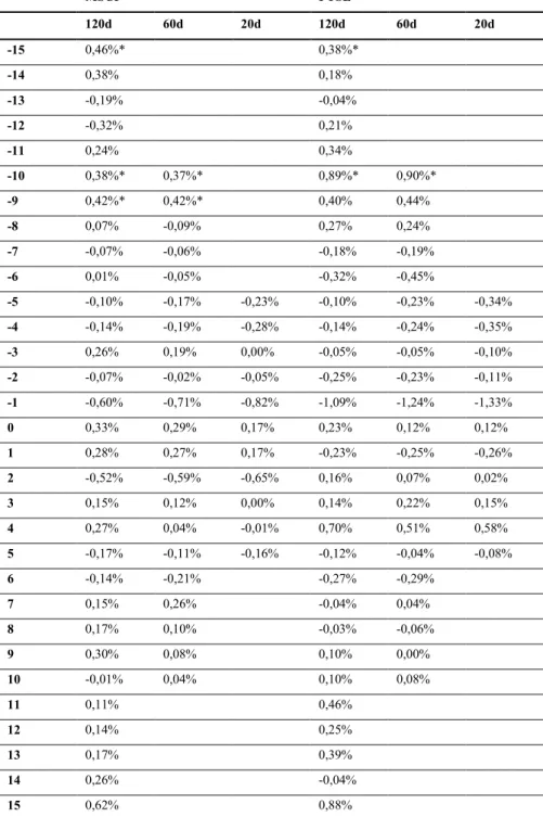
5.1. 120 day Estimation Window

When using the MSCI World index as a market index there is a strange pattern in the trajectory of the cumulative abnormal returns for both the downgraded and the neighbor countries (Figure 3): they appear somewhat constant until day 5 after the downgrade, around 1%, increasing afterwards. Furthermore no single abnormal return is statistically significant at a 95% confidence level, for neither the downgraded nor the neighbor country.

Looking into the case where the FTSE Global was used as the market index (Figure 6), a pattern more in line with previous empirical evidence can be identified: both the downgraded country and the neighbor present a steep upward trajectory which is reversed in the 2 weeks prior to the event, due to persistent negative abnormal returns in that period, but the positive abnormal returns after the event change the trajectory back to the initial path. Nonetheless no single abnormal return was significant, once again, which makes it very difficult to conclude anything regarding the impact of downgrades. One could test if the abnormal returns of the downgraded country and the neighbor countries are different via a t-test, however, different time spans provided (robust) results that answer this question.

5.2. 60 day Estimation Window

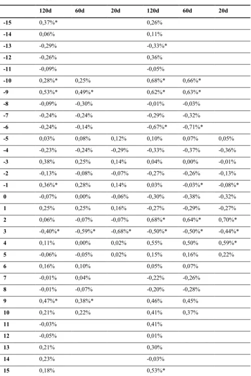
When using a 60 day estimation window better results were obtained, especially in the case of the FTSE (Figure 7). By using the FTSE index there is an obvious downward trend on the cumulative abnormal returns prior to the event, in both downgraded and neighbor countries. As expected the downgraded countries suffer a stronger impact from the downgrade, -1% cumulative abnormal return at the event date, and don’t return to normality after it, as they maintain negative cumulative abnormal returns in 10 days after the event. In the case of the neighbor countries, which present a -0,7% cumulative abnormal return at the event date, the trend is reversed after the downgrade and they return to normality, 0% cumulative abnormal returns, approximately after 10 days. Even though there is no significant abnormal return in the case of the downgraded countries, the neighbor countries present significant abnormal returns in several days, at a 95% confidence level, namely the event date.

The MSCI Index presented, once again, less expected results (Figure 4). Even though there is a milder trend reversion around 5 days after the event, for both downgraded and neighbor countries, it is much milder than in the case of the FTSE Index. Furthermore, the magnitude of the downgrade impact is larger in the national country, which hits its lowest level around -0,5% 6 days after the

event. Moreover only the abnormal return at (t0 + 3) in the neighbor countries is statistically

significant at a 95% confidence level.

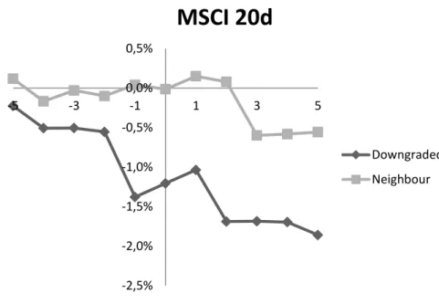
5.3. 20 day Estimation Window

To further reduce any noise that might exist in the estimation window I reduced it to 20 days, approximately one trading month, prior to the beginning of the event window. The event window was also reduced to 5 days, around one trading week, to further increase the accuracy of the significance tests. By doing so I obtained results which are even more aligned with previous empirical evidence, for both the MSCI and the FTSE indexes.

Regarding the FTSE, the negative trend in cumulative abnormal returns is present for both the downgraded and the neighbor countries (Figure 8). For the neighbor countries the lowest point is

attained at (t0 + 1), around -1%, and normality is attained 5 days after the event date (0% CAR).

This group of countries presents several significant negative abnormal returns, at a 95% confidence

trajectory. Their lowest point is attained at (t0 + 1), around -2,5%, but they don’t return to

normality, as the CAR is persistently negative around -2%.

A change in the benchmark index, to the MSCI, changes the trajectory (Figure 5). According to the results attained the negative trend is never reversed. In the case of the neighbor countries the

lowest CAR (-0,6%) occurs at (t0 + 3) and is mildly reversed in the following days. The neighbor

countries on the other hand experience their lowest CAR (-1,9%) at the end of the event window.

However the only significant abnormal return is verified in the neighbor countries at (t0 + 3).

5.4. Remarks

Some remarks must be given regarding the results attained, especially on: the fact that the MSCI performed consistently poorer than the FTSE; the fact that reduced estimation and event windows performed better than longer ones; the fact that in all windows and benchmarks the downgraded countries presented either positive or no abnormal returns at all on the event date.

Looking more carefully into the MSCI World index one can observe it is significantly less diversified than the FTSE Global, which might be affecting the results. As the index has less constituents (6 times fewer constituents than the FTSE), from less countries of origin (half of the countries of the FTSE, and a bigger focus on Europe and the US), the relative weight of the stocks from the countries in the sample might be diluting the abnormal returns. This happens because the market index drops approximately in the same proportion as the country index, instead of keeping itself insulated from the event, enabling to see its impact. In fact 75% of the constituents of the index are companies from the US, UK and Japan, all of them countries represented in the sample both as downgraded countries and neighbor countries. By contrast the truly global reach of the FTSE might act as a barrier between the impact of the national index and the impact on the global index.

According to Mackinlay (1997) there is a trade-off between model accuracy and model stability when considering the length of the estimation window. If on one hand an increased time period can lead to a better model, due to a higher number of observations, the likelihood of encountering noise also increases, decreasing the quality of the model. As the only type of noise controlled for was downgrades in neighbor countries, events like government deficit/superavit announcements

(such as the ones in Brazil due to the corruption scandal Lava Jato) or, more recently, geopolitical actions of high importance (like the Brexit) might be affecting the accuracy of the model, as the national index moves independently from the market portfolio, hence implying a Beta close to 0.

Finally, and perhaps the most striking result, we must analyze why the negative abnormal returns were only found in neighbor countries. By dividing the sample in continents we observe that Europe presents a negative, yet insignificant, abnormal return for the 20 and 60 days estimation windows using both benchmarks (see Table 7); America, both North and South, Asia and Oceania all present positive, however insignificant, abnormal returns for all windows and benchmarks. Having narrowed the question to Europe we can wonder what makes the old continent different from the others. As all data refers to the period after the 2008 financial crisis it overlaps with the European debt crisis. During this period the sustainability of several national debts was questioned, leading some countries to either default, such as Greece, or asking for financial support, like Portugal and Ireland. This support was fundamentally based on austerity measures, hence decreasing national GDP and more importantly for this thesis, Investment, both national and foreign, in the short run. Thus one possible explanation for the abnormal returns verified only in Europe might be the fear of GDP and Investment contraction caused by austerity, which was brought upon by the unsustainable level of national debt, increased by the larger yields implied by lower credit ratings. The uncertain environment during this period, and consequent flight to safety from European investors to non-European stock markets, might have offset the impact of downgrades in these countries, hence canceling possible abnormal returns. One way to assess if this hypothesis is correct is to look into government bond yields for the period analyzed. If there was in fact a flight to safety in the stock market, a parallel one should have occurred in the bond market, as investors typically hold different asset classes in their portfolios. This movement, along with the lower risk premium investors require for holding (what they perceive as) safer assets, would have brought yields down for non-European bonds, while increasing the yields of European bonds. By looking into historical yield to maturities on 10 year government bonds, one can observe that the yield to maturity of Japanese and American bonds decreased constantly from approximately 1,4% and 4% in 2009, to approximately 0,25% and 2,25% in 2015. In Europe some countries did follow this trend (e.g. France and Germany), however, countries like Ireland, Portugal and Spain saw the yields to maturity of their respective bonds increase until early 2013, reaching values well above 10% in the case of Ireland. As such there is some evidence of a flight to safety in the bond market. If a parallel movement occurred in the stock market, it might explain the different reactions to the rating downgrades. Moreover the magnitude of the impacts might have been different for

non-European countries, as countries like the US or Japan were downgraded from AAA to AA+, unlike some of the European countries like Ireland, Portugal or Spain, which were downgraded from Investment grade to Speculative grade. Nonetheless, this flight to safety argument does not explain why neighbor countries feel the impact of the safe economy’s rating downgrade (e.g. Canada suffering a market crash due to USA’s rating downgrade). If there is no impact on the downgraded country, there should be no contagion effect to be spread to neighbor economies.

6. Conclusions

This thesis aimed to explore the impact of downgrades on national stock markets and the spillover effect to neighboring countries. Through an event-study analysis, and consistent with previous theory, I found that downgrades not only influence national stock markets but also leak to their neighbors, with a milder influence.

Regarding the impact at the event date on a national level the analysis suggests that rating downgrades only affect negatively the stock markets in Europe. At a global level there are insignificant positive abnormal returns. As discussed before the safe haven perspective might explain, to some extent, this result. Concerning the spillover effect all models used suggest there are in fact spillover effects at the event date.

Such discoveries should be taken into account in portfolio allocation and can also be the basis of event-driven profit strategies. Regarding portfolio allocation, this thesis highlights how diversification benefits across neighbor countries might be overstated. Such overstatement can be perceived as latent correlation: on regular times the diversification benefits might exist, however, in troubled times, leading to credit downgrades, they diminish significantly, as both markets will react adversely to such event. Concerning event-driven strategies, this thesis suggests that shorting market indexes both in both downgraded and neighbor countries can lead to potential profits. Moreover, going long on sell options, puts, on national and foreign indexes might be an additional method to realize profits.

I found that the choice of benchmark has a big repercussion on the results, especially the power of the tests, and therefore the conclusions one can take. The fact that American, British and Japanese stocks compose around 75% of the MSCI World has a significant impact on the (lack of) results attained in this thesis, a discovery in line with Faias et al. (2012) suggestions.

This thesis is also in line with Makinlay (1997) in respect to both the estimation and the event window length. According to the results there is in fact a trade-off between model accuracy, increasing with bigger estimation windows, and stability, decreasing with bigger estimation windows, due to the noise included, which is very significant at a macroeconomic level. Regarding the event window the results also suggest that shorter windows present more accurate results, which translate in more significant abnormal returns.

Further research could be done on 2 topics. First, one could assess separately the impact of the several types of downgrades. Different impacts for different downgrades, (e.g. AAA to AA vs BBB to BB), would certainly help explain the diverse results attained for Europe. Second, one could investigate the size, as the preliminary evidence of section 5.4 suggests, of the migration of investment funds from Europe to other regions after the outburst of the sovereign debt crisis. If my theory is correct one should verify a significant movement of capital from Europe to these economically developed regions. The fact that there are no abnormal returns on downgrade dates for non-European countries could be reflecting the fact that even though such countries’ credit worthiness was deteriorating, they were seen as a safe haven compared to the rest of the world. Accordingly, the downgrade would have no impact on national stock markets.

Appendix

Table 1: Countries present in the sample

Table 1 presents the countries present in the sample. Countries marked with an asterisk were downgraded during the sample period.

Table 2: Indexes present in the sample

Table 2 presents the indexes selected per country. They follow the order of Table 1 presented above. Indexes marked with an asterisk were downgraded during the sample period.

Table 3: Event dates per country

Table 3 presents the downgrade dates for each country in the sample. They follow the order of Table 1 presented above. Dates marked with an asterisk refer to downgrades done by Moody’s.

Northern Europe Western Europe Southern Europe Great Britain North America South America Eastern Asia Oceania

Denmark Belgium* Italy* Ireland* Canada Argentina* China Australia

Finland* France* Portugal* United Kingdom* Mexico* Brazil* Japan New Zealand*

Norway Germany Spain* USA* Chile South Korea*

Sweden Netherlands* Taiwan

Northern Europe Western Europe Southern Europe Great Britain North America South America Eastern Asia Oceania

OMXC BEL20* FTSEMIB* ISEQ* TSX MERV* SSEC ASX200

OMXH* CAC40* PSI20* FTSE350* IPC* BVSP* JPX NZ50*

OBX DAX IBEX35* SP500* IPSA KS200*

OMX AEX* TWII

Northern Europe Western Europe Southern Europe Great Britain North America South America Eastern Asia Oceania

N/A 16-12-2011 13-07-2012 17-12-2010 N/A 17-06-2014 N/A N/A

10-10-2014* 08-11-2013* 15-03-2011 22-02-2013 14-12-2009* 11-08-2015* 27-01-2011* 29-09-2011*

N/A N/A 13-01-2012* 05-08-2012* N/A N/A

Table 4: Summary statistics for the MSCI World and the FTSE Global returns

Table 4 presents the mean, standard deviation and correlation of returns from the MSCI World index and the FTSE Global index. MSCI World FTSE Global Mean 0,04% 0,04% Standard Deviation 1,00% 0,99% Correlation 41%

Table 5: Average Betas of the MSCI World and the FTSE Global

Table 5 presents the average Betas attained using the Market Model using the MSCI World and the FTSE Global, for the different estimation windows and groups of countries.

Downgraded Neighbor MSCI 20d 0,8800 0,8664 MSCI 60d 0,8776 0,8921 MSCI 120d 0,7861 0,7746 FTSE 20d 0,0909 0,1152 FTSE 60d 0,1616 0,1604 FTSE120d 0,1923 0,1677

Table 6: AAR for downgraded countries from the Event-Study analysis

Table 6 presents the average abnormal returns obtained through the Event-Study analysis of downgraded countries for both market indexes and the several estimation and event windows considered. AARs marked with an asterisk are significant at a 95% level. MSCI FTSE 120d 60d 20d 120d 60d 20d -15 0,46%* 0,38%* -14 0,38% 0,18% -13 -0,19% -0,04% -12 -0,32% 0,21% -11 0,24% 0,34% -10 0,38%* 0,37%* 0,89%* 0,90%* -9 0,42%* 0,42%* 0,40% 0,44% -8 0,07% -0,09% 0,27% 0,24% -7 -0,07% -0,06% -0,18% -0,19% -6 0,01% -0,05% -0,32% -0,45% -5 -0,10% -0,17% -0,23% -0,10% -0,23% -0,34% -4 -0,14% -0,19% -0,28% -0,14% -0,24% -0,35% -3 0,26% 0,19% 0,00% -0,05% -0,05% -0,10% -2 -0,07% -0,02% -0,05% -0,25% -0,23% -0,11% -1 -0,60% -0,71% -0,82% -1,09% -1,24% -1,33% 0 0,33% 0,29% 0,17% 0,23% 0,12% 0,12% 1 0,28% 0,27% 0,17% -0,23% -0,25% -0,26% 2 -0,52% -0,59% -0,65% 0,16% 0,07% 0,02% 3 0,15% 0,12% 0,00% 0,14% 0,22% 0,15% 4 0,27% 0,04% -0,01% 0,70% 0,51% 0,58% 5 -0,17% -0,11% -0,16% -0,12% -0,04% -0,08% 6 -0,14% -0,21% -0,27% -0,29% 7 0,15% 0,26% -0,04% 0,04% 8 0,17% 0,10% -0,03% -0,06% 9 0,30% 0,08% 0,10% 0,00% 10 -0,01% 0,04% 0,10% 0,08% 11 0,11% 0,46% 12 0,14% 0,25% 13 0,17% 0,39% 14 0,26% -0,04% 15 0,62% 0,88%

Table 7: AAR for neighbor countries from the Event-Study analysis

Table 7 presents the average abnormal returns obtained through the Event-Study analysis of neighbor countries for both market indexes and the several estimation and event windows considered. AARs marked with an asterisk are significant at a 95% level. MSCI FTSE 120d 60d 20d 120d 60d 20d -15 0,37%* 0,26% -14 0,06% 0,11% -13 -0,29% -0,33%* -12 -0,26% 0,36% -11 -0,09% -0,05% -10 0,28%* 0,25% 0,68%* 0,66%* -9 0,53%* 0,49%* 0,62%* 0,63%* -8 -0,09% -0,30% -0,01% -0,03% -7 -0,24% -0,24% -0,29% -0,32% -6 -0,24% -0,14% -0,67%* -0,71%* -5 0,03% 0,08% 0,12% 0,10% 0,07% 0,05% -4 -0,23% -0,24% -0,29% -0,33% -0,37% -0,36% -3 0,38% 0,25% 0,14% 0,04% 0,00% -0,01% -2 -0,13% -0,08% -0,07% -0,27% -0,26% -0,13% -1 0,36%* 0,28% 0,14% 0,03% -0,03%* -0,08%* 0 -0,07% 0,00% -0,06% -0,30% -0,38% -0,32% 1 0,25% 0,25% 0,16% -0,27% -0,29% -0,27% 2 0,06% -0,07% -0,07% 0,68%* 0,64%* 0,70%* 3 -0,40%* -0,59%* -0,68%* -0,50%* -0,50%* -0,44%* 4 0,11% 0,00% 0,02% 0,55% 0,50% 0,59%* 5 -0,06% -0,05% 0,02% 0,15% 0,16% 0,22% 6 0,16% 0,10% 0,05% 0,07% 7 -0,01% 0,04% -0,22% -0,26% 8 -0,01% -0,07% -0,20% -0,28% 9 0,47%* 0,38%* 0,46% 0,45% 10 0,21% 0,22% 0,41% 0,37% 11 -0,03% 0,41% 12 -0,05% 0,01% 13 0,21% 0,30% 14 0,23% -0,03% 15 0,18% 0,53%*

Table 8: AAR for downgraded countries in Europe

Table 8 presents the abnormal average returns for European countries alone. Note that at the event date the 60 and 20 days estimation windows columns present negative abnormal returns. AARs marked with an asterisk are significant at a 95% level. MSCI FTSE 120d 60d 20d 120d 60d 20d -15 0,71%* 0,68%* -14 0,32% 0,19% -13 -0,15% -0,18% -12 -0,11% 0,69% -11 0,44% 0,50% -10 0,45% 0,41% 1,22% 1,22% -9 0,68%* 0,68%* 0,71%* 0,77%* -8 0,02% -0,21% 0,41% 0,36% -7 -0,25% -0,23% -0,46% -0,45% -6 -0,59% -0,65% -0,97%* -1,17%* -5 0,05% -0,03% -0,13% 0,12% -0,09% -0,21% -4 0,16% 0,08% -0,08% -0,03% -0,16% -0,24% -3 0,60% 0,49% 0,19% 0,36% 0,36% 0,29% -2 -0,13% -0,04% -0,06% -0,34% -0,30% -0,16% -1 0,30% 0,11% -0,05% -0,11% -0,33% -0,53% 0 0,01% -0,03% -0,21% 0,02% -0,14% -0,20% 1 0,42%* 0,48%* 0,33% 0,18% 0,18% 0,10% 2 -0,14% -0,25% -0,34% 0,47% 0,40% 0,27% 3 -0,51% -0,56%* -0,74%* -0,40% -0,27% -0,27% 4 0,31% -0,10% -0,19% 0,77%* 0,45% 0,50% 5 -0,27% -0,14% -0,22% -0,20% -0,09% -0,09% 6 -0,26% -0,36% -0,47% -0,49% 7 0,07% 0,30% -0,04% 0,10% 8 0,24% 0,19% 0,24% 0,21% 9 0,61% 0,38% 1,07% 0,92% 10 -0,12% -0,01% 0,17% 0,23% 11 0,03% 0,33% 12 -0,08% -0,21% 13 0,48% 0,54% 14 0,17% 0,15% 15 0,41% 1,17%

Figure 1: Ratings of Government Securities for the year of 2012

Figure 1 presents the percentage of Government Securities rated by S&P, Moody´s and other rating agencies in 2012.

Figure 2: Ratings for the year of 2012

Figure 2 presents the percentage of total Securities rated by S&P, Moody´s and other rating agencies in 2012. S&P 47% Moody's 41% Others 12% S&P 45% Moody's 38% Others 17%

Figure 3: CAARs for the MSCI World index using a 120 day Estimation Window

Figure 3 presents the cumulative average abnormal returns obtained using the MSCI index using a 120 day estimation window for both downgraded and neighbor countries.

Figure 4: CAARs for the MSCI World index using a 60 day Estimation Window

Figure 4 presents the cumulative average abnormal returns obtained using the MSCI index using a 60 day estimation window for both downgraded and neighbor countries.

-1,0% -0,5% 0,0% 0,5% 1,0% 1,5% 2,0% 2,5% 3,0% 3,5% -15 -10 -5 0 5 10 15

MSCI 120d

MSCI 60d

Figure 5: CAARs for the MSCI World index using a 20 day Estimation Window

Figure 5 presents the cumulative average abnormal returns obtained using the MSCI index using a 20 day estimation window for both downgraded and neighbor countries.

Figure 6: CAARs for the FTSE Global index using a 120 day Estimation Window

Figure 6 presents the cumulative average abnormal returns obtained using the FTSE index using a 120 day estimation window for both downgraded and neighbor countries.

-2,5% -2,0% -1,5% -1,0% -0,5% 0,0% 0,5% -5 -3 -1 1 3 5

MSCI 20d

FTSE 120d

Figure 7: CAARs for the FTSE Global index using a 60 day Estimation Window

Figure 7 presents the cumulative average abnormal returns obtained using the FTSE index using a 60 day estimation window for both downgraded and neighbor countries.

Figure 8: CAARs for the FTSE Global index using a 20 day Estimation Window

Figure 8 presents the cumulative average abnormal returns obtained using the FTSE index using a 20 day estimation window for both downgraded and neighbor countries.

-1,5% -1,0% -0,5% 0,0% 0,5% 1,0% 1,5% 2,0% -10 -5 0 5 10

FTSE 60d

FTSE 20d

References

Afonso, A. (2003). Understanding the determinants of sovereign debt ratings: Evidence for the two leading agencies. Journal of Economics and Finance, 27(1), 56-74.

Afonso, A., Gomes, P., & Rother, P. (2011). Short‐and long‐run determinants of sovereign debt credit ratings. International Journal of Finance & Economics, 16(1), 1-15.

Afonso, A., Gomes, P., & Taamouti, A. (2014). Sovereign credit ratings, market volatility, and financial gains. Computational Statistics & Data Analysis, 76, 20-33.

Baba, N., McCauley, R. N., & Ramaswamy, S. (2009). US dollar money market funds and non-US banks.

Bangia, A., Diebold, F. X., Kronimus, A., Schagen, C., & Schuermann, T. (2002). Ratings migration and the business cycle, with application to credit portfolio stress testing. Journal of

banking & finance, 26(2), 445-474.

Barron, M. J., Clare, A. D., & Thomas, S. H. (1997). The effect of bond rating changes and new

ratings on UK stock returns. Journal of Business Finance & Accounting, 24(3), 497-509.

Bernanke, B. S., & Blinder, A. S. (1992). The federal funds rate and the channels of monetary transmission. The American Economic Review, 901-921.

Bissoondoyal-Bheenick, E., & Brooks, R. D. (2008). The Impact of Sovereign Ratings Changes: A Comparison of the Market Model, Quadratic Market Model and Downside Model.

Brooks, R., Faff, R. W., Hillier, D., & Hillier, J. (2004). The national market impact of sovereign rating changes. Journal of banking & finance, 28(1), 233-250.

Calvo, S. G., & Reinhart, C. M. (1996). Capital flows to Latin America: is there evidence of contagion effects?.

Cantor, R., & Packer, F. (1994). The credit rating industry. Quarterly Review, 1-26.

Cesaroni, T. (2015). Procyclicality of credit rating systems: how to manage it. Journal of

Economics and Business, 82, 62-83.

Cornell, B., Landsman, W., & Shapiro, A. C. (1989). Cross-sectional regularities in the response of stock prices to bond rating changes. Journal of Accounting, Auditing & Finance, 4(4), 460-479.