1
A Work Project, presented as part of the requirements for the Award of a Masters Degree in Finance from Faculdade de Economia da Universidade Nova de Lisboa
Fearful Asymmetry: An Analysis of Pre-earnings
Abnormal Returns
João Tiago Mira Duarte Amaro
student number 159
A project carried out on the Finance course, with the supervision of:
Pedro Santa-Clara
2 Abstract
In this paper we study the returns on a set of different strategies, which are based on the sign and magnitude of the pre-earnings announcement return for a group of US stocks and for some international markets which provides an additional measure of robustness. We also propose a new methodology for the evaluation of abnormal returns. Evidence is found that stocks with negative abnormal returns on the days prior to the earnings announcement have a subsequent higher return on the days following the announcement. A trading strategy based on these findings is then reproduced and its results are analyzed.
3 1 - Introduction
Can market reaction to earnings be anticipated? The earnings announcement has long been the focus of finance and accounting research. Some study market reaction to unexpected results others focus on trends after the announcement but what if there was a measure known before the event that predicted a trend for the announcement itself?
In this paper we propose a new methodology that aims to do just that by applying the concept of abnormal returns to the period before the earnings announcement and then looking for trends in the subsequent market behavior of stocks. While it seems that in an efficient market such a relation could not exist there are in fact several reasons why this could happen. If there is advanced knowledge of the earnings results by a significant mass of market participants it is possible that this information asymmetry is creating certain distinct patterns which would form before the earnings announcement. It is also possible that due to the increased risk that is present during the earnings period investors perceive their investments differently which would cause them to engage in unusual behaviors.
4
The question we propose to explain is whether these seemingly irrational moves, before the earnings announcements, can give investors a clue to the subsequent market reaction and if this relation is significant to the extent that it can be used to create a trading strategy that can generate meaningful returns to an investor.
2 - Literature Review
The subject of whether the Efficient Market Hypothesis is true and in what form has long been a controversial subject of academic theory with several papers trying to prove its existence while others propose to refute it. Despite this ongoing debate, market anomalies have been documented to exist in the markets.
Such an anomaly is the post-earnings-announcement drift first presented in Ball and Brown (1968). This phenomenon states that a stock with positive (negative) market reaction immediately after earnings announcements tends to have better (worse) performance in the following period. This anomaly has, since then, become the focus of a number of studies.
5
earnings announcements but is very often not accounted for in the estimates released by analysts and find that the EAR methodology is able to generate a better post-earnings drift than the SUE.
It is a fact that most studies related to earnings announcement focus in earnings announcement itself and the post-earnings period. However, in recent years, some papers have started to fill the blank on the pre-earnings research. Of which are an example Affleck-Graves, Jennings and Mendenhall (1994) who focus on the use of insider transactions by institutional investors before earnings announcements and Angel, Christophe and Ferri (2002) who focus on the relation between insider transactions and short-selling during this period. While our objective does not directly involve insider transactions it is in this body of work, market behavior prior to earnings announcements, that this paper is inserted.
3 – Data and Methodology
3.1 – Data
6
workable observations (50.615) due to some missing data and securities that have not been trading since the beginning of the study period.
Additionally, for the purpose of testing whether the findings can be extended to other relevant international markets we collected the same information for the constituents of the FTSE 100, DAX, CAC 40 and Nikkei 225.
Daily returns of the indices studied were also collected as a proxy for market returns in that country as well as 3-month US treasury bills for risk-free returns. All returns and earnings dates were taken from Bloomberg. Treasury bills were obtained from the US treasury website.
3.2 - Methodology
In this paper we introduce a new methodology to look for abnormal returns (in excess of the market) in the days prior to the announcement date. For that purpose we use two different methods of estimating pre-earnings market reaction.
The Average Abnormal Return (AAR) is a measure of the average behavior of stock on the days preceding the earnings announcement. This will be calculated as the return of the stock minus the average return of the market in those n days.
= , − , (1)
7
The use of the market return allows for a better assessment of relative performance of the security when compared to the market as a whole on each day. This enables the abnormal return to work as a form of comparison between stocks by measuring divergence from the mean.
The Successive Abnormal Return (SAR) is a measure of the average behavior of stock on the days preceding the earnings announcement. This works similarly to a dummy variable that indicates whether the company had positive (1) or negative (-1) abnormal returns in all of the n days (and their signal). In case it presented mixed abnormal returns SAR will be defined as 0.
= 1 , − , > 0, ∀ ∈ 1, (2)
= −1 , − , < 0, ∀ ∈ 1, (3)
Where , is the return of stock at time , , is the market return at time , is the earnings announcement date and is the number of observed days before the event.
8
For a sub-group of the S&P 500 sample (8792 observations) the data contains the actual time during the day when the announcement took place which allowed for a more narrow post-event period of a single trading day which is the return from the close on to + 1 in case the release is made after market close or the close on − 1 to when it is made either before market open or during trading hours.
Due to the complexity of integrating data from two different sources into a single database and the huge amount of observations, matlab and a computer script developed using the python programming language were used in addition to a conventional spreadsheet application. This significantly reduced the computational power and time needed to develop the calculations and at the same time enabled more complex procedures that would not have been possible otherwise.
4 - Results
4.1 – Average Abnormal Return
For the AAR method we analyze different values for the number of observed days in order to establish which measure can give an investor better returns. The values chosen are 3, 5, 10 and 20.
9
quite weak when compared to any negative AAR measure even the ones with lower results. If we reflect on the fact that the holding period for each trade is merely two days we can see that the expected return of the negative AAR over a year is quite large (even accounting for the fact that earnings announcements are generally condensed in a small time period during each quarter).
The strategy presents the best results for S&P Mid (1,27% 3 day AAR) and worst for S&P 500 (0,91%), but the difference between these samples is not very significant which seems to indicate that this effect is independent of company size.
The economic significance of the results demands that we further analyze with more attention the returns on a strategy based on a 3 day negative Average Abnormal Return which have a great return profile and at the same time make for a more parsimonious model that involves fewer inputs than the longer AAR measures.
To further study the 3 day AAR measure we estimated the following regression:
= # + $ ∗ (4)
Where R is the compounded return of a stock for the event, AAR is the corresponding 3 day AAR measured before the event and alpha and beta are estimated regression parameters.
10
intercepts which seem to indicate that holding stocks through the earnings announcement period is generally slightly profitable. We can also see from the t-tests that all estimated parameters are significantly different from 0 at a 95% confidence level (p-values are all 0%). R-squared, as expected in a predictive regression, is quite low at 1% for the three size based samples.
It is also interesting to observe the behavior of expected returns for more demanding negative values of AAR. In Table 3 we can see that for the S&P 500 lower values of AAR will have a higher expected return where 0 has the lowest return (0,91%) and –PI% the best (4,21%), however being more demanding also means that there will be less investment opportunities. Over the course of the sample (11 years) there were only 243 observations, for the S&P 500, where AAR was lower than –PI% (compared with 8636 for lower than 0), this translates into about 22 per year. Standard deviation also tends to become higher for lower AAR (16,7%) which signifies that even though the returns are better they are more volatile. These values appear to be quite robust as the p-values are 0% for the hypothesis that returns are equal to 0.
11
The S&P SMALL index is the sample which presents more investment opportunities through the period. This is especially true for the more demanding values of AAR where the quantity of observation with AAR lower than –PI% (476) is much larger than for the other two samples (243 for S&P 500 and 196 for S&P MID) to such a degree that it cannot be simply explained by the greater number of components in this index (600 compared to 500 and 400). This leads us to believe that a smaller company is more likely to present extreme values of AAR which could be related to the fact that generally small stocks are more volatile than larger stocks. This is also reflected in the standard deviation which is greater than what was observed in the other two samples (9,4% for negative AAR compared with 7,1% and 7,7%). As before p-values are all 0%.
An analysis of Figure 1 shows that the assumption that stock returns follow a normal distribution is not verified for stocks with negative AAR. We can see that there is a positive skewness (right tail is longer) and that the distribution has a higher peak (kurtosis is 18,71) than the normal distribution. The negation of this assumption has implications for the use of standard deviation as an effective measure of risk.
4.2 – Successive Abnormal Return
For the SAR method we compute statistics only for the 3 day SAR case. The reason for this is that this test requires that abnormal returns have the same sign every day, so
1
12
increasingly higher values will be more restrictive and generate samples that are too small to be analyzed with the degree of robustness we desire for this study.
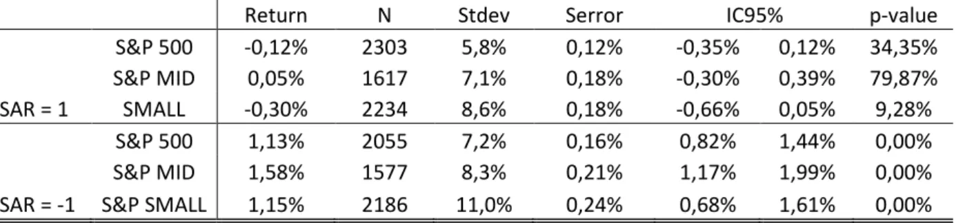
In Table 4 we can see that the SAR method, like the AAR method, finds low returns for stocks that had positive abnormal returns in the days prior to the earnings announcements (-0,12% for S&P 500). From the analysis of the confidence intervals and p-values, at a 95% confidence interval, statistically we cannot exclude the hypothesis that the average return is in fact equal to zero.
On the other hand, stocks with negative SAR present high expected returns (1,13% for S&P 500) and as before the mid-sized stocks appear to be the best investment choice (1,58%). Volatility also displays the pattern seen before where smaller stocks present higher volatility in the time around the earnings. Once again p-values are all 0%.
We have shown that a strategy based on the SAR method can also be used to generate high returns. However since the two strategies are not independent (a stock with negative SAR will necessarily also have negative AAR) combining the two strategies should not improve the results.
4.3 – Timed Data
13
This sub-sample, while smaller, presents descriptive statistics very similar to what was observed before in the full sample which leads us to believe that partitioning the sample has not introduced any sort of bias that could put into question if our findings would work similarly for the full S&P 500.
From these results we can construct strategies that invest every day in the stocks that will be presenting results in the following day. Because the number of required investments differs from day to day, sometimes consisting of a single security, we define various levels of maximum portfolio exposure to a single stock in the portfolio.
Table 5 shows that, as expected from the average returns per trade, the strategy is much more profitable (115%) than the S&P 500 index which for this period had a negative average return (-0,83%). From an absolute return perspective using a negative AAR strategy with no investment limit yields the best results but this is also the riskiest strategy as it means that sometimes the whole portfolio is invested in a single security. What is most curious is that some of the more limited strategies (25% and 10% limits) have a standard deviation similar to that of the S&P 500 (21,3% standard deviation) which could imply similar risk but with much better returns. To compare the various strategies we chose the Sharpe ratio as a risk adjusted measure of performance and find that results are very similar for all different limits, although the limited strategies seem to have a slight advantage (2,30 compared with 2,16 for the no-limit strategy).
14
in this study, should be a concern for an implementation of this strategy. The fast rotation of the portfolio and short window of opportunity for buying the stocks also makes this strategy quite difficult to implement in a large scale.
4.4 - International Markets
Another important question that needs to be asked is whether this phenomenon is restricted to the US or is it present in other markets. To test this we use samples from the main international markets in developed countries. The chosen markets were United Kingdom, France, Germany and Japan. For each of these markets stocks were chosen from the main index for each market which should contain the largest and most representative stocks from that country. These indices are respectively: FTSE 100, CAC 40, DAX and Nikkei 225.
These markets were chosen because of the fact that data is available, for earnings and returns, in long time series as well as the fact that this markets are largely considered to be the most liquid after the US which should reduce the risk of market imperfections distorting the results.
15
sample. For Japan the sample size should not be an issue (6029 observations), however this is a market notorious for behaving differently than the rest which may imply this phenomenon is related to a behavior characteristic of western investors not present in Japan.
5 - Random Days
From the analysis made in the previous chapters we can determine that these strategies which exploit abnormal returns in the days previous to the earnings announcements can generate large returns. However, it is essential to establish if this is solely true for the days studied or if it is a phenomenon that is present every day. A possibility is that the strategy is only describing a short-term mean reversal that is not exclusive to earnings dates. The short-term mean reversal is a known effect that following large changes in price stocks will suffer a reversal in the opposite direction.
For this purpose we randomly pick 18000 dates from the time period used in the above samples and match this to the constituents of the S&P 500. We then compute descriptive statistics in order to establish if there is a significant difference between this sample and the S&P sample from before.
16
in regular days, even after large relative declines, stocks will be, in the following days, less volatile than around earnings.
However, it is curious to see that the frequency of stocks that pass the AAR criteria is not that different in the two samples. From that one may conclude that even though stocks are more volatile after the earnings announcement they present the same trading patterns before earnings announcements as they do on regular days. Due to the very low standard errors of the random sample (0,04%), even though average returns are not very large (0,21%) they are still significantly different from zero at a 95% confidence level for negative values of AAR.
A Q-Q plot of the two samples (Figure 2) was used to further compare the two samples. It corroborates the evidence found, by showing that they have a linear trend in the quartiles’ relationship, but this trend has a low slope which means that the observed values at each quartile are generally greater for the Earnings sample, as predicted from the analysis of the mean differences. The values deviate most from this trend in the lower left side of the figure which implies that during earnings days, a company presenting bad results is expected to have its stock lose more than in the worse days of regular trading.
17 6 – Potential Causes
After we have consistently established the robustness of this relationship it is important to discuss some of the possible reasons that may be behind this phenomenon. We are interested in knowing why certain stocks are heavily sold by investors in the days prior to the earnings announcements, while others are accumulated. There must be a fundamental reason behind this behavior which if known could further propel the development of more efficient and specialized abnormal return measures for the pre-earnings period.
The initial assumption that such a relation could be present because of the effect of insider trading is dispelled as the evidence shows a reversal in pre-earnings trends which means there is a higher sale pressure on these stocks before the announcement which would not be expected from investors that have gained access to information regarding the announcement before the market.
Another possible reason is that we are seeing stocks that have, in the past earnings seasons, disappointed investors which are now afraid to hold this stocks during the earnings period because of fear that the situation will repeat itself. Investor fear of the earnings announcement has been a discussed topic in the field of behavioral finance.
To empirical test the probability of a stock having negative AAR dependant on it having disappointed in the past we used the following probit regression:
18
Where the dependent variable is defined as 1 if the stock has a negative AAR and 0 otherwise, D is a dummy variable that states whether the stock disappointed (measured as a negative return during the earnings period) in the last earnings announcement and alpha and beta are estimated parameters.
The parameters were obtained using the maximum likelihood estimation method. We find that # is equal to 46,47% and the $ parameter which is associated with the variable D is 1,95%. This means that the probability of having negative AAR is 1,95% higher for stocks that presented disappointing results in the last quarter. While past disappointments seem to explain part of the phenomenon a significant relation cannot be established between these and negative AAR to fully explain the effect.
Anticipated regret, as discussed by Zeelenberg (1999) poses that individuals make their decisions influenced by the possibility they will later come to regret it and tend to avoid such situations. This may explain why some stocks have a significant reduction in price prior to the earnings announcement. Investors fearing they may later come to regret holding the stock during the earnings period decide to sell it before the announcement.
19 7- Conclusions
We have in this paper shown that it is possible to use AAR and SAR to identify stocks that have a higher expected return for the earnings announcement period. We find an asymmetric behavior for stocks with negative and positive abnormal returns. We have also shown that the implementation of these results can produce strategies that look very favorably when compared with a traditional buy and hold investment strategy, both in terms of average returns and risk adjusted measures.
The results found are both statistically significant and economically significant. An investor following this strategy in the last 10 years could have had an average return of 115% per year compared to -0,83% for an investment in the S&P 500 which is a fantastic result even when adjusted for the additional risk.
We concluded that by isolating stocks with negative AAR or SAR we can identify better returns and that by using more demanding variations of these strategies can produce better average returns but at the expense of less investment opportunities. We show that this phenomenon is not exclusive to the US companies of the S&P 500, S&P Mid and S&P Small but is also present in other developed markets.
20
Finally we presented some possible theories that try to explain the reasons for the occurrence of these opportunities. While we rejected the initial working hypothesis of insider trading as the cause of this phenomenon we find some evidence for the presence of investors fear based on previous disappointments.
References
Aboody, David, Reuven Lehavy and Brett Trueman. 2008. “Limited Attention and the Earnings Announcement Returns of Past Stock Market Winners”.
Affleck-Graves, John Felix, Robert H. Jennings and Richard R.Mendenhall. 2005. “Evidence of Informed Trading Prior to Earnings Announcements”, Working Paper. Angel, James J., Michael G. Ferri, and Stephen E. Christophe. 2004. "Short Selling Prior to Earnings Announcements", Journal of Finance, 59(4): 1845-1875.
Ball, Ray and Philip Brown. 1968. “An Empirical Evaluation of Accounting Income Numbers”, Journal of Accounting Research, 6: 159-178.
Bauman W. S, C.M. Conover and R.E. Miller. 1998. “Growth versus Value and Large-Cap versus Small-Cap Stocks in International Markets”, Financial Analysts Journal, May/April: 75-89.
21
Bernhardt, D. and D. Campello. 2007. “The dynamics of earnings forecast management”, Review of Finance 11: 287–324.
Bollerslev, Tim, Julia Litvinova and George Tauchen. 2006. “Leverage and Volatility Feedback Effects in High-Frequency Data”, Journal of Financial Econometrics, 4(3): 353-384.
Brandt, M. W., R. Kishore, P. Santa-Clara, and M. Venkatachalam. 2006. “Earnings announcements are full of surprises”, Working Paper.
Campbell, John Y., Andrew W. Lo and A. Craig MacKinlay. 1997. The Econometrics of Financial Markets. Princeton, NJ: Princeton University Press. Princeton.
Wong, M. 1997. “Abnormal Stock Returns Following Large One-day Advances and Declines: Evidence from Asia-Pacific Markets”, Financial Engineering and the Japanese Markets, 4(2): 171-177.
22
Table 1. Average return divided in positive and negative AAR for the three S&P size based samples. AAR is calculated for the ranges going from the earnings day to 3, 5, 10 and 20 days before. The return values presented are average holding period returns per observation of each sample.
AAR(3) AAR(5) AAR(10) AAR(20) S&P 500
<0 0,91% 0,92% 0,84% 0,79% >0 0,22% 0,21% 0,28% 0,32% S&P MID
<0 1,27% 1,26% 1,11% 1,06% >0 0,29% 0,33% 0,46% 0,51%
S&P SMALL
<0 1,04% 1,07% 0,95% 0,85% >0 0,07% 0,06% 0,13% 0,20%
Table 2. Regression results for the three S&P samples estimated using the OLS method. T is the t-statistic value for the parameter besides it. IC95% is the lower and upper bound of a 95% confidence interval. R2 is the r-square value.
Coefficient T IC95% p-value R2
Α 0,58% 11,45 0,48% 0,67% 0,00%
0,01 S&P 500 β -0,36 -9,81 -0,43 -0,28 0,00%
Α 0,80% 12,34 0,67% 0,92% 0,00%
S&P Mid Β -0,40 -9,10 -0,49 -0,32 0,00% 0,01
Α 0,59% 8,93 0,46% 0,72% 0,00%
23
Table 3. Descriptive statistics for different levels of negative AAR for the three S&P samples. Return is the average holding period return per event, N is the number of events that pass the AAR condition, Stdev and Serror are respectively standard deviation and standard error and IC95% is the lower and upper bound of a 95% confidence interval.
Return N Stdev Serror IC95% p-value
<-PI% 4,21% 243 16,7% 1,07% 2,11% 6,31% 0,01%
<-2% 2,27% 797 12,4% 0,44% 1,41% 3,13% 0,00% <-1% 1,64% 2559 9,2% 0,18% 1,29% 2,00% 0,00% S&P 500 <0 0,91% 8636 7,1% 0,08% 0,76% 1,06% 0,00% <-PI% 4,75% 196 13,5% 0,96% 2,87% 6,64% 0,00% <-2% 2,83% 616 12,1% 0,49% 1,88% 3,78% 0,00% <-1% 2,14% 2063 9,6% 0,21% 1,72% 2,55% 0,00% S&P MID <0 1,27% 6487 7,7% 0,10% 1,09% 1,46% 0,00%
<-PI% 3,85% 476 19,0% 0,87% 2,15% 5,55% 0,00%
<-2% 2,63% 1324 14,6% 0,40% 1,84% 3,41% 0,00% <-1% 1,66% 3496 11,5% 0,19% 1,28% 2,05% 0,00% S&P SMALL <0 1,04% 9095 9,4% 0,10% 0,84% 1,23% 0,00%
Table 4. Descriptive statistics for different levels of SAR for the three S&P samples.
Return N Stdev Serror IC95% p-value
S&P 500 -0,12% 2303 5,8% 0,12% -0,35% 0,12% 34,35% S&P MID 0,05% 1617 7,1% 0,18% -0,30% 0,39% 79,87% SAR = 1 SMALL -0,30% 2234 8,6% 0,18% -0,66% 0,05% 9,28%
S&P 500 1,13% 2055 7,2% 0,16% 0,82% 1,44% 0,00%
24
Table 5. Comparison of statistics for a buy and hold strategy on the S&P 500 and negative AAR strategies involving different levels of maximum portfolio exposure. Return is the average return per year, Stdev the annualized standard deviation and Sharpe the sharpe ratio calculated with a 3,23% risk-free interest rate according to the
formula = ) )+ *.
SP500 Negative AAR
No limit 50% 25% 10%
Return -0,83% 115,48% 87,04% 59,83% 33,23% Stdev 21,3% 51,9% 36,4% 24,8% 13,1%
Sharpe -0,19 2,16 2,30 2,29 2,29
Table 6. Descriptive statistics of returns for stocks presenting negative AAR in the UK, France, Germany and Japan.
Return N Stdev Serror IC95% p-value
FTSE 100 0,92% 895 6,4% 0,21% 0,50% 1,34% 0,00%
CAC 40 0,55% 361 5,4% 0,29% -0,01% 1,11% 5,45%
DAX 0,70% 486 5,3% 0,24% 0,23% 1,17% 0,39%
Nikkei 225 0,40% 6029 5,2% 0,07% 0,26% 0,53% 0,00%
Table 7. Descriptive statistics of returns for stocks presenting negative AAR in days independent of earnings announcements. Difference is the difference between the return of the Earnings sample and the Random sample. Confidence intervals for the difference are calculated using a two-sample unpooled t-test.
Return N Stdev Serror IC95% p-value
Random 0,21% 8137 4,0% 0,04% 0,12% 0,30% 0,00%
Earnings 0,91% 8636 7,1% 0,08% 0,76% 1,06% 0,00%
25
Figure 1. Histogram with frequency of returns for S&P 500 stocks with negative AAR. Superimposed is a normal distribution with the same mean and standard deviation.