Technology adoption deterrence through learning and capacity investment

WORKING PAPER SERIES

CEEAplA WP No. 05/2007

Technology Adoption Deterrence through

Learning and Capacity Investment

Ricardo Cabral

Technology Adoption Deterrence through

Learning and Capacity Investment

Ricardo Cabral

Universidade da Madeira (DGE)

e CEEAplA

Working Paper n.º 05/2007

Maio de 2007

CEEAplA Working Paper n.º 05/2007 Maio de 2007

RESUMO/ABSTRACT

Technology Adoption Deterrence through Learning and Capacity Investment

This paper analyzes an incumbent’s use of learning and manufacturing capacity investment to deter or accommodate adoption of a new technology by a potential competitor, using a perfect state-space equilibrium concept and a model motivated by the semiconductor industry. The results indicate that, under typical market conditions, an incumbent leaves some capacity idle after learning-by-doing cost reductions have been achieved, and an incumbent that follows an accommodation strategy invests in more learning than a monopoly that does not face the threat of entry. Finally, the analysis suggests that investments in learning and manufacturing capacity allow early adopters to credibly alter strategies (and equilibria) of the adoption game in their favor vis-à-vis followers.

KEYWORDS: Technology adoption, deterrence, learning-by-doing. JEL classification: L11, L13, L6

Ricardo Cabral

Departamento de Gestão e Economia Universidade da Madeira

Edifício da Penteada Caminho da Penteada 9000 - 390 Funchal

Technology adoption deterrence through learning and

capacity investment

Ricardo Cabral* [email protected] Universidade da Madeira Departamento de Gestão e Economia

Campus da Penteada 9000-390 Funchal

Portugal

December 15th, 2006

Abstract

This paper analyzes an incumbent’s use of learning and manufacturing capacity investment to deter or accommodate adoption of a new technology by a potential competitor, using a perfect state-space equilibrium concept and a model motivated by the semiconductor industry. The results indicate that, under typical market conditions, an incumbent leaves some capacity idle after learning-by-doing cost reductions have been achieved, and an incumbent that follows an accommodation strategy invests in more learning than a monopoly that does not face the threat of entry. Finally, the analysis suggests that investments in learning and manufacturing capacity allow early adopters to credibly alter strategies (and equilibria) of the adoption game in their favor vis-à-vis followers.

JEL classification: L11, L13, L6

Keywords: Technology adoption, deterrence, learning-by-doing

*

The paper is based on a chapter of my doctoral dissertation. I gratefully acknowledge financial support from PRAXIS XXI, FCT, Portugal. I appreciate comments by Henry Chappell and John McDermott. The views

1. Introduction

The semiconductor industry, and for that matter the LCD (liquid-crystal-display) flat

screen industry, which shares semiconductor technology, has experienced a relentless pace of

technological change over the last decades. For example, capital outlays per semiconductor

plant increased 10 times between the 1980s and the mid-1990s to 1 billion USD while the

lifetime of a plant fell to 5 years (Hall and Ziedonis, 2001) and the number of transistors that

could be manufactured in a chip die area grew exponentially. Still the semiconductor industry

is highly cyclical and often unprofitable. The LCD flat screen industry evolution has been even

more impressive, with the first worldwide 7th generation plant (from LG Philips), which

entered in production in January 2006, costing 5.7 billion USD. Yet LG Philips has recently

experienced large losses as prices for LCD TVs fell rapidly, and has cut its capital investment

plans by two thirds. Other firms in the LCD industry face similar pressures, and the supply glut

is expected to increase with the launch of two additional new generation plants by Sharp and

AU.1

These industries are characterized by steep learning curves that result in substantial

reductions in marginal cost with growing cumulative output (Flamm, 1993; Dick, 1994; Cabral

and Leiblein, 2001; Siebert, 2002). For example, the ESIA (2005) estimates a 30% average cost

decline with each doubling of cumulative output. Furthermore, investment in plant capacity is

typically lumpy, with long lead times to build and bring the plant to commercial operation.

Perhaps as a consequence of these characteristics, the race to adopt the next technology

through investment in manufacturing capacity remains a feature of the industry, with firms

seeking to adopt the next process technology and to explore learning externalities as rapidly as

possible. However, given the low industry profitability over the years, one wonders why firms

This paper puts forward the hypothesis that the apparently “excessive” investments in

capacity follow from the characteristics of the industry, namely the importance of

learning-by-doing and the existence of lumpy capacity investments. Therefore, we seek to analyze whether

and in what manner an incumbent uses learning and capacity investments as strategic variables

in a technology adoption game, using a perfect state-space equilibrium model (Fundenberg and

Tirole, 1986). In the model a larger manufacturing capacity enables larger output levels and

thus faster learning. Learning derived from production experience results in decreasing

marginal production costs, a feature typical of many industries.

The results show that the incumbent, under typical market conditions, leaves some

capacity idle in the second stage, once it has managed to reduce its marginal costs through

learning by doing, even if it does not face the threat of competitive entry. Furthermore, an

incumbent that accommodates adoption of the technology by a competitor invests in more

learning and in more capacity than a monopoly that does not face the threat of entry under

comparable market conditions. In summary, the results of the analysis suggest that the

investments in learning and manufacturing capacity are strategic in that they permit an early

adopter to position itself more advantageously in the market (i.e., have lower marginal costs,

higher output, and higher profitability) vis-à-vis followers. By means of this investment in

learning and capacity the incumbent may be able to alter its costs sufficiently so as to be able

to adopt a credible deterrence strategy and in equilibrium deter entry. Moreover, even if the

incumbent follows an accommodation strategy, through investment in learning and capacity

the incumbent is able to change the competition game to its advantage.

This paper is organized as follows: Section 2 provides the background to the choice of

the equilibrium concept used in this analysis (perfect state-space equilibria). Section 3

2. Background

Most strategic behavior adoption models (Reinganum, 1981a; Quirmbach, 1986)

consider only “precommitment” or “open-loop” equilibria, where firms precommit to the

adoption dates and to output levels at the beginning of the game. Each firm is assumed to

maintain their initial (precommitted) strategies regardless of the game history. Thus, the

“precommitment equilibria are really static, in that there is only one decision point for each

firm,” (Fudenberg and Tirole, 1986, p.8). By contrast, closed-loop strategies (Fundenberg and

Tirole, 1986; Kamien and Schwartz, 1991; Gilbert and Harris, 1984) are time and state

dependent, meaning that the optimal firm strategy at each point in time depends not only on

time, but also on the level of one or more state variables, which are dependent on present and

past decisions (e.g., capital stock, experience). The closed-loop equilibria are Nash equilibria

in the closed-loop strategies (Fudenberg and Tirole, 1986).

Past analyses of strategic interaction with learning have for the most part been based on

open-loop models where firms simultaneously commit themselves to entire time-paths of the

control variable, e.g. output rates (Spence, 1981; Baldwin and Krugman, 1988; Helpman and

Krugman, 1989). Note that given the firm’s optimal closed-loop strategy, it is possible to

define a precommitment strategy which replicates the closed loop strategy at each point in

time. The difference is that the precommitment strategy depends only on time, and that if the

state variable were to vary off its “precommitted” path, or the firm’s rivals behaved

irrationally, the precommitment strategy no longer would be an equilibrium, whereas the

closed-loop strategy would, because the firm’s closed-loop strategy is contigent on the rival’s

actions. The closed-loop strategy specifies the firm’s strategy for all possible contigencies of

the state variables, whereas the open-loop strategies only result in equilibria along the

Given that learning-by-doing is an obvious example of a state-dependent variable, a

perfect state-space equilibrium imposes a stronger consistency requirement on closed-loop

equilibria by requiring that for every possible initial state, the closed-loop strategies form a

closed-loop equilibrium (Fudenberg and Tirole, 1986).2 The goal of this paper is to develop a

model to identify the perfect state-space (closed-loop) equilibria in time of adoption, capacity,

and capacity utilization rate for a two-stage duopoly game with potential adoption in the

second period.

3. Model

The model proposed here follows Fudenberg and Tirole (1985, 1986), Dasgupta and

Stiglitz (1988), and Tirole (1988), but introduces additional decision factors: time of adoption,

capacity and utilization rate rather than just output. That is, the output rate is not forced to be

100% in both stages (full capacity utilization), thus providing one additional degree of

freedom, and changing the game from a precommitment game (“open-loop”) to a state

dependent closed-loop game. Earlier research has not focused on the impact of

learning-by-doing on capacity investments and their joint impact on technology adoption, but has instead

analyzed different important issues related to capacity investment. Gabszewicz and Poddar

(1997) show that under Cournot competition and uncertain demand there will be investment in

excess capacity. Besanko and Doraszelski (2004) argue that a lower degree of irreversibility in

the investment in capacity leads to more aggressive competition. Pacheco-de-Almeida and

Zemsky (2003) on the hand argue that the existence of a time lag between the investment

decision and production, leads to a firm preference towards incremental capacity investments.

The strategic interaction between the firms is modeled using a two-stage duopoly game

potential competitor deciding whether to adopt the process technology in the second stage. The

adoption of a new process technology is realized by means of an investment in manufacturing

capacity (a new plant). The new process technology allows the manufacture of new or

differentiated (higher quality) products.3 The incumbent (firm A), makes a capacity investment

decision in the first stage and also chooses the output level for the first stage. In making those

choices, the incumbent has two possible endogenous strategies: deter adoption or

accommodate adoption in the second stage. In the second stage, the potential competitor (firm

B) decides whether to adopt the process technology and at what capacity level. Firm A

observes whether firm B adopts the process technology or not, by observing the capacity

investment by firm B. If firm B does adopt, the two firms then play a Cournot game. If firm B

does not adopt, firm A remains a monopoly in the second stage and makes its output decision

accordingly.

3.1. Model specification

The reduction in marginal costs from learning is modeled, following Dasgupta and

Stiglitz (1988) and Tirole (1988), as:

0 , ₂ 1 0 2 = − ⋅ A A > A c c q c c

where qA1 is firm’s A output in the first period, cA2 is the incumbent’s marginal cost in the

second period, c is the incumbent’s marginal cost in the first period, and c0 is the

learning-by-doing cost coefficient. Learning-by-learning-by-doing is firm-specific and reduces the incumbent’s

marginal costs between the two stages but not within stages. Output, qin, is equal to the

capacity utilization rate, uin, times the capacity, Ki.

B B B A A A A A A u K q u K q u K q ₁= ₁⋅ , ₂ = ₂⋅ , ₂ = ₂⋅

where the 1, 2 and A, B are the period and the firm indices, respectively. Initial investment

costs decrease linearly over time and are specified by:

F T( _0i,K_i)=α₀ −α₁⋅T_0i +α₂⋅K_i (1)

The discount factor between each period is δ<1. Output produced in a given period

must be sold in that period, i.e., output cannot be stored between stages. Finally, the market is

characterized by linear demand behavior in each stage:

p a q p a q q A A B 1 1 1 2 2 2 = − = − −

where again 1, 2 and A, B are the period and the firm indices, respectively. The market

expands between stage 1 and stage 2 (a2>>a1), and each firm’s output is the product of the

utilization rate and the firm’s capacity.

In this analysis only pure strategy Nash equilibria are considered, and quantity (not

price) is the relevant decision variable, which can be justified by the relatively lengthy

production cycles in semiconductor fabrication. The game is solved by backward induction for

an incumbent that follows an accommodation strategy, for an incumbent (monopoly) that does

not face the threat of entry, and finally for an incumbent that follows an adoption deterrence

strategy.

3.2. Accommodation strategy

In a two-stage game framework firm A’s objective function is given by:

π_A =π_A1+ ⋅δ π_A2 = p q₁⋅ _A1− ⋅c q_A1−F T( ₀ =0,K_A)+ ⋅δ π_A2 (2)

Firm A has three possible capacity utilization choices which are endogenously

determined in the model: (i) produce at full capacity in the first stage (‘ramp-up’ production),

stages; (iii) produce at less than full capacity in the first stage (build-up idle capacity), and at

full capacity in the second stage.4

Firm B will adopt the new process technology if its profit maximization problem has a

positive solution: max ( , ) . . , , U K B B B B B B B B B p q c q F T K s t u K 2 2 2 2 0 2 2 1 0 1 0 0 π π = ⋅ − ⋅ − = ≤ ≤ ≥ ≥ (3) where qB2 =uB2 ⋅KB.

With accommodation, firm B adopts the technology in the second stage and the two

firms then play a Cournot game. Then, the non-negativity utilization rate and capacity

constraints are not binding (uB2 ,KB >0), and given firm’s A output in the second stage firm B’s

problem is solved by maximizing:

L (uB2,Kb, )λ =(a2 −qA2 −qB2 −c q)⋅ B2 −(α0 −α1+α2⋅KB)+λ(1−uB2) (4)

The Kuhn-Tucker conditions with respect to the first choice variable (utilization rate)

are: u u and u B B B 2 2 2 0 1 0 ⋅ ∂ = − = ∂ λ L ( )

which, after some simplifications, result in

u_B u_B q_B a qA c 2 2 2 2 2 0 1 2 = ∨ = ∨ = − − (5)

The Kuhn-Tucker conditions with respect to the second choice variable (capacity) are

equivalent to: K K B B ⋅ ∂ = ∂ L 0,

which can be rewritten as (a2 −qA2 − ⋅2 qB2 −c u)⋅ B2 =α2 (6) KB qB a q c A =0 ∨ = − − − 2 2 2 2 α2 (7)

and both (5) and (7) must be simultaneously satisfied at the optimum. From (5) and (7) it

follows that there is a corner solution5, i.e., one of the constraints is binding. Since firm B

enters in the second stage, then KB , uB2>0, and it can be shown that:

u_B2 1 q_B2 K_B a2 qA2 c 2

2

= ∧ = = − − −α (8)

that is, if firm B does enter in the second stage, it produces at full capacity. It is now necessary

to check that the second-order sufficient conditions for constrained maximization are satisfied.

Rewriting firm B’s Lagrangean function (4) as:

L

B( , , )u K λ =π( , )u K +λ⋅g u K( , )

where the indices are omitted from uB2, and KB to simplify the notation, and g(u,K)=1-u is the

capacity utilization constraint. It then follows that:

π ∂ π ∂ uu B u K K = = − ⋅ < ∀ ≠ 2 2 2 2 0, 0, (9) π ∂ π ∂ KK B K u u = = − ⋅ < ∀ ≠ 2 2 2 2 0, 0, (10) ∂ ∂ ∂ ∂ g u g g K g u K = = −1, = =0 (11) and since π and g are twice continuously differentiable functions:

∂ π ∂ ∂ ∂ π ∂ ∂ 2 2 2 2 4 2 B B A B u K = K u =a −q − − ⋅c q (12)

The second order sufficient condition for a constrained maximum is that the

π π π π uu uK u Ku KK K u K g g g g 0 0 >

and substituting in the values computed above in equations (9) through (12), we obtain

π π π π π uu uk Ku KK KK u − − = − = ⋅ > 1 0 1 0 0 2 2 0

which is true, since u*B2 =1. Thus, equation (8) is the solution to firm B’s profit maximization

problem.6 Firm B’s profit is then given by:

π_{B =}h − ⋅α −qA α α   2 2 2_ − − 2 0 1 2 2 ( )

where h2=a2-c+α2 . Since the two firms are playing a Cournot game, Firm A’s problem in the

second stage is:

max . . U A A A A A A A p q c q s t u 2 2 2 2 2 2 2 2 0 1 0 π π = ⋅ − ⋅ ≤ ≤ ≥

and its Lagrangean is

L (uA2, )λ =(a2 −qA2 −qB2)⋅qA2 −(c c− 0⋅qA1)⋅qA2 +λ(1−uA2) (13) resulting in:

(

)

where again h2=a2-c+α2 , and qB2 is given by (8). Since this is a one-variable constrained

maximization problem the second order sufficient condition is:

∂ ∂ ∂π ∂ L A A A A A u u K 2 2 2 2 2 2 0 = = − ⋅ < (15)

and since KA is strictly positive by assumption, equation (15) is always satisfied, i.e. firm A’s

profit function is a strictly concave function on the capacity utilization rate, and therefore equation (14) is the solution to the profit maximization problem.

Firm A’s profit in the second stage then is:

π_A h c qA 2 2 0 1 2 2 9 = ( + ⋅ ⋅ ) (16)

Thus, in the first stage firm A (the incumbent) maximizes:

L_{(uA ,KA, ) (a qA c q) A ( KA)} (h c qA ) _{( u )} A 1 1 1 1 0 2 2 0 1 2 1 2 9 1 λ = − − − α +α ⋅ +δ + ⋅ ⋅ +λ − (17)

and solving this maximization problem yields:

u q K a c h c c h h c c A1 A1 A 1 2 4 9 2 0 8 9 0 2 1 4 9 2 0 8 9 0 2 1 2 2 = ∧ = = − − + ⋅ ⋅ ⋅ − ⋅ ⋅ = + ⋅ ⋅ ⋅ − ⋅ ⋅ α δ δ δ δ (18)

where h1=a1-c-α2 . Now, substituting (18) into (14) results in

u u q q h c h h c h A A A A 2 2 2 1 2 0 1 1 4 3 0 2 1 2 2 3 1 = ∨ = = ⋅ + ⋅ ⋅ ⋅ + ⋅ ⋅δ ⋅ < (19) Therefore, if h h c c a c a c c c 2 1 0 0 2 0 1 2 0 2 3 2 6 4 6 4 3 6 4 2 6 4 < ⋅ ⋅ − ⋅ − ⋅ ⋅ ⇔ < ⋅ − ⋅ − − ⋅ − ⋅ ⋅ + − ( ) ( ) ( )( ) ( ) δ α δ α (20)

firm A will choose to produce at less than full capacity utilization rate in the second stage (uA2<1), with: u h c h h c h q h c h c A2 A 2 0 1 1 4 3 0 2 2 2 0 1 4 3 0 2 2 2 3 1 3 = ⋅ + ⋅ ⋅ ⋅ + ⋅ ⋅ ⋅ < ∧ = + ⋅ − ⋅ ⋅ δ δ (21)

and total profits for firm A will be:

π δ δ δ α A h h h c h c = + ⋅ ⋅ ⋅ ⋅ + ⋅ ⋅ ⋅ − ⋅ ⋅ − 1 2 8 9 1 2 0 4 9 2 2 4 9 0 2 0 4 1( ) (22) where

π δ δ δ δ α A h c h c h h c h c 1 1 8 9 0 2 1 4 9 0 2 1 4 9 0 2 4 9 0 2 2 0 4 1 = − ⋅ ⋅ ⋅ − ⋅ ⋅ ⋅ + ⋅ ⋅ ⋅ ⋅ − ⋅ ⋅ − ( )( ) ( ) (23) π δ A c h h c 2 0 1 2 2 4 9 0 2 2 9 1 = ⋅ + ⋅ − ⋅ ⋅ ( ) ( ) (24)

are the first- and second-period contributions, respectively for the profit function, as defined in (2). Because the capacity utilization constraint is binding in the first stage7, the second order sufficient condition for the unconstrained maximization problem is:

(

)

since both KA and uA1 are strictly positive, and δ and c0 are both less than 1. Firm A’s profit

function is strictly concave and the solution (22) is a maximum. Expressions (23) and (24) show that while the second-period profit is always non-negative, as expected, the first-period profit contribution (excluding the fixed cost, α0) may be negative, i.e., variable costs may be

larger than total revenues. The first-period profit may be negative if the second-period demand is sufficiently larger than the first-period demand, i.e., if the market is growing rapidly, or if learning is very important (c0 is large) and the future is not heavily discounted (δ≈1). This

result indicates that under the conditions described above, the incumbent sacrifices first-period profits, i.e., sets price below marginal cost in the first stage and overproduces so as to move down the learning curve.

On the other hand, if (20) is not satisfied, i.e., if

2 2 3 1 3 2 6 4 6 4 2 0 1 1 4 3 0 2 2 1 0 0 ⋅ + ⋅ ⋅ ⋅ + ⋅ ⋅ ⋅ > ⇔ > ⋅ − ⋅ − ⋅ ⋅ h c h h c h h h c c δ δ ( ) ( )

then market demand in the second period is much larger than in the first period and the optimal capacity utilization rate of the incumbent in the second stage is uA2=1. Thus, the incumbent’s

first stage is then reduced to choosing the capacity KA, and first period utilization rate, uA1,

which maximizes the discounted present value of profits:

π_A =π_A1+ ⋅δ π_A2 = p q₁⋅ _A1− ⋅c q_A1−F T( ₀ =0,K_A)+ ⋅δ (p₂⋅K_A−c_A2⋅K_A)

The Lagrangean in this case is:

L

and it then follows that:

u u K h h c A1 A1 A 1 12 2 0 0 1 2 2 = ∨ = ∧ = + ⋅ ⋅ + − ⋅ ⋅       ∨ δ δ δ u h c h c h c h c K h c h c c A1 A 1 0 2 2 0 2 0 1 2 0 2 0 1 2 0 0 2 2 2 1 2 2 2 2 2 = ⋅ ⋅ + ⋅ ⋅ + ⋅ − ⋅ ⋅ + ⋅ − ⋅ ⋅ − ⋅ ∧ = ⋅ + ⋅ − ⋅ − ⋅ ⋅ − ⋅       δ δ α δ α δ δ α δ δ δ ( ( )) ( ) ( ) ( ) ( ) ( ) (25) If h h c c 2 1 0 0 3 2 6 4 6 4 > ⋅ − ⋅ − ⋅ ⋅ ∧ ( ) ( δ ) δ δ α δ α δ ⋅ ⋅ + ⋅ ⋅ + ⋅ − ⋅ + ⋅ − ⋅ ⋅ − ⋅ > ( ( )) ( ) ( ) 2 2 1 2 2 2 1 1 0 2 2 0 2 0 1 2 0 h c h c

h c h c , then uA1=1 and the

incumbent produces at full capacity in both stages. Otherwise,

u h c h c h c h c A1 1 0 2 2 0 2 0 1 2 0 2 2 1 2 2 2 1 = ⋅ ⋅ + ⋅ ⋅ + ⋅ − ⋅ ⋅ + ⋅ − ⋅ ⋅ − ⋅ < δ δ α δ α δ ( ( )) ( ) ( ) q h c h c c A1 1 1 2 0 2 2 0 0 1 2 = + ⋅ ⋅ ⋅ + ⋅ − − ⋅ δ α δ ( ) ( )

and the incumbent produces at less than full capacity in the first stage and at full capacity in the second stage, that is, if demand in the second stage is sufficiently large, the incumbent builds more capacity than it needs in the first stage, which it uses only in the second stage. Thus, demand growth and learning both contribute to an increase in the optimal capacity investment. However, while learning creates the incentive to leave the capacity idle in the second stage as technology matures, demand growth on the other hand creates the incentive to leave capacity idle in the first stage.

Table 1 and 2 about here

The optimal accommodation strategy depends on market characteristics. In particular, the constraints specified in Table 2 define the optimal path of the capacity utilization rate in the two stages. The second-period output and the total profits corresponding to each of these strategies are given in the next tables. These accommodation strategies are based on the assumption that in fact firm B adopts the technology (the conditions under which firm B adopts the technology will be explored later).

For this to be a subgame perfect equilibrium, the conjectures have to be consistent. In this case, firm B’s profits have to be positive, and firm A cannot be better off by pursuing an adoption deterrence strategy.

Table 3 and 4 about here

Since the alternative strategies result in different output levels in the second stage, it is clear that firm B’s output and profit will depend on which strategy is being followed. The accommodation strategy requires that firm B enter the market in the second stage, and this means that firm B must have positive profits if it enters in the second stage.

π_{B =}h − ⋅α −qA α α      − − > 2 2 2 2 0 1 2 2 ( ) 0

For the case where uA2<1 (firm A produces at less than full capacity in the second stage) this reduces to:

π δ δ α α α B c h c h c = − ⋅ ⋅ ⋅ − ⋅ ⋅ ⋅ − ⋅ ⋅ −       − − ( ) ( ) ( ) 6 4 3 2 9 4 0 2 2 0 1 0 2 2 2 0 1

The results indicate that firm B’s profitability of adoption in the second-stage increases with market growth, with the discount rate (lower discount factor δ), and with the reduction in the fixed costs over time, α1, but decreases with the first period market size, with the

learning-3.3. Two-stage monopoly model with no threat of competitive adoption

The optimal incumbent (monopoly) strategy when there is not the threat of adoption by a competitor, for example, due to regulatory barriers, is again determined from the generic profit maximization problem (2). In this case, however, the firm is also a monopoly in the second stage. The analysis is similar to the accommodation case and the results are the following: u K h c a c c u a c c K K u a c c K K K c a c a c c u A A A A A A A A A A 1 1 12 0 2 1 2 0 2 2 2 0 1 12 0 1 2 0 1 2 2 1 2 0 2 2 1 2 2 2 2 1 = ∧ = + ⋅ ⋅ − − ⋅ ∧ = − + ⋅ ⋅         ∨ = − + ⋅ ⋅ ⋅ ∧ = ⋅ ⋅ − + ⋅ − − ⋅ − ⋅ ∧ =         δ δ δ δ δ α δ δ ( ) ( ) ( ) ( ) (26)

The optimal first-stage output and total profits for a monopoly are presented in Table 5, where it should be noted that qA1=KA , h2 -α2=a2 -c, and the results refer to a case where the

optimal monopoly strategy is to produce at full capacity in the first period and at less than full capacity in the second period. Interestingly, depending on the parameters of the model, the optimal first period accommodation output can be larger or smaller than the optimal monopoly output (with no threat of adoption).8

Table 5 about here

The intuition is that for a given level of output in the second stage, a reduction in the marginal costs in the second stage increases accommodation profits more than it increases monopoly profits. Under accommodation, the reduction in firm A’s marginal cost contributes to an increase in firm A’s output directly (through the first order condition marginal revenue=marginal cost) and indirectly by shifting the firm A’s residual demand curve to the right (firm B decreases its output in response to firm A’s decrease in cost). Consequently, it is

possible that under certain conditions, the monopoly will invest less in learning (produce less in the first period) than an incumbent which will face adoption in the second stage. This suggests that, under certain conditions, competition leads to a higher investment in learning as argued by Cabral and Riordan (1994).

If the optimal monopoly strategy results in a second period output choice which is larger than the adoption deterrence output, then the incumbent is a “natural” monopoly. In this case, the capacity and the utilization rates are given by equation (26). However, in most cases, firm A is not a natural monopoly and its optimal strategy will be either an accommodation strategy or a deterrence strategy. In the latter case, the monopoly sacrifices some of its profits to deter adoption (relative to the case where there is no threat of adoption) but, depending on the parameters of the model, will achieve deterrence profits above the accommodation profits.

3.4. Adoption deterrence strategy

To deter adoption, firm A has to build enough capacity and produce enough output in the first stage to credibly make adoption in the second stage unprofitable for any potential competitor. That is, if firm B adopts, the incumbent’s optimal accommodation output in the second stage will be such that the entrant (firm B) will not have positive profits:

π_{B =}h − ⋅α −qA acc α α      − − < 2 2 2 2 0 1 2 2 0 ( ) ( ) , (27)

It was shown above that profits of firm B are negative when firm A’s output is larger than the deterrence output. So, for the adoption deterrence strategy to be credible if B adopts, then (27) is equivalent to

q_A2(acc)>q*_A2(det)=h₂− ⋅2 α₂− ⋅2 α₀−α₁ (28)

qA acc KA qA acc h c q K A A 2 2 2 2 0 1 3 ( )= ∨ ( )= + ⋅ ⋅ < (29)

Therefore, if firm A intends to pursue an adoption deterrence strategy, its general profit maximization problem becomes:

max , ( ) ( , ) . . , , (det) , (det), * * π π δ π δ π π α α α A A A A A A A A A A A A A A A A u K a q q c q F T K s t u h c q q h K q 1 1 2 1 1 1 1 0 2 1 2 0 1 2 2 2 0 1 2 0 0 1 0 2 3 2 2 = + ⋅ = − ⋅ − ⋅ − = + ⋅ ≤ ≤ ≥ + ⋅ ⋅ > = − ⋅ − ⋅ − >

where q*A2 (det) is the adoption deterrence output in the second stage.

In the first stage, the incumbent chooses the utilization rate and capacity so that, if adoption occurs, its optimal output response given by (29) would still be sufficient to deter adoption. In the second stage, adoption will in fact be deterred and the incumbent will be a monopoly which maximizes:

max ( ) . . π π A A A A A A A A u a q q c q s t u 2 2 2 2 2 2 2 2 2 0 1 0 = − ⋅ − ⋅ ≤ ≤ ≥

The deterrence analysis developed in the rest of this section considers only one of the strategic cases described earlier. Specifically, it is assumed that the optimal accommodation strategy is to produce at full capacity in the first stage and at less than full capacity in the second stage. In this case, the capacity utilization constraint is not binding in the second stage

(uA2<1) and firm A’s optimal output in the second stage if adoption occurs, is given by:

qA h c q A 2 2 2 0 1 3 = + ⋅ ⋅ (30)

For credible adoption deterrence, if adoption does occur in the second stage then the optimal output given by (30) must also satisfy (28). Since in this scenario the second-period

optimal output is only a function of model parameters and the first period output, this condition then is equivalent to a constraint on the first-period output

q q h c A1 A1 2 2 0 1 0 3 3 > ∗ = − ⋅ − ⋅ − (det) α α α (31)

where q*A1(det) is firm A’s first stage output level which makes firm B indifferent between

adopting or not adopting the process technology (threshold adoption deterrence output). Firm B observes firm A’s first period output and is able to determine whether adoption will be profitable or not, by comparing it with the adoption deterrence level, q*A1(det). Therefore, to

deter adoption firm A’s problem then becomes: max , ( ) ( , ) . . , (det) π π δ π δ π α α α π A A A A A A A A A A A A A A u K a q q c q F T K s t u q q h c 1 1 2 1 1 1 1 0 2 1 1 1 2 2 0 1 0 0 0 1 3 3 0 = + ⋅ = − ⋅ − ⋅ − = + ⋅ ≤ ≤ > = − ⋅ − ⋅ − ≥ ∗

where qAi =uAi ⋅KA and πA2 is the solution to the problem:

max ( ) . . π π A A A A A A A A u a q q c q s t u 2 2 2 2 2 2 2 2 2 0 1 0 = − ⋅ − ⋅ ≤ ≤ ≥

In the second stage, firm A first observes whether firm B adopts or not (invests in a new fab), and then chooses the output level. Thus, firm B estimates its profitability of adoption from the outcome of a Cournot duopoly game (NE), although if adoption is in fact deterred, firm A will produce monopoly output in the second stage, rather than the Cournot duopoly output. The solution for these two problems is:

(

)

If qA1>q*A1(det), the deterrence constraint is not binding, and the optimal deterrence output is feasible: q q h h c c c c A1 A1 2 1 0 2 0 2 0 1 0 2 0 2 2 4 3 3 4 4 2 > ⇔ < ⋅ ⋅ + ⋅ ⋅ − ⋅ + ⋅ − ⋅ − ⋅ − ⋅ ⋅ * α ( δ ) α α ( δ ) δ (32)

The deterrence strategy can thus be solved for analytically, and its profitability for the different scenarios compared with the optimal accommodation strategy. The firm will choose the most profitable of these two strategies.

The notation used in the analysis is the following: q*A1(det) is the threshold deterrence

output, which is the minimum output level in the first stage required to deter firm B from entering in the second stage; qA1(acc) is the optimal, profit-maximizing, adoption

accommodation output in the first stage, assuming that adoption does occur in the second stage; qA1(mon) is the profit-maximizing first period monopoly output, assuming that there will

be no adoption in the second stage (i.e. firm A is a monopoly in both stages because adoption is prohibited). Thus, for any adoption deterrence equilibria, output must be greater or equal than the threshold deterrence output, q*A1(det). Likewise, for any accommodation strategy,

output levels above q*A1(det) will also not be equilibria.

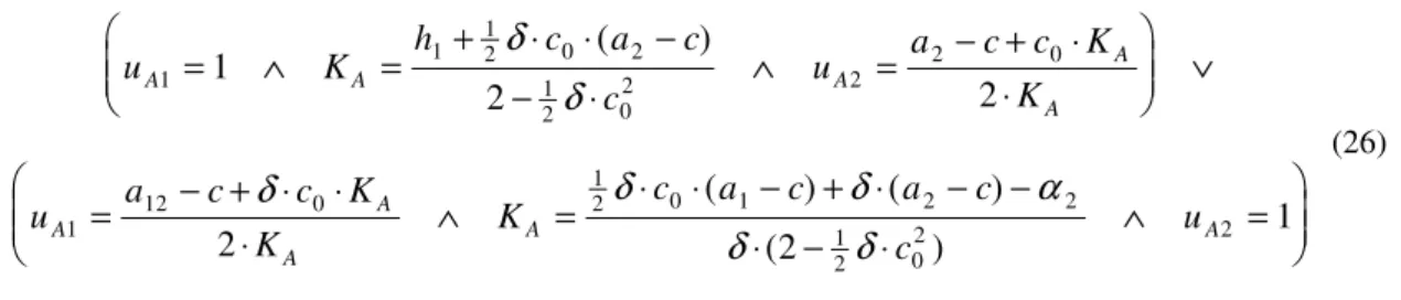
Therefore, accommodation and monopoly strategies will be simultaneously feasible if and only if qA1(acc)<q*A1(det)<qA1(mon), and it then follows that π(qA1(acc))<π(qA1(mon)). In

this reasoning, it is assumed that the deterrence threshold constraint is not binding (see Figure 1(a)). The feasible (i.e. consistent) deterrence and accommodation output levels are plotted in bold, whereas the non-feasible (off equilibrium space) output levels are represented with a dashed line.

When the deterrence constraint is binding the problem’s complexity is increased and the analysis is the following: First, assume that the optimal accommodation output is smaller than the monopoly output (q (acc)<q (mon)). Then, deterrence will be preferred unless the

deterrence threshold is so high that a boundary solution is achieved where the profitability of deterrence is lower than the profitability of accommodation (see Figure 1(b)).

Figure 1 about here

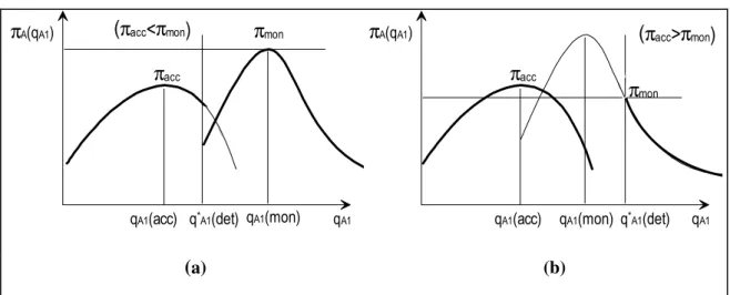
Next, assume that the optimal accommodation output is larger than the optimal monopoly output, qA1(acc)>qA1(mon). qA1(mon) will be a perfect state-space equilibrium if

q*A1(det)<qA1(mon), in which case the optimal first period monopoly output does deter

adoption and beliefs are consistent (see Figure 2(a)). If q*A1(det)>qA1(mon), the choice between

a deterrence or accommodation strategy is not clear. In fact, when

qA1(mon)<q*A1(det)<qA1(acc), or even when qA1(acc)<q*A1(det) but q*A1(det) is sufficiently

close to the accommodation output, deterrence may be preferred if the monopoly profits in the second stage are large enough to compensate for the profit loss derived from the deviation from the optimal first stage accommodation output: (see Figure 2(c) and (e)).

Figure 2 about here

In Figure 2, the profitability of the deterrence strategy (πmon) and the profitability of the accommodation strategy (πacc) are plotted as functions of first stage output (and capacity) choice by the incumbent, firm A. Again, the feasible (i.e. consistent) deterrence and accommodation output levels are plotted in bold, whereas the non-feasible (off equilibrium space) output levels are represented with a dashed line. For example, an accommodation strategy above the deterrence threshold is not feasible and is represented by a dashed line. Similarly, a monopoly strategy below the deterrence threshold is not feasible and is also represented with a dashed line.

The game has a subgame perfect equilibrium. In the second stage of this equilibrium, if firm B enters, both firms will play a Cournot duopoly game, but if firm B does not enter, firm

A will choose monopoly output, regardless of its first period strategy choice.

In Figure 2(a) optimal deterrence is feasible, and firm A will pursue a deterrence strategy. Note that since the accommodation output qA1(acc) is larger than the threshold

deterrence output, q*A1(det), the accommodation output would in fact deter adoption in the

second stage, and thus firm A’s beliefs would not be consistent and the accommodation strategy would not be a Nash equilibrium. In Figure 2(b) and (d) firm A will always accommodate, since it is always more profitable to do so. This is the situation one will find when the market is growing too rapidly, and the adoption deterrence output is very large. Figure 2(c) and (e) represent boundary solutions, where the adoption deterrence threshold output, q*A1(det), constrains the maximum profitability of the adoption deterrence strategy, but

where the deterrence strategy is still the optimal strategy. Finally, it is conceivable that

q*A1(det) could be such that the payoffs from the deterrence and accommodation strategies

would be the same, and thus the incumbent would be indifferent between the two strategies. Thus, the parameters of the model will determine whether deterrence is always preferred (πmon>πacc), accommodation is always preferred (πmon<πacc), or whether the incumbent is indifferent between the two strategies (πmon=πacc).

4. Conclusion

This paper developed a two-stage adoption model with capacity constraints and learning-by-doing, and sought to determine the perfect state-space (closed-loop) strategies in an incumbent and follower game. It was shown that, depending on exogenous characteristics such as learning rate or market growth, the incumbent may prefer either to accommodate or to

deter adoption. The incumbents’ optimal strategy under typical market conditions is to leave a part of its manufacturing capacity idle in one of the stages, depending on whether the learning effect or the demand growth effect dominates, i.e., the incumbent invests in “excess” capacity. Moreover, the results suggest that under typical conditions an incumbent following an accommodation strategy invests in more learning and in more “excess” capacity than a comparable monopoly that does not face the threat of adoption by a competitor. That is, competition or the threat of competition leads to more investment in learning and capacity.

Finally, the results are consistent with setting price below static marginal cost during the initial stages of production when demand growth is large, and with declining prices over time.

5. References

BALDWIN, R. AND KRUGMAN, P. “Market Access and International Competition: A Simulation Study of 16K Random Access Memories.“ in Robert E. Feenstra (editor), Empirical Methods for International Trade, Cambridge, Massachusetts: MIT Press, 1998, pp. 171-202.

BESANKO,D. AND DORASZELSKI,U. “Capacity Dynamics and Endogenous Asymmetries in Firm Size.“ RAND Journal of Economics, v.35 (2004), pp. 21-49.

CABRAL,L. AND RIORDAN,M.“The learning curve, market dominance, and predatory pricing.“ Econometrica, v.62 (1994), pp.1115-1140.

CABRAL,R. AND LEIBLEIN,M. “Adoption of a Process Innovation with Learning-by-Doing: Evidence from the Semiconductor Industry.“ Journal of Industrial Economics, v. 49 (2001), pp. 269-280.

DASGUPTA,P. AND STIGLITZ,J. “Learning By Doing, Market Structure and Industrial and Trade Policies.“ Oxford Economic Papers, v. 40 (1988), pp. 246-68.

DICK,A. “Accounting for semiconductor industry dynamics”, International Journal of Industrial Organization, v. 12(1994), pp. 35-51.

ESIA(EUROPEAN SEMICONDUCTOR INDUSTRY ASSOCIATION),“2005COMPETITIVENESS REPORT”,2005.

FLAMM,K. “Semiconductor Dependency and Strategic Trade Policy.“ Brookings Papers on Economic Activity: Microeconomics, No. 1 (1993), pp. 249-333.

FUDENBERG,D. AND TIROLE, J. “Learning by doing and market performance”, Bell Journal of Economics, v. 14(1983), pp. 522-530.

__________________________ “Preemption and Rent Equalization in the Adoption of New Technology”, Review of Economic Studies, v. 52 (1985), pp. 383-401.

__________________________ Dynamic Models of Oligopoly, Chur, Switzerland: Harwood Academic Publishers, 1986.

GABSZEWICZ, J. AND PODDAR, S. “Demand Fluctuations and Capacity Utilization under Duopoly”, Economic Theory, v. 10(1997), pp. 131-147.

GILBERT,R. AND HARRIS,R. “Competition with lumpy investment.“ RAND Journal of Economics, v. 15(1984), p. 197-212.

HALL, B. AND ZIEDONIS, R. “The patent paradox revisited: an empirical study of patenting in the U.S. semiconductor industry, 1979-1995”, RAND Journal of Economics, v. 32(2001), pp. 101-128.

HELPMAN,E. AND KRUGMAN,P. Trade Policy and Market Structure, Cambridge, Massachusetts: The MIT Press, 1989.

KAMIEN,M., AND SCHWARTZ, N.Dynamic Optimization, 2nd Edition, Amsterdam: North-Holland Publishers, 1991.

PACHECO-DE-ALMEIDA, G., AND ZEMSKY, P. “The effect of time-to-build on strategic investment under uncertainty.” RAND Journal of Economics, v.34 (2003), pp. 167–183.

QUIRMBACH, H. “The diffusion of new technology and the market for an innovation”, Rand Journal of Economics, v. 17(1986), pp. 33-47.

REINGANUM, J. “On the Diffusion of New Technology: A Game Theoretic Approach”, Review of Economic Studies, v. 48(1981), pp. 395-405.

SIEBERT, R. “Learning by Doing and Multiproduction Effects over the Life Cycle: Evidence from the Semiconductor Industry“ Discussion Paper FS IV 02-23, Wissenschaftszentrum Berlin, 2002.

SPENCE,M. “The Learning Curve and Competition”, Bell Journal of Economics, v. 12(1981), pp. 49-70. TIROLE,J.The Theory of Industrial Organization, Cambridge, Massachusetts: The MIT Press, 1988.

Appendix 1. Figures

qA1(acc) q*A1(det) qA1

πA(qA1) πacc (πacc<πmon) qA1(mon) πmon qA1 πA(qA1) qA1(acc) πacc

qA1(mon) q*A1(det)

(πacc>πmon)

πmon

(a) (b)

qA1(acc)

qA1(mon) qA1

q*A1(det)

πA(qA1)

πacc

πmon (πacc<πmon)

q*A1(det) qA1(acc)

qA1(mon) qA1 πA(qA1) πmon (πacc>πmon) πacc (a) (b) qA1(acc)

qA1(mon) q*A1(det) qA1

πA(qA1)

πmon

(πacc<πmon)

πacc

qA1(acc)

qA1(mon) q*A1(det) qA1

πA(qA1) πacc πmon (πacc>πmon) (c) (d) qA1(acc) qA1(mon) qA1 πA(qA1) πacc πmon (πacc<πmon) q*A1(det) (e)

Figure 2: Deterrence vs accommodation when accommodation output is larger than the optimal monopoly output

Appendix 2. Tables

Exogenous Parameters Definitions

a1 demand in first period

a2 demand in second period

δ discount factor c static marginal cost c0 learning coefficient

α₀ fixed plant cost

α₁ decline over time in fixed cost α2 marginal cost of capacity

h1 h1=a1-c-α2 h2 h2=a2-c+α2

Endogenous Variables Definitions

qA1 (mon) first period monopoly output

qA2 (mon) second period monopoly output

qA1 (acc) first period accommodation output

qA2 (acc) second period accommodation output

qA1*(det) first period deterrence output threshold

qA2*(det) second period deterrence output threshold

uA1 firm A’s first period utilization rate

uA2 firm A’s second period utilization rate

uB2 firm B’s second period utilization rate

KA firm A’s capacity choice

KB firm B’s capacity choice

πA (mon) firm A’s profits under monopoly

π_A (acc) firm A’s profits under accommodation strategy πA1 (mon) firm A’s first period profits under monopoly

π_A1 (acc) firm A’s first period profits under accommodation π_B firm B’s profits

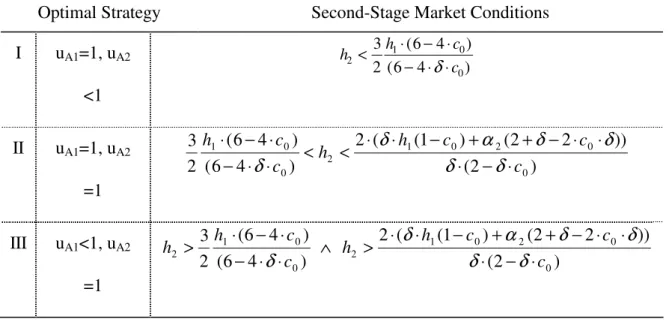
Optimal Strategy Second-Stage Market Conditions I uA1=1, uA2 <1 h h c c 2 1 0 0 3 2 6 4 6 4 < ⋅ − ⋅ − ⋅ ⋅ ( ) ( δ ) II uA1=1, uA2 =1 3 2 6 4 6 4 2 1 2 2 2 1 0 0 2 1 0 2 0 0 h c c h h c c c ⋅ − ⋅ − ⋅ ⋅ < < ⋅ ⋅ − + + − ⋅ ⋅ ⋅ − ⋅ ( ) ( ) ( ( ) ( )) ( ) δ δ α δ δ δ δ III uA1<1, uA2 =1 h h c c 2 1 0 0 3 2 6 4 6 4 > ⋅ − ⋅ − ⋅ ⋅ ∧ ( ) ( δ ) h h c c c 2 1 0 2 0 0 2 1 2 2 2 > ⋅ ⋅ − + + − ⋅ ⋅ ⋅ − ⋅ ( ( ) ( )) ( ) δ α δ δ δ δ

Table 2. Accommodation strategies in capacity utilization rate

Optimal Strategy Second Stage Output

I uA1=1, uA2 <1 q h c h c A2 2 0 1 4 3 0 2 3 = + ⋅ − ⋅ ⋅δ II uA1=1, uA2 =1 _q h h c A2 1 12 2 0 2 2 = + ⋅ ⋅ + − ⋅ ⋅ δ δ δ III uA1<1, uA2 =1 q h c h c c A2 2 0 1 2 0 0 2 2 2 = ⋅ + ⋅ ⋅ − ⋅ − ⋅ ⋅ − ⋅ δ δ α δ δ δ ( ) ( )

Table 3. Optimal second stage output of the incumbent

Optimal Strategy Profits

I uA1=1, uA2 <1 _π δ δ δ α A h h h c h c = + ⋅ ⋅ ⋅ ⋅ + ⋅ ⋅ ⋅ − ⋅ ⋅ − 1 2 8 9 1 2 0 4 9 2 2 4 9 0 2 0 4 1( ) II uA1=1, uA2 =1 π δ δ δ δ α A h h h h h c = − ⋅ + ⋅ ⋅ + ⋅ ⋅ + ⋅ ⋅ + − ⋅ ⋅ − 4 8 4 8 2 2 1 2 1 2 2 2 2 2 2 0 0 ( )

III uA1<1, uA2 =1 π_{A A} α _A α _A δ A A α

A h q q K h K c K K = − + ⋅ − ⋅ + ⋅ − + ⋅ ⋅      ⋅ − ( _{1 1 2}) _{1 2} 2 2 0 ₀ 2

Accommodation Monopoly q h h c c A1 1 4 9 2 0 8 9 0 2 2 = + ⋅ ⋅ ⋅ − ⋅ ⋅ δ δ q h c h c A1 1 1 2 0 2 2 1 2 0 2 2 = + ⋅ ⋅ ⋅ − − ⋅ ⋅ δ α δ ( ) π δ δ δ α A h h h c h c = + ⋅ ⋅ ⋅ + ⋅ − ⋅ ⋅ − 1 2 8 9 1 2 0 4 9 2 2 16 9 0 2 0 4 ( ) π δ α δ α δ α A h h h c h c = + ⋅ ⋅ − + − − ⋅ − 1 2 1 2 2 0 2 2 2 0 2 0 4 ( ) ( ) ( )

Table 5. Output and profitability of accommodation and monopoly strategies

1 _{Financial Times, Nov. 30, 2006 “LG Philips scales back screen dream”.}

2 _{For example: In a two-stage game with an incumbent and a potential entrant in the second stage, assume the best strategy is}

to deter adoption. Adoption deterrence is achieved by increasing output in the second stage to a level which makes adoption unprofitable. A precommitment deterrence strategy would be to commit in the first period to a second period output which deters adoption. A perfect precommitment equilibrium requires that if adoption occurs, the incumbent maintain its original production target, and that this be its best possible choice for both possible scenarios (adoption and no adoption). This equilibrium is clearly not credible in this context, as after adoption the incumbent would adjust its response to an accommodative strategy. In a perfect (state-space) closed-loop equilibrium, the firm’s second period output could be contingent on adoption and some state variable (experience), and the incumbent could choose a strategy which would penalize adoption and yet be its optimal choice if adoption does occur, but not penalize the incumbent in the second-stage if adoption does not occur.

3 _{For example, again according to the FT (see Footnote 1) a 7}th

generation LCD manufacturing plant allows the production of 42- and 47- inches flat screen TVs, whereas a 8th generation LCD plant would allow the manufacture of 50-inches flat screen TVs.

4

This would occur if the market size in the second stage is so much larger (and profitable) to justify building more capacity than you need for the first stage. A strategy with less than full capacity utilization in both stages is not consistent with profit maximization since capacity is costly.

5 _{Substituting (5) into (7) we get 0⋅}

uB2 =α2 . But this cannot be true since capacity is costly (α2>0), and firm B adopts the

technology in the second stage (KB>0).

6

If the capacity utilization constraint were not binding the results would differ substantially. In fact, the second order sufficient conditions for a maximum would then be:

π π π π π π π π π uu KK uu uK Ku KK uu KK uK K u = − ⋅ < = − ⋅ < = ⋅ − > 2 0 2 0 0 2 2 2

and after some calculus this can be shown to be equivalent to: α < ⋅2 (a − −c q )

7 _{Since, by assumption the capacity utilization constraint is not binding in the second stage, then it must be binding in the first}

stage. Otherwise, the incumbent could increase profits by adopting at a smaller scale.

8

However, the first period accommodation output of a Stackelberg quantity game where the incumbent is the leader, qA1

(acc,Stackelberg), is always larger than the first period monopoly output:

q acc Stackelberg h c h c A1 1 1 2 0 2 0 2 2 ( , ) = + ⋅ ⋅ ⋅ − ⋅ δ δ π δ δ δ α A acc Stackelberg h c h h h c ( , ) = + ⋅ ⋅ ⋅ + ⋅ ⋅ − ⋅ ⋅ − 1 2 0 1 2 1 2 2 2 0 2 0 4 2