Richards growth model and viability indicators for populations subject to interventions

(1)

(Annals of the Brazilian Academy of Sciences) ISSN 0001-3765

www.scielo.br/aabc

Richards growth model and viability indicators for populations subject to interventions

SELENE LOIBEL1, MARINHO G. ANDRADE2, JOÃO B.R. DO VAL3 and ALFREDO R. DE FREITAS4

1_{Departamento de Estatística, Matemática Aplicada e Computação, Instituto de Geociências e Ciências Exatas,}

Universidade Estadual Paulista “Julio de Mesquita Filho”, Av. 24 A, 1515, 13000-900 Rio Claro, SP, Brasil

2_{Departamento de Matemática Aplicada e Estatística, Instituto de Ciências Matemáticas e de Computação,}

Universidade de São Paulo, Caixa Postal 668, 13560-970 São Carlos, SP, Brasil

3_{Departamento de Telemática, Faculdade de Engenharia Elétrica e de Computação, Universidade de Campinas,}

Av. Albert Einstein, 400, Cidade Universitária Zeferino Vaz, 13083-852 Campinas, SP, Brasil

4_{EMBRAPA Pecuária Sudeste, Caixa Postal 339, 13560-970 São Carlos, SP, Brasil}

Manuscript received on December 12, 2008; accepted for publication on August 16, 2010

ABSTRACT

In this work we study the problem of modeling identification of a population employing a discrete dynamic model based on the Richards growth model. The population is subjected to interventions due to consumption, such as hunting or farming animals. The model identification allows us to estimate the probability or the average time for a population number to reach a certain level. The parameter inference for these models are obtained with the use of the likelihood profile technique as developed in this paper. The identification method here developed can be applied to evaluate the productivity of animal husbandry or to evaluate the risk of extinction of autochthon populations. It is applied to data of the Brazilian beef cattle herd population, and the the population number to reach a certain goal level is investigated.

Key words: Richards growth model, population risk, harvested populations, parametric estimate,

likelihood profile function.

INTRODUCTION

There are multiple reasons for modeling the growth of a population of a certain species. A growth model of a population is an important tool for understanding how environmental uncertainties affect growth, and it provides the foundations to growth control policies, slaughter control, etc. These models help to forecast populational behavior and to evaluate the risk of extinction or, in the other extreme, population explosions. From the stochastic viewpoint, they allow calculations of the probability of extinction, explosion and to achieve a particular population goal or the expected time for the occurrence of these events. These

(2)

populational characteristics are known as population viability indicators. The population viability analysis (PVA) is one of the central tools for conservation planning and evaluation of management options. Compared to other methods, PVA has several advantages (Boyce 1992, Omlin and Reichert 1999, Akçakaya and Sjögren-Gulve 2000). PVA provides a rigorous methodology that can use different types of data a way to incorporate uncertainties, natural variabilities and products or predictions that are relevant to conservation and management goals. The disadvantages of PVA include its single-species focus and requirements for data that may not be available for many species.

There are many works dealing with the population growth of a single population with growth rates depending on its size (see Ludwig 1996, 1999, Allen and Allen 2003, Matis and Kiffe 2004). In (Ludwig 1996, 1999), the Gompertz and the logistic model for single species are considered to calculate extinc-tion probability. In (Matis and Kiffe 2004), a stochastic (Markovian) logistic populaextinc-tion growth model with immigration and multiple births is derived, and the equilibrium distribution of the population is ap-proximated to provide the extinction time of a species. The use of some of these models to evaluate the economic impact of population growth control can be found in (Yamauchi 2000). In (Matis et al. 2007), it was developed a generalization of the deterministic and stochastic population size model based on power-law kinetics for the black-margined pecan aphid. Deriso et al. (2008) present a framework for evaluating the cause of fishery declines by integrating covariates into a fisheries stock assessment model. In (Polansky et al. 2008), it was used simulated data to quantify the relative effects of sample size, population distur-bances and environmental stochasticity on statistical inference. They focused on the key parameters that inform population dynamics predictions in a generalized Beverton-Holt model. In (Jiao et al. 2009), a hierarchical Bayesian approach for population dynamics modelling was developed to simulate variability in the population growth rates of three fish species.

In this paper, PVA is used to estimate the limiting probability of a population to reach a certain level, or the expected time for the occurrence of this event. It considers the population dynamics described by the Richards model, (Richards 1959), also known as generalized logistic model. As implied, it generalizes the logistic and also the Gompertz growth model (see Loibel et al. 2006). The Richards model was first used for the growth of animals (weight ×age) and only later it was applied to model the populational growth

(Fitzhugh 1974). A variation of this model, proposed by Gilpin and Ayala (1973), is known as theta-logistic, and it is used by Saether et al. (2000, 2002a, b) for the study of different populations.

Most of the works found in the literature relies on the logistic or the Gompertz models due to the difficulties to estimate the form parameter of the Richards model. The models with two parameters have a growth rate per capita that is symmetric near the inflexion point at mid level of the carrying capacity. However, this is not the case of populations of large mammals (see Fowler 1981). A three parameter model, such as Richards’, is able to fit better to an asymmetric growth rate per capita due to the extra form parameter (see Sibly et al. 2005). In addition to the usual Richards model, we introduce an extension to take into account exogenous interventions on the population. Modeling with interventions becomes very important when we need to identify the growth parameters of a population subjected to human intervention with economic and/or ecological motivations.

(3)

second place in bovine herd size and in production of beef meat, only surpassed by the USA. The Brazilian bovine population has presented growth in recent years, having about 169 million head of cattle, and an increase of more than 10 million just in the last ten years (see ANUALPEC 2008).

The Brazilian cattle production in the last decades presented constant growth rates in production terms, export and consumption. Brazil has a potential domestic market for food consumption mainly for the beef meat. The domestic cattle production has always been characterized by an extensive system, since the cattle are mostly bred as unconfined herds, being relying on pastures. In recent years, with the incorporation of new technologies that aim at increasing productivity, the intensive systems of production increased in some regions, being called confined or semi-confined. However, the physical space and other production factors needed for further growth are bound to be scarce in the future, creating a saturation of the growth rate that are well described by the class of growth models here studied.

The development of cattle raising becomes even more attractive when the social-economic potential of the meat production chain is considered. The agro-industrial system of animal meat has the largest impact on the Gross National Product, and the segment denominated “steer” alone is responsible for more than US$ 30 million a year. According to Pineda (2002), a goal for Brazil to take advantage of its full potential and to definitely hold the position as one of the international main producers and exporters of bovine meat would be to keep a bovine population stable with more than 200 million animals.

Several factors contribute to the growth of bovine populations, which assign an stochastic behavior to the growth process. As a result, the use of methodologies that provide accurate estimates of bovine population growth in the country is important, as they contribute to the organization of this sector giving support to policies on internal consumption, exports and marketing, among others. In this work, we apply specifically the Richards model with exogenous interventions on the population to make estimates of the probability of the population beef cattle to achieve a particular goal. The model also allows the average time up to the occurrence of these events by taking into account the interventions on the population.

The identification problem of the Richards model without intervention and a detailed analysis of the inference of the model parameters were previously addressed in Loibel et al. (2006) by using bootstrap techniques. As in this case, the inference of the present model is treated with the use of the likelihood profile function technique that, roughly speaking, fix some parameters (the nuisance parameters) to estimate others see also (Seber and Wild 1989). Here the intervention is taken into account as part of the population that is removed, which may be brought about by fishing, hunting or slaughter in the case of animal husbandry. In these cases, we are interested in estimating the parameters of the model, not only the ones related to the free trajectory of the process{Nt, t ≥ 0}, but also those associated with the intervention{ht(Nt),t ≥0}

modeled as a stochastic process.

(4)

an adequate slaughter policy is established. Apart from its own importance, this case study offers signposts for similar populational studies.

RICHARDS MODEL WITH INTERVENTION

We consider the size of the population as a stochastic process{Nt, t∈N_}, whereNis the set of non-negative integers{0,1,2, . . .}. This population consists of adults and young, but only adults can be recruited to

slaughter. Denoting the number of slaughtered individuals by{Ht,t ∈N_}, the number of individuals who remain in the population is Rt =Nt −Ht, whereRtrepresents the stock of animals available for slaughter

in the next instantt+1.

To write a growth model with an intervention function (or slaughter), we consider the population size Nt and Nt+1 in two consecutive instants t and t +1, respectively, and the number of slaughtered

individuals Ht+1. The total number of individuals Nt+1can be written as a function of the population size

in the instant t (we denote this function by f(Nt)) subtracted from individuals who will be slaughtered in the instantt+1. Then, the dynamic model can be written asRt+1=Nt+1−Ht+1= f(Nt)−Ht+1.

We model the interventions on this population as a function{ht(Rt),t ∈ N_}, where 0 _≤ _ht(Rt)≤ 1

represents the fraction ofRtof a “removed” population in the instantt+1. Then, the number of slaughtered

individuals Ht+1is given byHt+1=ht(Rt)Rt. Then, the dynamic model can be written as a cause-effect

relation as

Rt+1= f(Nt)−ht(Rt)Rt. (1)

Supposing that the total population Nt+1 and Nt are related by the Richards growth function, then

we can write that

f(Nt)=Ntexp

ρ q 1− _Nt K q +ǫt

, (2)

whereǫt is an stochastic process in which each value is independent and identically distributed (i.i.d)with

distributionN(0, τ−1)forτ >0. It represents the random effects of environment on the growth rate of the Richards model. Parametersρis the intrinsic growth rate,K is the carrying capacity, andq 6=0 is a form

parameter that changes the shape of the growth curve.

Replacing the equation (2) in (1), we can write the complete model in the presence of interventions as:

Rt+1=Ntexp

ρ q 1− Nt K q +ǫt

−ht(Rt)Rt (3)

To elaborate the intervention function, note that it should depend on the available population, and an admissible model forht(Rt)is a linear piecewise model given by:

ht(Rt)=

        

0, if Rt ≤ R0,

h0

Rt−R0

K−R0

, if R0< Rt ≤ K,

h0, if Rt >K,

(4)

where R0 > 0 is the minimum viable population size, below which the population is considered extinct

(5)

there is no reproduction, but we can choose larger values for R0, if there are Allee effects. The rate

0 < h0 ≤ 1, is the maximum intervention rate due to the technological and physical limitations for the

intervention action. The equation (4) can be written as:

ht(Rt)=φ0+φ1Rt +̟t for R0<Rt ≤ K, (5)

where ̟t is a non-correlated i.i.d. stochastic process with distribution N(0, η−1), with η > 0. We assume thatǫt and̟t are independent processes; therefore, we have that E(ǫtωt) = 0. In (5) we have

φ0= −h0R0/(K−R0),φ1=h0/(K −R0)orR0= −φ0/φ1, andh0 =φ1(K +φ0/φ1). Considering the

model in (5) for the rate of interventionht(Rt)as a function of the available population Rt, we have that

the conditional distribution densityP(ht(Rt)|Rt)is a GaussianN(φ0+φ1Rt, η−1).

The equation (3) can be written as:

Rt+1+ht(Rt)Rtq = Ntqexp

ρ 1− _Nt K q +qǫt

. (6)

We denote N_t(₊q)₁ = N_tq₊₁ = Rt+1+ht(Rt)Rt q

and Nt(q) = N q

t, and also set y

(q)

h,t = qln(Nt+1/Nt) and zt =qǫt. We can, then, rewrite the equation (6) as a linear relation:

y(_hq_,_t) =α0+α1Nt(q)+zt, (7)

withα0=ρandα1= −ρ/K q

.

From the fact that ǫt is a i.i.d stochastic process with distribution N(0, τ−1), it follows that zt is

also i.i.d stochastic process with Gaussian density with zero mean and variance τ₀−1 = q2τ−1_{. We,}

then, conclude from the equation (7) that the conditional density P(y_h(q_,_t)|Nt,Rt,ht(Rt)) is Gaussian, with meanα0+α1Nt(q)and varianceτ0−1 =q2τ−1.We use this characterization to formulate the

identifi-cation problem for the Richards model.

MODEL FITTING

In order to formulate the problem of fitting the Richards model with intervention, by maximum likelihood method, it is necessary to know the joint distribution of the processes {Nt,Rt,ht(Rt),t ≥ 0}. If we

know the stochastic processes Rt andht(Rt), we can recover the stochastic process Nt using the relation Nt = Rt +ht(Rt)Rt. We begin the evaluations with the joint distribution of the processes{y_h(q_,_t),ht(Rt)};

we have, therefore:

P(y(_hq_,_t),ht(Rt)|Nt,Rt)= P(y_h(q_,_t)|Nt,Rt,ht(Rt))P(ht(Rt)|Nt,Rt), (8)

To write the joint density for the original processes, P(Nt+1,ht(Rt)|Nt,Rt), we should consider the

Jacobian of the transformationy_h(q_,_t) =qln(Nt+1/Nt)given by:

JY,N =

d y_h(q_,_t)

d Nt+1

= q Nt+1

. (9)

The joint conditional density for{Nt+1,ht(Rt)}may be calculated, sinceht is a function only of Rt, by:

(6)

Considering the model in (5) and (7), we can write the joint conditional density (10) for{Nt+1,ht(Rt)}as:

P(Nt+1,ht(Rt)|Nt,Rt) ∝ q τ 1 2 0η 1 2

Nt+1

exp

−τ0

2

y_h(q_,_t)−α0−α1Nt(q)

2

expn−η

2(ht(Rt)−φ0−φ1Rt)

2o .

(11)

With (11) we can construct the likelihood function used to estimate the parameters of the model.

LIKELIHOODFUNCTION

Adopting the matrix notation N′ ₌ ₍_N

1, . . . ,Nn), R′ = (R1, . . . ,Rn), h′ = (h1(R1), . . . ,hn(Rn)),

D = (N,R,h),α′ ₌ _(α

0, α1),φ′ = (φ0, φ1), we conclude that the likelihood function for the Richards

model with stochastic intervention is given by:

L(α, φ, τ0, η,q|D)= n−1

Y

t=1

P(Nt+1,ht(Rt)|Nt,Rt) (12)

and

L(α, φ, τ0, η,q|D)∝qn−1τ n−1

2 0 η

n−1 2 exp

− τ0

2(Y

(q)₋_X(q)_α)′₍_Y(q)₋_X(q)_α)

exp

− η

2(h−Vφ) ′

(h−Vφ) n_Y−1

t=1

1

Nt+1

! .

(13)

In the equation (13), we are using the notation Y(q)′ _{= [}_y(q)

h,1, . . . ,y (q)

h,n], N(

q)′ _{= [}_N(q)

1 , . . . ,N (q)

n ] and

X(q) _{= [}₁_,_N(q)_]_, _V _{= [}₁_,_R_]_{, with} ₁ _{being a} _n _× _{1 vector of ones. Due to the separability of}

L(α, φ, τ0, η,q|D)regarding the parameters(α,τ0)and(φ, η), we can write the log-likelihood function

as:

l(α, φ, τ0, η,q|D)=l1(α, τ0,q|D)+l2(φ, η|D), (14)

where:

l1(α, τ0,q|D)=

n−1

2 ln(τ0)− τ0

2(Y

(q)₋_X(q)_α)′₍_Y(q)₋_X(q)_α)₊₍_n₋₁₎_ln₍_q₎₋

n−1

X

t=1

ln(Nt+1) (15)

and

l2(φ, η|D)= n−1

2 ln(η)− η

2(h−Vφ) ′

(h−Vφ). (16)

To make inference about model parameters it is necessary to calculate the Fisher information matrix. We adopted the matrix notationθ =(α′, τ0)andγ =(φ′, η). Then, for a fixedq, the Fisher information

matrix forθ andγ has the form:

I(q) =

"

I(q) θ θ 0 0 I(q)

γ γ #

, (17)

where if x ∈ Rp, I_{i j}(q) = −E(∂2l(x|D)/∂xi∂xj),i,j = 1, . . . ,p. The fact that I(q) is a block diagonal

(7)

THEESTIMATION OF THEPARAMETERSθ(q)

We use the likelihood function for the Richards model (15), for a fixed value of the parameterqto calculate

the maximum likelihood estimates (MLE) of the parametersθ(q) =(α(q), τ₀(q)), conditioned to a particular value ofq. We denote these estimators bybθ(q) = (_bα(q),_bτ₀(q)). Substituting these estimators in equation (15), we have the profiled likelihood function for parameterq given by

lp(q|D)= n−1

2 ln(bτ (q)

0 )+(n−1)ln(q)− n−1

X

t=1

ln(Nt+1) . (18)

The equation (18) is a modified version of the profile likelihood function for the Richards model, Loibel et al. (2006), which includes the presence of the intervention in the vector Nt+1 = Rt+1 + ht+1(Rt+1)Rt+1. We should find the maximum profile likelihood estimate (MPLE) q∗ of the parameter q evaluating the function (18) for many values of the parameter q ∈ [qmin,qmax], and finding q∗ that

maximizes the function (18).

q∗= max

q∈[qmin,qmax]lp(q|D). (19)

The maximum likelihood estimates (MLE) of the parameters θ(q) = (α(q), τ₀(q)), conditioned to

q=q∗are given by

bα(q∗) =(X(q∗)′X(q∗))−1X(q∗)′Y(q∗) (20)

bτ₀(q∗)= (n−1) (Y(q∗₎

−X(q∗₎ bα(q∗₎

)′₍_Y(q∗₎

−X(q∗₎ bα(q∗₎

). (21)

The variance for these conditional maximum likelihood estimators is analogous to the one developed in Loibel et al. (2006). The variance for_bα(q) can be calculated using the result of the asymptotic theory, Seber and Wild (1989), V ar(_bα(q)₎ ₌ ₍_b_τ(q)₎−1₍_X(q)′_X(q)₎−1_{. Consider the original vector of parameters}

β(q) =(ρ(q),K(q)₎_{conditioned on the parameter}_q _{and the vector of parameters}_α(q) ₌_(α(q) 1 , α

(q) 2 )given

by parametrizationα1 = ρ, α2 = −ρ/Kq. The observed information matrix I(α(q)) =bτ(q)(X(q)′X(q))

can be calculated with the observed information matrix I(β(q))and the Jacobian of the transformations α1=ρ,α2= −ρ/Kq (to details, see Seber and Wild (1989)), given by

Jαβ = ∂α(q) ∂β(q) =

1 0

−K−q qρK−(q+1)

!

. (22)

The Fisher information matrix for the original vector of parameters is given by

I(β(q))=_bτ(q)J_αβ′ (X(q)′X(q))Jαβ, (23)

and we have the variance for the estimates of the original parameters βb(q) ₌ ₍_ρ_b(q)_,_K_b(q)₎ _{given by}

V ar(βb(q)) = (_bτ(q))−1(Jαβ)−1(X(q)′X(q))−1(Jαβ′ )

(8)

ESTIMATION OF THEPARAMETERγ(q)

The estimators of maximum likelihood for φ andη are calculated by maximizing the function l(γ|D) given in (16). Therefore, we have:

b

φ =(V′V)−1V′h (24)

bη= (n−1)

(h−Vbφ)′₍_h₋_Vb_φ). (25)

The variance forbφ can be calculated straightforward by V ar(bφ) =_bη−1(V′V)−1. The relation R0 = −φ0/φ1 andh0 = φ1(K +φ0/φ1)are used to estimate the parameters present in the slaughter function ht. The variance for the vector of original parameters ψ = (h0,R0)can be estimated with the observed

information matrixI(φ)=_bη(V′_V₎_{calculated with the observed information matrix}_I_(φ)_{and the Jacobian} of the transformations R0 = −φ0/φ1 andh0 = φ1(K +φ0/φ1) (to details, see Seber and Wild (1989)),

given by

Jφψ = ∂φ

∂ψ =

  

−R0

K −R0

−h0K (K−R0)2

1

K −R0

h0 (K−R0)2

 

. (26)

The Fisher information matrix for the original vector of parameters is given by

I(ψ )=_bηJ_φψ′ (V′V)Jφψ, (27)

the variance for the estimates of the original parametersψ =(h0,R0)is given by

V ar(ψ )=_bη−1(Jφψ)−1(V′V)−1(Jφψ′ )

−1

and the variance for_bηis given byV ar(_bη−1₎₌₂_/(_n₋₁₎_b_η2_.

ESTIMATION OF THEPARAMETERq

It is often of interest to test if the parameterq of the Richards model is equal to a known valueq(0), that

is, H0 : q = q(0). In this way, we can easily obtain from the profile a likelihood ratio (LR) statistics w = 2{lP(q∗|D)−lP(q(0)|D)} to testq = q(0), which has an asymptotical Chi-square χ₁2 distribution with one degree of freedom, (Barndorff-Nielsen and Cox 1994). From this result, we can produce a large sample confidence interval for q by inverting the LR test. An approximate confidence interval for q is,

then, readily obtained from{q|lP(q|D) >lP(q∗_|_D₎₋ 1

2χ12(δ)}, and the accuracy of this approximation

comes from the fact that Prw≥χ₁2(δ) =δ+O(n−1/2).

CALCULATION OF VIABILITY INDICATORS

In general, the growth models are adjusted to allow the calculation of viability indicators of a population, such as the probability of the population to reach a determined upper level defined byG= {x ∈R₊_:_x _≤

g0}, 0 < g0 < ∞, or an upper level set G = {x ∈ R+ :x ≥ g1}, 0 <g1 <∞. These intervals may be

(9)

MONTE CARLO SIMULATION APPROACH

We consider the populational growth model given by equations (3) and (5), remembering thatǫt andωt

are independent processes, withǫt,i.i.d. N(0, τ−1)andωt,i.i.d. N(0, η−1). With these models, we can

simulate the behavior of a population over a long period of time and generate possible trajectories for the processes{Nt(j),R

(j)

t ,h

(j)

t (Rt),j =1, . . .J}for values of time beginning witht =T0, for a certain initial

instantT0of interest. In this way, we estimate the risk or probability of the population reaching a goal by

counting how many trajectories were necessary for this goal to be achieved among all of the J generated

trajectories. We denote the time elapsed to achieve this goal byTG, withTG =inf{k >T0: Nk ∈ G|NT0} and the number associated to these occurrences by #{TG < ∞}. Therefore, we have the probability

estimate of the population reaching a certain goal by:

b

P(Nk ∈G|NT₀)= #{TG <∞|NT0}

J . (28)

In some cases, we may be interested in calculating not only the probability of the population to reach a certain state, but also to evaluate the expected time for the population to reach a certain state. The time necessary for the population to reach a goal is a stop time TG and its expected value can be estimated

using the generated trajectories by simply evaluating the time to reach the level to each realization T_G(j), j =1,2, . . .J. We, then, have the estimate:

TG =

1

J J

X

j=1

T_G(j). (29)

We should adopt a very large number of J trajectories in view of the law of large numbers to

as-sure the convergence of the estimators (28) and (29) for the true values. Another difficulty found in the practical application of this technique is that, depending on the intervention policy adopted {ht(Rt),

t ≥ T0}, the goal may become unreachable or perhaps reachable with a very low probability. It is

necessary, therefore, to establish a limit for the maximum simulation time that will be associated with infinity. We denote the infinite time byT∞, that is, {Tk < ∞} ≡ {Tk < T∞}. Then, in the simulation processNt, we haveNt <Gfort ≤T∞, and we consider that the goal was not reached.

DETERMINISTICINTERVENTION

There are situations in which we can consider the intervention ht as a deterministic function. One of

these situations occurs when we want to evaluate the impact of an intervention, for example, in an event where a government policy establishes that the removal of a population should be done in a certain period of the year. An estimate of the mean removal can be established, and we wish to evaluate the impact of this average removal on the population. Another situation occurs in long-term studies when we want to evaluate the impact on the population when a mean removal is carried out over a long period of time.

In these cases, the estimates of the parameters and the risk of extinction are obtained for a predeter-mined intervention policy. Assuming that{ht(Rt),t ≥ 0}, which means a deterministic function of Rt

that represents the proportion of “removed” animals at timet+1, we can write the Richards model with

interventions in the same way as in (3), and estimates of the parametersθ andq can be calculated as in

(10)

MARKOVCHAIN WITH DETERMINISTIC INTERVENTION

When the interventionht is deterministic, the recursive equation (2) can generally be written as

Nt+1= fh(Nt, ǫt). (30)

The subscript h indicates that, somehow, the function fh(∙) depends on the action h. In the model

proposed in this paper, the interventionh affects the maximum likelihood estimators of the parameters of

the function fh(∙), which are calculated using the equations (19)–(21). The process{ǫt,t = 0,1, . . .} is

independent and identically distributed, with E(ǫt)=0 andE(ǫtǫt+s)=0, ifs6=0 andE(ǫt2)=τ− 1_.

We can adopt a discrete state space model for the problem of population growth whose continuous states spaceE can be decomposed into the disjoint union

E =

NE

[

i=1

Ii with Ii\Ij = ∅,i6= j. (31)

The probability of the population to reach a certain state Ij at instant t +1, given the records of the

populationN_t _{= {}_N₁,N1, . . . ,Nt}and of the interventionHt = {h0,h1, . . . ,ht}, is written as follows:

P Nt+1∈ Ij|Nt,Ht

= P E_t|N_t,H_t, (32)

whereE_t _{= {}ǫt|fh(Nt, ǫt)∈ Ij}.

From (30) we see that the random process{N0,N1, . . . ,Nt}is function of the basic random process {N0, ǫ1, . . . , ǫt−1}, which is independent ofǫt. Hence,ǫt is also independent of{N0,N1, . . . ,Nt}. Under

these conditions, we can write that

P Nt+1∈ Ij|Nt,Ht

= P ǫt|fh(Nt, ǫt)∈ Ij

. (33)

If Nt ∈ Ii, for some Ii ⊂ E, we can adopt a Markov chain model for the problem of population growth

with the probability of transition between states Ii andIj, pi j = P(Nt+1∈ Ij|Nt ∈ Ii), given by:

pi j = P(ǫt|fh(Nt, ǫt)∈ Ij) with Nt ∈ Ii for some Ii ⊂E. (34)

LetP be a square matrix with the elements pi j, defined for all {(i,j),0 ≤ i, j ≤ NE}. Then,P is

called Markov matrix over Eif it satisfies the following properties:

pi j ≥0 and NE

X

j=1

pi j =1,∀0≤i, j≤ NE. (35)

We are interested in calculating the probability of the chain leaving a state Ii at instanttand reaching

a state Ij at instantt+s,s ≥0. Therefore, we should calculate the transition probability matrix ins steps

denoted byPs_{. For any}_t _{∈ [}₀_,_T_]_{, the probability of the chain leaving the state}_Ii _{for state} _I

j ins steps is P(Nt+s ∈ Ij|Nt ∈ Ii)= P_{i j}s, for all Ii,Ij ⊂ E ands > 0. To calculate this probability, we can use the

(11)

In many problems, we may be interested in calculating the probability of a population reaching any state aboveIj. Thus, denotingM =SNEk=j Ik, we have:

P(Ns ∈ M|N0∈ Ii,1≤i< j)=

X

l≥j

P(Ns ∈Il|N0∈ Ii) . (36)

In other words, the probability of reaching M is the sum of columnsl, so thatl ≥ j on linei of the

matrixPs_.

For the calculation of the transition matrix using the Richards model with intervention, we denote

Fh(Nt)=(ρ/q) (1−(Nt/K)q)and rewrite the model (3) as:

Nt+1=Ntexp{Fh(Nt)+ǫt}, (37)

whereNt+1= Rt+1+ht(Rt)Rt; then,

ǫt =ln

Nt+1

Nt

−Fh(Nt). (38)

If Ii andIj are any two states of space of states E, and assuming that Ij = [Aj,Bj], then an interval [aj,bj] exists so that we can calculate the transition matrix in one step with elements pi j = P(Nt+1 ∈ Ij|Nt ∈ Ii)and rewrite the equation (34) by:

pi j = P(aj ≤ǫt ≤bj|fh(Nt, ǫt)∈ Ij) (39)

to find[aj,bj]. We can use the equation (37) to write:

PAj ≤ Nt+1≤ Bj|Nt ∈ Ii

= PAj ≤Ntexp{Fh(Nt)+ǫt} ≤Bj|Nt ∈ Ii

. (40)

Then, we can write that

pi j =P

log

_A

j

Nt

−Fh(Nt)≤ǫt ≤log

_B

j

Nt

−Fh(Nt)|Nt ∈ Ii

.

With equations (38) and (39), we can write that

aj =log

Aj Nt

−Fh(Nt) (41)

bj =log

Bj Nt

−Fh(Nt). (42)

Assuming that ǫt is a process with Gaussian distribution N(0, τ−1), we can calculate pi j from the

standard Gaussian accumulated distribution function with:

pi j = P(Nt+1∈ Ij]|Nt ∈ Ii)=8(τ1/2bj)−8(τ1/2aj). (43)

(12)

population may assume within the intervals. The accuracy of this approach depends on the discretization refinement of the space of states.

Given thatN0∈ Ii, we wish to calculate the expected valueE(T), so thatNsmakes the first passage for

the state Ij. In practice, there are many situations where the calculation of first-passage time is important.

In the case of control of populations that grow explosively, we want to calculate the time expected for the population to reach a point that justifies intervention, such as controlled slaughter.

DEFINITION1. First-passage time: Let Ii andIj be two states of a Markov chain{Nt,t ∈ I+}with space of states E. If, for a given timet,Nt ∈ Ii, the first-passage time of the state Ii to state Ij is defined as:

Ti j =inf{s :s ∈I₊,Nt+s ∈ Ij}. (44)

DEFINITION2. For anys ∈ I+, the probability function ofTi j is defined by:

gi j(t)= P(Ti j =t) ∀Ii, Ij ∈ E, t∈I+. (45)

By convention, we adoptgi j(0)=0.

DEFINITION3. Expected value of first-passage time:

μi j = E[Ti j]μi j = E[Ti j]. (46)

PROPOSITION1. For every pair of states(Ii,Ij)⊂E, we have:

gi j(1)= pi j (47)

gi j(t)=X k6=j

pi kgk j(t−1). (48)

PROOF. Using Definition 2 fort=1, we have:

P(Ti j =1)=P(N1∈ Ij|N0∈ Ii) (49)

Therefore,

gi j(1)= pi j (50)

Since P(Ti j = t) = P(Nt ∈ Ij|N0 ∈ Ii)and considering all of the possible states Ik withk 6= j,

we have:

P(Nt ∈ Ij|N0∈ Ii)=

X

k6=j

P(Nt ∈ Ij|Nt−1∈ Ik)P(Nt−1∈ Ik|N0∈ Ii). (51)

We, then, have:

gi j(t)=X k6=j

(13)

PROPOSITION2. E =S_kN I₌₁Ik with IiTIj = ∅,∀i6= j ; let N0∈ Ii andμ=(μi j,0≤i≤ N I e i 6= j) be the expected times to reach state Ij, starting from any Ii state. We can calculate μby resolving the system of equations given by:

(I−Q)μ=1, (53)

whereI is the matrix identity (N I −1)×(N I −1), 1 = (1, . . . ,1)′ is a vector (N I −1)×1, andQ is the matrix ((N I −1)×(N I −1)obtained by removing the line and the column j from the matrixP.

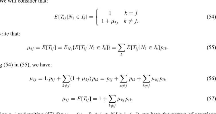
PROOF. We will consider that:

E[Ti j|N1∈ Ik] =

(

1 k = j

1+μk j k 6= j.

(54)

We can write that:

μi j = E[Ti j] = EN1{E[Ti j|N1∈ Ik]} = X

k

E[Ti j|N1∈ Ik]pi k. (55)

Replacing (54) in (55), we have:

μi j =1.pi j+

X

k6=j

(1+μk j)pi k = pi j +

X

k6=j

pi k +X

k6=j

μk jpi k (56)

μi j = E[Ti j] =1+

X

k6=j

μk jpi k. (57)

Establishing a j and writing (57) forμ = (μi j,0 ≤ i ≤ N I ei 6= j), we have the system of equations

given by:

(I−Q)μ=1. (58)

The Markov chain modeling can only be used together with a constant slaughter rate, and it is more appropriate for evaluation of scenarios in long-term planning. On the other hand, the Monte Carlo simulation approach can handle more general slaughter functions but it also requires a larger computational effort. A comparison between these two approaches, for constant slaugher rates is presented in the Results section.

RESULTS

In this study, we propose an evaluation of the growth of meat production in Brazil based on data regarding the number of cattle and annual slaughter between 1983 and 2008 (ANUALPEC 2008). The population and slaughter data referring to this period are presented on the graphs shown in Figures 1 and 2, in millions of heads, together with the adjusted values, according to the equations (3) and (5), respectively.

Table I presents the maximum likelihood estimates (MLE) and the standard deviation (SD) of the parameters of the Richards model adjusted to the population data in Figure 1, and of the parameters of the slaughter function adjusted to the data in Figure 2, as well as the 95% confidence interval forq

(14)

Fig. 1 – Bovine population in Brazil, in millions of heads, between 1983 and 2008.

Fig. 2 – Slaughter of the bovine population in Brazil between 1983 and 2008.

TABLE I

The MLE and SD estimates of the Richards model parameters.

Population

K q ρ τ−1

MLE 217.5701 3.4 0.1389 2.7642×10−4 SD 3.0419 1.554 0.01 7.9794×10−5

Intervention

φ0 φ1 R0 h0

MLE −0.0791 0.0019 42.1272 0.3294

(15)

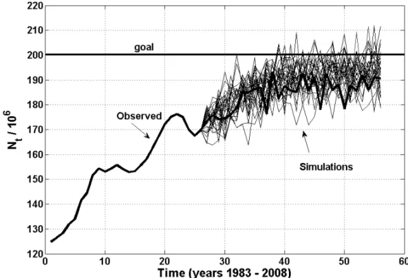
Fig. 3 – Simulation of the trajectories ofNt for 30 years ahead.

An important observation refers to the estimated values of K and h0 that represent the carrying

capacity and maximum slaughtering allowed, respectively. Note that the carrying capacity estimate

K =217.5701 exceeded the maximum population level N26 =176.1144 million head of cattle observed

in 2004 (see Figure 1) andh0 = 0.3294 that represents an estimate of the maximum slaughter rate that

is exceeding the maximum rate, which was about 0.2772, observed in 2006 (see Figure 2). K andh0

are the two main parameters that affect the population growth. In this work, we perform simulations of population growth for different values of K andh0, close to estimates values, in order to estimate the

probability and the expected time of the population to reach a given goal.

The graph in Figure 3 presents some of the 100 thousand simulations of trajectories of the process that were generated to calculate the probability of the population reaching the goal of 200 million heads.

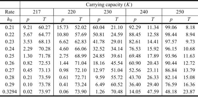
In Table II, we present the probability p (Percent) and the expected time T (year) for this event to

occur, considering scenarios withK increased from the estimated value to the value of 250 million heads,

andh0increased from the actual observed value 0.21 to the estimated value 0.3294 given in Table II.

Note that the probability that the Brazilian herd will reach the goal of 200 million head proposed by Pineda (2002) whenh0 =0.3294 andK =217 million heads is only p =0.02%, and the time expected

for this event to occur isT ≈74 years. These results point out that an optimized slaughter policy is needed, together with investments in technology that improve the reproduction rates and carrying capacity of the Brazilian bovine herd and make possible to reach the population goal in a desirable time interval asT ≈12 years withp ≈94%, which can be achieved with_h₀≈0.25 and K ≈250 million head.

COMPARISON BETWEEN THE MARKOV CHAIN MODEL AND MONTE CARLO SIMULATION

(16)

TABLE II

Indicators estimates via Monte Carlo simulation.

Carrying capacity (K)

Rate 217 220 230 240 250

h0 p T p T p T p T p T

0.21 9.21 60.27 15.73 52.02 60.04 21.10 92.29 11.34 99.06 8.18

0.22 5.67 64.77 10.80 57.69 50.81 24.59 88.45 12.58 98.44 8.94

0.23 3.53 68.13 6.62 62.83 41.78 29.01 82.61 14.41 97.57 9.73

0.24 2.29 70.28 4.60 66.06 32.52 34.14 76.53 15.92 96.15 10.68

0.25 1.30 71.78 2.75 68.99 24.85 39.61 69.48 17.89 93.96 11.63

0.26 0.82 72.53 1.44 71.04 18.16 45.54 60.90 20.43 90.44 12.72

0.27 0.45 73.13 0.98 72.10 12.97 51.04 52.56 23.11 86.84 13.79

0.28 0.21 73.59 0.61 72.71 9.59 55.72 43.70 26.33 82.14 15.08

0.29 0.10 73.78 0.41 73.24 6.49 60.52 36.40 29.40 76.59 16.36

0.3294 0.02 73.97 0.06 73.90 1.26 70.48 14.05 47.59 48.18 23.87

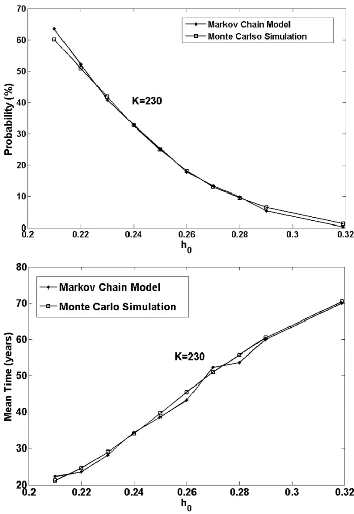
two methods we presented, in Figure 4, both indices calculated with each of the methodologies presented, considering K =230. Estimates made by the Monte Carlo simulation are in the third column of Table I.

An analysis of the curves in Figure 4 shows a great similarity between the two approaches. However, being practical, the modeling by Markov chain requires some careful with the choice of size and the discretization of the space state. These results can be seen in Table III and on the graphs in Figure 4.

TABLE III

Estimates of the indicators by Markov chain as function of maximum slaughter rate.

h0 Time-MC Prob-MC

0.21 22.2439 0.6340

0.22 23.5111 0.5211

0.23 28.1966 0.4079

0.24 34.4267 0.3279

0.25 38.6040 0.2514

0.26 43.2941 0.1775

0.27 52.3350 0.1333

0.28 53.6280 0.0983

0.29 60.0000 0.0537

0.30 T∞ 0.0135 0.3294 T∞ 0.0020

(17)

(18)

CONCLUSIONS

In this work, we presented the adjustment of the Richards growth model for the bovine population in Brazil taking into consideration the populational losses due to the slaughter intervention. With the model adjustment that includes the stochastic intervention and posteriorly Monte Carlo simulations, we were able to estimate the indicators of the population viability. By considering deterministic intervention, we calculated the indicators, assuming that the population can be modeled by a Markov chain. We also employed Monte Carlo simulations to compare the results between these two methods. The Markov chain model would be the most natural manner of obtaining estimates of a population viability indicators, but it depends on the discretization of the space of states. On the other hand, the method using Monte Carlo simulation requires the establishment of an upper limit that, in this work, we call T∞. This limitation may impair the accurate calculation of the time expected to reach the population goal.

The analysis of the numerical results shows that a slaughter rate higher than 25% can make the growth of the population difficult and, in the future, lead to the reduction of bovine meat production in Brazil. To reach a higher goal, such as 200 million heads in a period less than 20 years, an optimized slaughter policy is fundamental in order to maximize a certain expected return within a finite horizon.

Considering the stochastic intervention, we simulated 10 scenarios changing the maximum slaugh-ter rate and the carrying capacity, and concluded that the goal will be reached in 8 to 20 years (with

K = 250). This leads us to believe that the use of a fixed intervention equal to 25% (slaughter in 2005)

does not guarantee a sustainable production for K < 240. Given the present scenario, we can con-clude that the Brazilian bovine herd will not reach the goal of 200 million heads in the expected time of 15 years.

ACKNOWLEDGMENTS

Research partially supported by Fundação de Amparo à Pesquisa do Estado de São Paulo (FAPESP), Grant 07/007612-0 and by Conselho Nacional de Desenvolvimento Científico e Tecnológico (CNPq), Grant number 300235/2005-5.

RESUMO

Neste trabalho estudamos o problema de identificação do modelo de uma população utilizando um modelo dinâmico discreto baseado no modelo de crescimento de Richards. A população é submetida a intervenções devido ao consumo, como no caso de caça ou na criação de animais. A identificação do modelo permite-nos estimar a probabilidade ou o tempo médio de ocorrência para que se atinja um certo número populacional. A inferência paramétrica dos modelos é obtida através da técnica de perfil de máxima verossimilhança como desenvolvida neste trabalho. O método de identificação desenvolvido pode ser aplicado para avaliar a produtividade de criação animal ou o risco de extinção de uma população autóctone. Ele foi aplicado aos dados da população global de gado de corte bovino brasileiro, e é utilizado na investigação de a população atingir um certo número desejado de cabeças.

Palavras-chave: Modelo de crescimento de Richards, risco de populações, populações exploradas, estimação de

(19)

REFERENCES

AKÇAKAYA HR AND SJÖGREN-GULVE P. 2000. Population viability analysis in conservation planning: an

overview. Ecol Bull 48: 8–21.

ALLENLJSANDALLENEJ. 2003. A comparison of three different stochastic population models with regard to

persistence time, Theor Popul Biol 64: 439–449.

ANUALPEC. 2008. Anuário da Pecuária Brasileira (Annual of Brazilian Cattle, in Portuguese), Publisher FNP, 359 p.

BARNDORFF-NIELSENOEANDCOXDR. 1994. Inference and Asymptotics, Chapman & Hall, 360 p.

BOYCEMS. 1992. Population Viability Analysis. Annu Rev Ecol Syst 23(4): 481–506.

DERISORB, MAUNDERMNANDPEARSONWH. 2008. Incorporating covariates into fisheries stock assessment

models with application to Pacific herring. Ecological applications: a publication of the Ecol Soc Am 18(5): 1270–1286.

FITZHUGH JRHA. 1974. Analysis of growth curves and strategies for altering their shapes. J Anim Sci 42(4):

1036–1051.

FOWLERCW. 1981. Density Dependence as Related to Life History Strategy. Ecology 62: 602–610.

GILPINMEANDAYALAFJ. 1973. Global Model of Growth and Competition. Proc Nat Acad Sci 70(12): 3590–

3593.

JIAOY, HAYESCANDCORTÉSE. 2009. Hierarchical Bayesian approach for population dynamics modelling of

fish complexes without species-specific data. ICES J Mar Sci 66(2): 367–377.

LOIBELS, ANDRADEMGAND VALJBR. 2006. Inference for the Richards Growth Model Using Box and Cox

Transformation and Bootstrap Techniques. Ecol Model 191(3-4): 501–512.

LUDWIGD. 1996. Uncertainty and the Assessment of Extinction Probabilities. Ecol Appl 6(4): 1067–1076.

LUDWIGD. 1999. Is it meaningful to estimate a probability of extinction. Ecology 1(80): 298–310.

MATISJHANDKIFFETR. 2004. On Stochastic Logistic Population Growth Models With Immigration and Multiple Births. Theor Popul Biol 65: 89–104.

MATIS JH, KIFFETR, MATISTIAND STEVENSONDE. 2007. Stochastic modeling of aphid population growth

with nonlinear, power-law dynamics. Math Biosci 208: 469–494.

OMLINMANDREICHERTP. 1999. A Comparison of Techniques for the Estimation of Models Prediction Uncer-tainty. Ecol Model 115: 45–59.

PINEDANR. 2002. Cenário da cadeia Produtiva de Carne Bovina no Brasil. Revista da Associação Brasileira dos

Criadores de Zebuinos-ABCZ 2(10): 186–187.

POLANSKY L,DEVALPINE P, LLOYD-SMITHJO ANDGETZ WM. 2008. Parameter estimation in a generalized discrete-time model of density dependence. Theor Ecol 1: 221–229.

RICHARDSJF. 1959. A flexible growth function for empirical use. J Exp Bot 1(10): 290–310.

SAETHERBE, ENGEN S, LANDE R, ARCESE P ANDSMITH JNM. 2000. Estimating the time extinction in an

island population of song sparrow. Proc Roy Soc Lond 267(B): 621–626.

(20)

SAETHER BE, ENGEN S, FILL F, AANES R, SCHRODERW AND ANDERSEN R. 2002b. Stochastic population dynamics of an introduced swiss population of the Ibex. Ecology 83(12): 3457–3465.

SEBERGAFANDWILDCJ. 1989. Nonlinear Regression. J Wiley & Sons, 774 p.

SIBLY RM, BARKER D, DENHAM MC, HONE J AND PAGELM. 2005. On the Regulation of Populations of Mammals, Birds, Fish, and Insects, SCIENCE www.sciencemag.org. 309(22): 607–610.

YAMAUCHIA. 2000. Population Persistence Time Under Intermittent Control in Stochastic Environments. Theor