Work Project, presented as part of the requirements for the Award of a Master Degree in Finance from the NOVA – School of Business and Economics.
LIFE CYCLE MODEL AND HEALTH RISK
CONSTANÇA MARGARIDA PIMENTA PEREIRA DUARTE MARTINS (3965/24531)
A Project carried out on the Master in (Economics/Finance/Management) Program, under the supervision of: Fernando Anjos
1
Abstract
Life-cycle theory explains how an individual will allocate his wealth throughout his life. So far, research has been developed with empirical evidence diverging from model predictions. Recently, health has been introduced as a source of background risk but the main focus has been the retirement period. I will present here a simple model with health risk, showing how it impacts the choice of the young agent. I find that the wealthier and unhealthier the agent is, the less he will invest in the risky asset.
2
1. Introduction
Portfolio choice has always been a frequent issue in academic literature. Investigators have always been curious of the reasons why agents choose different portfolios in different times of their lives. From this curiosity, life-cycle models arose. Typically, these models maximize the agent utility given some wealth and consumption constraints. They aim to replicate the agent´s choices throughout his life and understand the factors behind his decision.
The early versions of these models would use simple preferences and would focus only in consumption and wealth accumulation decisions. The agent would also have two types of assets available, a risky and a safe one. At each point in time the agent can choose the allocation between these assets and consumption. Most recent models started introducing different variables, attempting to better replicate and explain the agent choice.
One factor that has only recently started being discussed is health. Until recently, models have ignored this factor. Nonetheless academics have been starting to acknowledge the relevance of this issue. Moreover health has impacts on many aspects of the agent life. When the agent becomes ill, he might not be able to work which affects his stream of income. If his illness becomes permanent, the agent will probably retire and die earlier. In addition, demographics have been changing. The population now lives longer than ever before. This means that the agent will have to save for a longer period after retirement not only to compensate for the drop in income but also to cover increasing medical expenses. Naturally, all of this will impact the agent choices regarding portfolio choice. Once it is understandable how all these factors move with each other, financial institutions can provide more customized financial packages to theirs clients.
3 Academics recently have been trying to address the issues mentioned above. Most of the work developed focus only on the period after retirement. It is in this period that most agents are faced with costly health choices. Moreover, most research done so far only focus on the choice between healthcare and consumption goods, ignoring the selection of financial assets.
This research aims to bring some clarity to this issue and understand how a young agent makes his portfolio choice today knowing he faces a health risk, retirement period, among other factors. Moreover, I want to understand how each individual factor will impact the agent decision.
In order to answer the questions above, I developed a model that determines the optimum percentage of wealth that the young agent should invest now, in the risky asset, to maximize his lifetime utility, given that he faces some health risks. The optimal allocation to the risky asset will change as I change the intensity of this risks. With this model, I will clarify how these parameters affect the agent decision. To develop this model, there was a need to understand which factors are relevant and how to apply them in this context.
The remainder if the paper is organized as follows. In section 2, I will analyze and highlight most academic work performed on this subject. In section 3, I will introduce the model, explain the variables and how I solved it. In section 4, I will present the results obtained. In section 5, I will present the interpretation of the results obtained in section 4. In section 6, I will conclude, presenting limitations and suggestions for further research. The probabilities used and numerical resolution can be found in the appendix.
4
2. Literature Review
The first models regarding life-cycle theory were provided by Merton (1969) and Samuelson (1969). In their studies they attempt to provide solutions to the problem of lifetime portfolio selection. These models were constructed under very restrictive conditions namely no labor income, assets returns are identically and independently distributed and markets are complete.
Before the work developed by these academics, most analysis regarding portfolio choice would only concern one period. Samuelson introduced one of the first models, where the agent takes into consideration all his lifetime (multiple periods of decision) when making decisions regarding consumption and financial investments.
The model developed was the starting point for many future models. The individual has a utility function dependent on consumption. He will want to maximize his utility, taking under consideration the duration of his life. He starts with some initial wealth and at his death age he will consume everything. There are two financial assets, one safe that always provides a constant return and a stochastic risky one that produces random returns. In order to solve this problem, the author uses dynamic programming. Samuelson starts in the last period where the agent consumes everything and there is no financial decision, becoming a single period problem. Solving this, the decision in the period before can be easily calculated since it is known what happens in the future. The problem can be recursively solved until arrival to period 0.
It is important to reinforce that the results of this model were obtained under severe constraints. The author suggests that by using other utility function (in this model a constant relative risk-aversion function is used), that is, if the elasticity of marginal utility rose with wealth (higher wealth, higher risk-tolerance), the young agent might have
5 actually increased his risk tolerance after accumulating some wealth over the years. The model also does not considers labor income or other factors that could change this outcome.
Later, Bodie, Merton and Samuelson (1992) present a model concerning the introduction of labor supply flexibility. With this research, they want to investigate how labor and investment are connected. The main idea is that the agent can adapt his work supply based on his financial outcomes. For example, a younger agent can perform more risky investments since, even if the investment goes wrong, he can work harder in the future and compensate this loss.
This paper highlights the role of human capital in life-cycle models. Although not tested empirically, the author suggests several relevant hypotheses. For instance, the agent will reduce his risky investments as he nears retirement, in this case supported by the argument that as the agent grows older he will have less labor flexibility. It is central to keep in mind that in real world most agents do not have complete flexibility regarding labor supply and cannot chose the amount of labor they will supply in each period.
Once established the relevance of labor and income, academics could focus on developing a realistic model that takes into consideration all this features. Cocco, Gomes and Maenhout (2005) derived a complete model featuring all of these parameters. I will be using a simplified version of this model. The model will focus on how an agent chooses the optimal portfolio choice when he faces labor income risk, mortality risk, uncertainty regarding retirement income, bequest motive and recursive preferences. There are two financial assets, one safe and one risky. The risky asset will be correlated to the permanent labor income. The agent can borrow or short-sale with some constraints. The problem is solved using backward induction. Once more the author starts at the end and derivate the conditions until arrival to period 0.
6 Concerning retirement, the authors explain that since future retirement income will be a constant, it will act as a substitute for the risk-free asset. Consequently, the investor will invest more in the risky asset the higher the retirement income. Moreover, an individual with small wealth will take a more risky position since his allocation to the riskless asset (future retirement income) is relatively bigger than the ones with higher initial wealth.
Similarly, the labor income also behaves as riskless asset since it is not highly correlated with the stock returns. In the previous model risky asset returns and labor income were perfectly correlated, which made labor income more similar to the risky asset rather than the riskless one. An interest result was that in fact the present discounted value of labor income must rise with age. This means that the agent will invest more in the risky asset as he ages. This is explained by the fact that in the beginning of his life the agent has a low labor income that will increase with age.
Analyzing their benchmark case, in the beginning agents will choose to only hold the risky asset and as they age, they will shift towards the riskless asset. Overall, the presence of labor income in the model will lead to a higher allocation to the risky asset. However, when the possibility of disastrous income is added it decreases the allocation.
Although all these models are becoming more complete and representative of the typical investor in reality young agents do not invest a high percentage of their wealth in the risky asset as the models predicted. Furthermore most families do not even hold any risky assets.
So far I have seen that it is important to include different factors namely labor income in order to achieve more realistic results. Moreover even though most models recommend a high allocation to the risky asset when agents are young this does not happen in reality.
7 Most models defend that the agent should take higher risks when young since he will have time to recover those losses and he can expect higher income in the future. A different approach is taken by Benzoni, Collin-Dufresne and Goldstein (2007). In their paper they prove that when the stock and labor market are cointegrated the agent will invest less in the risky asset when young, matching the empirical observation.
As mentioned previously when labor income is introduced the agent should take more risk since he can expect a more or less constant stream of income in the future. The innovation brought by these authors is that labor income will be cointegrated with the dividend process. Once more dynamic programming is used to solve the problem.
When taking this assumption, the allocation to the risky asset will be hump shaped. When the agent is young he will invest little or even take a short position in the market. As he ages the allocation will increase till a certain point where it starts decreasing. This is easily explained. When the investor is young, his wealth is highly dependent on future income that is highly correlated with market returns. Therefore the agent is already exposed to risk. Having an implicit exposition to risk, the agent will invest in riskless assets. When the agent grows older, the agent is less exposed to the risk of future income and will need to start investing more in the risky asset to achieve his optimal allocation. As death gets closer the cointegration factor has less time to act and future labor income becomes riskless. In the presence of asset return predictability, the results are consistent.
Furthermore, it was found that for a young agent the correlation between stock returns and returns from human capital (measured by future labor income) is around 50% and will be constant through the first half of the agent’s life. But as he grows older it gets to zero reasonably fast.
8 To this point it was discussed how to solve life-cycle models and what factors to incorporate. It was established the importance of labor income and how other factors can impact the outcome of the model.
One of the factors that has become more relevant is health. In the recent years numerous academics have researched the relevance of health when the agent chooses the portfolio. The results are ambiguous, while some conclude that health is a determinant factor, others defend that health is not at all relevant.
Rosen and Wu (2003) analyze the role of health, by examining a data set of retirement agents’ portfolio decisions. In this study, the agents would self-report their level of health. The authors show that just by having poor health the agent has a lower probability of owning financial assets. An interesting outcome of this study was that health does not seem to influence the individual attitude towards risk that is, being sick does not induce the agent to be more risk averse. Furthermore it would be expected that healthy and less healthy individuals portfolios would differ based on their horizon of life perspective. However the authors found no evidence of this. Even when considering bequest motives or health insurance, these mechanisms do not justify the conclusion drawn above. One explanation considered is that health can affect expectations of future income and therefore portfolio choice.
Overall poor health is associated with a lower probability of holding financial assets. Even if the individuals hold financial assets these are typically the safe type. Agents with poor health are less able to adjust their labor supply in case of bad financial perform and therefore prefer safe assets.
Consistent with previous results, Bressan, Pace and Pelizzon (2104) determine that is the self-reported status of health that affects portfolio choice and not health itself. When
9 the agent believes he is ill, he will reduce is allocation to the risky asset since he believes that he will incur in medical expenses or die younger. The study uses 3 measures of health: self-perceived, objective health and mental health. Only the first is statistically significant.
In general, most empirical studies conclude that health, in general, is not very significant when the individual is choosing his portfolio. However there is a positive correlation between health and holding financial health. Moreover when considering self-perceived health, health becomes a relevant factor as a source of background risk.
Now that a relationship has been established between health and portfolio choice I will discuss how academics have been modelling this relation. Most models so far focused on the post retirement period, since this is the period where agents are most concerned with their health and are most likely to suffer health shocks. Moreover with the increased pressure on the insurance companies, some models attempt to incorporate medical insurance as part of their model.
The first model I am going to analyze is from Hugonnier, Pelgrin and St-Amour (2012). Before, models had exhibited health and financial choices as separated decisions, this is one of the first models that joins the two factors. This paper provides a model that jointly determines consumption, portfolio choice, health investment and insurance coverage. Their model is based on the early Merton model.
Initially, the agent has recursive preferences and faces mortality and morbidity risks. These risks are partially controllable. The agent faces surviving probabilities that can be increased if the agent invests in his health and can decrease in the presence of an exogenous health shock (e.g. cancer). Moreover health investments have a bigger impact
10 when the agent is ill. This is a very realistic feature since, when the agents are healthy and go to the doctor they do not become healthier.
The labor income will be a function of his current health status. The author explains that an unhealthy agent will skip more days of work so he will receive a lower wage. Furthermore, it will only be affected by health shocks.
There are two financial assets, a riskless bond and a risky stock. Additionally the agent can invest in health through a health insurance contract. The authors assume that the agent is aware of his health status and can purchase this health contract (foregoing one unit of consumption) every period. The agent can choose the amount of coverage.
In this model the health will be incorporate not only in the utility function as a risk parameter (better health, lower morbidity and mortality risk) but also through the budget constraint (better health, higher income).
The authors test the model empirically. Consumption is increasing in health and wealth, as well as stock holding. An interesting result is that even if the agent is poor, as long as he is healthy the model predicts high investments in the risky asset. As expected as wealth increases the level of health insurance also moves in the same direction. The actual level of coverage in real life was lower than the one estimated. This is explained by employer coverage that is not covered in the model.
Furthermore, investment in the risky asset and life expectancy increase with agent’s health and longevity is independent of wealth. Moreover, stock holding and life expectancy are positively correlated. Overall, the model is consistent with the empirical data.
11 As mentioned previously, self-perceived health plays a relevant role in portfolio choice. Edwards (2008), will investigate this fact by focusing on the elderly individuals who usually perceive health as risky and reduce risky asset allocation.
The outcome of the study is in line with previous conclusions. Elderly people perceive their health as more risky, and to hedge it, they shift their portfolio toward safer assets. The author believes the medical expenditure risk is the main reason of this type of behavior. Furthermore the presence of health in the utility function seems relevant. When the agent is unhealthy, he will not be able to perform some activities he was able before and will be required to pay for those activities, for example, cooking or driving. Even when the agent has health insurance, this usually only covers some services and medical expenses. If health insurance was just money paid to the agent than this could hedge the risk.
More recently, Yogo (2016) focus on health risk and how this affects consumption, health expenditure and portfolio allocation in the retirement period. The addition of this paper to the previous literature is that housing is also included. Many of these factors have been studied individually but never all together in the same model.
The model starts at retirement. At this point in life, the retiree has a certain amount of wealth, housing wealth and health. Every period the agent suffers stochastic depreciation of health that affect consumption and life expectancy. Moreover, the agent receives income every period. After this the individual chooses consumption, health expenditure, portfolio allocation and housing expenditure.
Concerning housing, the agent faces a stock of housing that depreciates every period at a constant rate. After the depreciation the agent can choose to increase or decrease (e.g. downsizing) his position on the housing situation. Housing has a saving purpose, at any
12 time the agent can disinvest and use the money for consumption or health expenditures. Additionally, the agent gains utility from having a home. In real life, agents do not make housing decisions every period since this would be too costly.
As previously, the agent has a stock of heath that faces depreciation. This depreciation is now stochastic and depends on the agent´s characteristics. The agent dies when the stock of health reaches zero. Health expenditure impact lasts more than one period and there is no possibility for disinvesting. As in some previous models, health is subject to diminishing returns, that is, when the agent is ill, investing in health has a larger impact.
Once again there are two types of financial assets, bonds and stocks. Bond are the safe asset with a fix return. Stocks are the risky asset with random return. Housing stock also has a stochastic growth rate of return.
After solving and calibrating the model the author concludes that as expected the holding of the risky asset is low across retirees and is related to health status. This relationship is more significant for young retirees.
13
3. The model
The model starts at the current age of the agent. Every period is denoted by t and the agent lives for a maximum of T periods.The investor only works during a certain amount of periods, determined by the retirement age. The retirement age is exogenous. The agent has constant relative risk aversion (CRRA) preferences,
𝑢(𝑐
𝑡) =
𝑐𝑡 1−𝛾1−𝛾
(1)
where 𝑐𝑡 represents consumption at time t and 𝛾 is the level of risk aversion. This type of preferences were selected since they facilitate calculations. The percentage of consumption and level of risk aversion are always positive. There is no bequest motive since, as mentioned in the chapter before, this factor is not very relevant for the young investor.
Every period t there is a probability that the agent dies. These probabilities were set accordingly to the data of Social Security Administration of US for male individuals and will be influenced by a health risk (appendix 1).When the agent is ill, the probability of dying increases. This increase only lasts one period. This process will determine the death age of the agent.
While the agent is working, he receives an exogenous amount of income. This income grows at rate 𝑟𝑤,𝑡 , with mean 𝜇𝑤 and volatility 𝜎𝑤:
𝑤𝑡+1 = 𝑤𝑡∗ (1 + 𝜇𝑤± 𝜎𝑤) (2) After retirement the agent will start receiving a constant amount of income,
14 There are two types of financial assets in which the agent can invest. The risk-free asset that provides a constant return of 𝑟𝑓 every period and a risky asset that provide a
return of 𝑟𝑚,𝑡 every period. The return of the risky asset has a mean of 𝜇𝑚and a volatility of 𝜎𝑚. The agent cannot short-sell or leverage. The borrowing constraint assures that the investor will not have a negative allocation in the riskless asset and that he will not borrow against future labor or retirement income. Assuming 𝛼𝑡 denotes the percentage invested in the risky asset at time t, these restrictions guarantee 0 ≤ 𝛼𝑡 ≤ 1.
Moreover there is a health risk. Every period there is a probability that the agent will get ill. These probabilities are exogenously determined and increase with age. If the agent gets ill in period t, the agent increases his death probability and suffers an income reduction in period t. This reduction will be determined as a percentage of labor income. This only applies to the period where the agent is working and receives labor income and not in the retirement period, since it was mentioned in the previous chapter that this random income shocks has little impact to the young investor when it happens in the retirement period.
Every period t the investor receives labor income 𝑤𝑡. At period t, the agent will have
a wealth of 𝑥𝑡, that includes initial wealth plus labor income. After this the agent will
decide his optimal allocations. The agent will consume 𝑐𝑡, and allocate the remaining between the risky and riskless asset. 𝑅𝑡+1𝑝 is the return of the portfolio selected in the previous period,
𝑅𝑡+1𝑝 = 𝛼𝑡𝑟𝑚,𝑡+ (1 − 𝛼𝑡)𝑟𝑓. (3)
The individual will maximize his preferences subject to the constraints mentioned above. The control variables of the problem are {𝐶𝑡,𝛼𝑡}𝑡=1𝑇 and the state variables are
15 {𝑡, 𝑥𝑡, 𝑣𝑡}𝑡=1𝑇 . Our goal is to obtain the optimal consumption and the portfolio choice,
regarding risky and riskless asset.
The value function is homogeneous with respect to labor income. The Bellman equation for this problem is given by,
𝑉𝑡(𝑥𝑡) = max
{𝑐𝑡,𝛼𝑡}
[𝑈 (𝑐𝑡) + 𝛽𝐸𝑡𝑉𝑡+1(𝑥𝑡+1)] (4)
where β is the discount factor and,
𝑥𝑡+1 = 𝑤𝑡+1+ (𝑥𝑡− 𝑐𝑡)(𝛼𝑡𝑟𝑚,𝑡+ (1 − 𝛼𝑡)𝑟𝑓). (5) In order to solve this model I will used backward induction and derived the solution
numerically. Since there is no bequest movie, in the last period, the agent will consume all his available wealth and there is no financial decision. Having the last period solve I can substitute this value in the Bellman and solve for the previous period. I use this strategy, until I arrive to period 0. I optimize the solution by using grid search.
Most parameters are in line with Cocco, Gomes and Maenhout (2005). The discount factor is given by,
𝛽 = 1
1 + 𝑟𝑓
(6)
and the risk-free rate is set to 2.00%.
The mean equity premium is 4.00% with a standard deviation of 15.00%. Regarding wage, the mean is 2.00% with a standard deviation of 3.00%. All the other parameters are explained in the next chapter.
16
4. Results
I will start with the baseline model and then introduce some different parameters and see how the model reacts. For every different parameter and for the baseline model 50 portfolio choices were calculated. For every calculation, I will save the initial risky asset allocation chosen by the young investor. I will focus on the young agent and how his decision changes when I change some of the parameters. The parameters mentioned in the chapter above will be fixed throughout this analysis.
4.1 Baseline Model
For the baseline model I will assume that the agent is currently 25 years and possesses a wealth of 2. The labor income growth will be correlated with the risky asset returns. This correlation will be of 0.2. The agent will have a risk aversion (𝛾) of 10. Retirement age will be 65. The agent has a probability of getting sick that starts at 5.00% and increases by 5.00% every 10 years. Moreover, every time the agent gets sick, he increases his probability of dying by 1.00%. When the agent is ill he only receives 50% of his normal wage. When the agent retires he receives a fix income of 2. Usually the retirement income is fixed as a percentage of the last salary received but for easiness of calculations, a fixed exogenous value was selected. I report the values obtained with the model for alpha for the investor below.
Alpha Mean 29,25% St. Dev. 7,45%
Max 38,38% Min 19,19%
17 On average, the agent will invest 29.25% of his wealth in the risky asset. However I can see there is some dispersion. In the table below I plot the alpha and the correspondent death age.
In general, the risky asset allocation is increasing with death age, the later the agent dies the more he invests in the risky asset. This result is in line with previous studies. Additionally, it appears that this increase is steeper for younger ages of death and from a certain death age on the alpha allocation does not increase, for example, if the agent dies at 50 instead of 40 this increases his allocation to the risky asset significantly however I consider 80 instead of 70 there seems to be no significant differences. It appears that from a certain death age, adding more years of life do not imply higher risky asset allocation.
4.2 Correlation between wage growth and risky asset returns
In this section I will see how the agent changes his risky asset allocation when the two parameters above are not correlated and when this correlation is strong. As I mentioned before, this correlation will depend on many parameters not considered here. The correlation is denoted by parameter 𝜌. In the first case I will assume a correlation of
0 0,05 0,1 0,15 0,2 0,25 0,3 0,35 0,4 0,45 25 26 28 29 31 31 33 36 38 40 43 53 56 57 68 71 79 alp h a death age
Death age and Alpha allocation
18 0 and in the second case I will assume a correlation of 0.4. All of this correlations chosen are very conservative regarding empirical evidence. The results are reported below.
From this table I can conclude that correlation plays a huge role in the risky asset allocation. As the correlation increases the percentage allocated decreases dramatically. Moreover the dispersion decreases when the correlation increases.
4.3 Initial wealth
The initial wealth is measured in the model as the ratio between current wage and wealth divided by the current wage. Therefore this value has to be at least 1. I will test 2 different cases. One where the agent has no wealth and will only receive labor income which means a value of 1. The other case will be of when the agent is already quite wealthy, represented by a value of 5.
Alpha 1 2 5 Mean 91,25% 29,25% 16,02% St. Dev. 12,78% 7,45% 3,18% Max 100,00% 38,38% 22,22% Min 65,66% 19,19% 12,12% Table 3- Risky asset allocation - initial wealth
As in the previous case I get extreme results. When the agent is poorer, he will allocate on average 91.25% of his wealth to the risky asset. This allocation is very disperse. This is an interesting result but since it would be expected that a less wealthy agent would be
Alpha 0 0.2 0.4 Mean 42,79% 29,25% 14,26% St. Dev. 11,71% 7,45% 1,59% Max 61,62% 38,38% 16,16% Min 27,27% 19,19% 11,11%
19 safer and invest more in the risky asset. As I increase the level of wealth the results become less disperse and the allocation to the risky asset drops dramatically. A slight change from 1 to 2 decreases the average allocation to 29.25%. It seems that wealthier agents are less inclined to invest in the risky asset. It seems wealth has more of an impact when the agent is poor.
4.4 Risk aversion
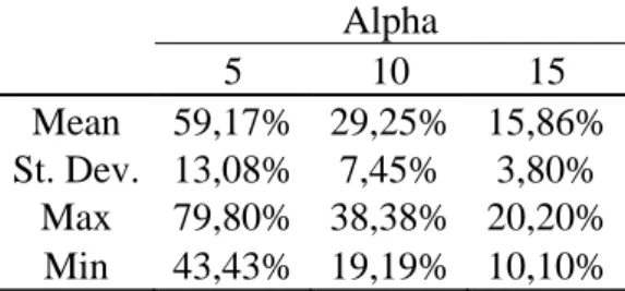
The risk aversion parameter measures the willingness of the agent to engage in risky behavior. As a baseline I assume a value of 10 consistent with previous studies and usually considered quite risk-averse. I will consider other 2 levels of risk aversion. The first where the agent is risk-lover with a value of 5 and the case of a safer agent with a value of risk aversion of 15.
Alpha 5 10 15 Mean 59,17% 29,25% 15,86% St. Dev. 13,08% 7,45% 3,80% Max 79,80% 38,38% 20,20% Min 43,43% 19,19% 10,10% Table 4: Risky asset allocation - risk aversion
As expected the agents with the lower risk aversion will allocate more wealth to the risky asset. This case also has a higher standard deviation. As the level of risk aversion increases the percentage allocated to the risky asset decreases as well as the dispersion of the results.
20
4.5 Initial age
The initial age of the agent is very important. This will determine the lifespan of the agent. The earlier the agent starts investing the more time he will have to recover from losses among other factors. I will consider 2 cases where the agent is older, in one the agent will be 35 and the other 45.It is important to have in mind that older agents usually are more risk averse and have a higher ratio of wealth accumulated than younger agents. When the simulation is done, only the age will change. The results are reported in the table below.
The results show that against what was predicted, the initial age does not seem to play a relevant role in risky asset allocation. As I increase the age there is a slight decrease in the average allocation as well as in the dispersion of the results. The lowest allocation simulation was the same in all the 3 cases.
4.6 Retirement age
The retirement age determines the moment where the agent starts receiving the fixed income. The earlier the agent retires, the earlier he starts receiving a fixed amount of income. The impact of this parameter depends on how different the labor income differs from retire income. I considered an earlier retirement age of 60 and later of 70.
Alpha 25 35 45 Mean 29,25% 28,32% 27,09% St. Dev. 7,45% 6,13% 5,46% Max 38,38% 36,36% 33,33% Min 19,19% 19,19% 19,19%
21
In general there are no relevant differences between the 3 cases. As I increase the age of retirement the risky asset allocation slightly increases as well as dispersion. It appears the later the agent retires the more he will invest in the risky asset.
4.7 Retirement wage
The retirement income plays a relevant role in the life-cycle model since it represents a constant stream of income that the agent has for certain in the future. However the impact of this income depends on it compares to the wage earned previously and the wealth accumulated until then. I will consider a lower retirement income of 1 and higher income of 4. The results are reported in the table below.
When the agent has a lower retirement income he will on average invest a slightly higher amount on the risky asset. The alpha associated with the higher retirement income does not differ significantly from the alpha associated with the middle income which suggests that from a certain threshold on, higher income will not translate into a lower risky asset allocation. All the cases present similar dispersions.
Alpha 60 65 70 Mean 28,83% 29,25% 29,66% St. Dev. 6,94% 7,45% 8,19% Max 38,38% 38,38% 39,39% Min 19,19% 19,19% 15,15% Table 6: Risky asset allocation - retirement age
Alpha 1 2 4 Mean 31,60% 29,25% 29,60% St. Dev. 6,60% 7,45% 6,68% Max 42,42% 38,38% 38,38% Min 19,19% 19,19% 19,19% Table 6: Risky asset allocation - retirement wage
22
4.8 Probability of illness
Every period there is a chance that the agent will get ill. As mentioned previously for our baseline case, this probability starts at 5% and increases by 5% every 10 years. Not every agent has the same likeliness of getting ill. In this sub-chapter I will consider 2 different cases. The first in where the agent has a lower probability of getting ill, denominated by L and the other where the agent has a higher probability of getting ill, denominated by H. The N represents the normal likeliness of becoming ill used in the baseline case.
When the agent has lower probabilities of getting ill, he will on average allocate more wealth to the risky asset. Moreover when the agent has higher probabilities of getting ill, he will decrease his allocation to the risky asset. On all 3 cases the maximum value and the minimum value allocated to the risky asset is the same.
4.9 Wage when ill
When the agent is ill he will suffer a reduction in income. In the baseline case, I assumed a reduction of 50.00%. As before there are situations where the agent is so ill or the medical expenses are so high that the agent will receive no income or it can be a light shock where the agent receives most of income. I will consider here 2 situations, one where the agent receives 0.00% of income and another where the agent receives 75.00% of income when ill.
Alpha L N H Mean 30,65% 29,25% 27,31% St. Dev. 6,79% 7,45% 7,33% Max 38,38% 38,38% 38,38% Min 19,19% 19,19% 19,19% Table 8: Risky asset allocation – probability of illness
23 When the agent is ill with 0 income he will reduce is risky asset allocation to 23.09%. The unexpected outcome arises when I consider a reduction in income of only 25.00%. In this case the average risky asset allocation dropped to 27.11% comparing to the baseline case.
4.10 Probability of dying when ill
When the agent becomes ill, this is going to increase the probability of dying in that period. In our baseline case I assumed an increase of 1%. In here, I will consider other 2 cases, an increase of 0.5% and of 5%. The higher the increase, the higher the likelihood that the agent will die earlier.
As expected when I decrease the probability to 0.5% the agent will invest more in the risky asset since he will more likely live longer and when I increased the probability to 5% the agent decreases this allocation corresponding to the higher likelihood of dying earlier. Alpha 0% 50% 75% Mean 23,09% 29,25% 27,11% St. Dev. 14,15% 7,45% 7,57% Max 38,38% 38,38% 38,38% Min 0,00% 19,19% 19,19% Table 9: Risky asset allocation – wage when ill
Alpha 0.5% 1% 5% Mean 31,64% 29,25% 22,30% St. Dev. 6,95% 7,45% 4,53% Max 38,38% 38,38% 38,38% Min 19,19% 19,19% 19,19% Table 10: Risky asset allocation – probability of dying when ill
24
5. Discussion
A young agent in the beginning of his life, with some wealth and some risk aversion will invest around 30.00% of his wealth in the risky asset. However from the results obtained, the maximum amount allocated was close to 40.00% and the minimum to 20.00% suggesting some heterogeneity among the individuals.
When I compare average risky asset allocation with the individuals’ death age I can see that the later the agent dies, the higher the risky asset allocation is going to be. When the agent lives for more periods he will receive more income, which translates into an implicit holding of the safe asset making the agent more prone to take risk. Furthermore, living longer implies an extended period receiving a constant, non-risky stream of income.
As mentioned before there is some evidence of correlation between market returns and wage growth. It is expected that when the market is strong there will be a positive growth in wages. Studies show this correlation can be near 50 % for a young agent and tend to decrease later in life. In the previous chapter, I observed that as I reduced the correlation the risky asset allocation, the risky asset allocation increases. This can be easily explained. When the investor understands that his wage has some degree of correlation with the market, he will want to reduce his exposure. By receiving his wage, he is already exposed to some level of market risk, so as this correlation increases the agent will want to reduce even more his risky asset allocation.
An investor in the beginning of his life, usually does not have a large amount of wealth. However there are agents that at a young age already possess a considerable amount of health. When this hypothesis was tested, I obtained surprising results. It would be expected that if the agent has less initial wealth, he would be more risk averse since he
25 does not have a lot of wealth to compensate for future losses. However I obtained different results. When I reduced the initial wealth to the minimum of 1, the average allocation to the risky asset increased to 91.25%. On the other hand, when I increased initial wealth, the average allocation decreased to 16.02%. I believe that since the agent is at a level of such little wealth, that he prefers to invest more aggressively in order to raise his wealth instead of playing it safe. On the other case, the agent is already so rich that he has no incentives to take on more risk. Moreover the agent who has little wealth now, has relatively more future wealth (retirement income). Having a higher relative future health, this represents also a higher implicit investment in the riskless asset. This could explain why the less wealthy agents invest more in the risky asset.
In our baseline case I considered a risk aversion of 10, considered by many authors already a high level of risk aversion. The level of risk aversion measures the preference of the agent regarding risky investments. Therefore it can be expected that a higher level of risk aversion translates into a lower risky asset allocation. The results obtained were in line with the expectations.
Regarding initial age, one would thought this parameter was of high relevant since it defines how many periods the agent will live. I considered 2 older agents with 35 and other with 45 years old. The 3 cases do not present relevant differences. This parameter would probably have more impact if it was more consistent with other parameters. Older agents are usually more risk averse, have a higher level of wealth accumulated. If these parameters had changed accordingly, the results would probably be more relevant. Overall, the standard deviation also decreases as the initial age of the investor gets bigger.
Another relevant parameter is the retirement age, this parameter determines how many periods the agent receives labor income and how many periods the agent receives a non-risky income. One would expect that the lower the retirement age, the longer the
26 individual receives a constant stream of income, that will translate into a higher risky asset allocation. However if the retirement income his lower than current wage, the younger the agent retires, he can expect to have more periods receiving a lower income and this would induce a lower allocation to the risky asset. Although all 3 cases considered (60, 65 and 70 years old) do not present relevant differences I can observe that as I increased retirement age the risky asset allocation increased. This results are consistent with the second explanation. I considered the same retirement wage independently of age of retirement. In fact, the later the agent retires, the less retirement income he will receive. Moreover, in real life, people have some choice of when they want to retire. If I had introduce this factors, I could have observed more differences in the risky asset allocation.
Concerning, retirement wage, this defines the non-risky amount of income that the agent receives after retirement. Since the retirement wage is constant, one would expect that the higher the retirement income, the higher the risky asset allocation. The agent would be able to recover from future losses with this income. However this does not seem to be the case. When the individual receives a lower retirement income of 1, he invests more in the risky asset than in the baseline case where he receives 2. Moreover when I increase the retirement income to 4, the agent also increases his risky asset allocation when comparing to the baseline case. It seems there are 2 forces in action. I believe that when the agent expects to receive a low retirement income, he will invest now a higher percentage in the risky asset in order to accumulate wealth to compensate for the low income later. When the agent expects to receive a high income in retirement, he has incentives to take more risks and he will invest more in the risky asset, since he does not need to accumulate so much wealth for retirement. Moreover even if he suffer some losses he can compensate with retirement income.
27 There is a chance that the agent will get ill every period. This probability is exogenously determined and is increasing in age. When the agent becomes ill he suffers a reduction in income and increases his probability of dying. Given this, I can expect that when I increase the probability of getting ill, the risky asset allocation will decrease. This is indeed true. The young agent, expecting some future losses in income and an increase probability of dying, will take a safer approach and decrease his allocation to the risky asset.
When the agent is ill, this will affect his income. This reduction in income represents an inability to work or the payment of medical expenses. In the baseline case I assumed a reduction of 50%, and later I consider two other cases where the agent receives no income at all and another where the agent only suffers a 25.00% reduction.
It would be expected that as I increase income, the agent would increase his allocation to the risky asset. The results are consistent with this prediction. When I introduce the 0 income case, the average allocation dropped from 29.25% to 23.09%. However, I would expect that when I increase the income to 75.00% the average risky asset allocation would increase. In fact, the allocation dropped to 27.11%. This result is very puzzling.
The last thing to consider is the increase in the probability of dying when the agent is ill. As expected, when increased the probability of dying the average risky asset allocation dropped. Since the agent expects a shorter life, he will prefer to consume more and invest in the safe asset than investing in the risky asset. Furthermore, when I decrease the probability to 0.05%, the average allocation increased.
28
6. Conclusion
In this research, I developed a life-cycle model that solves for optimal portfolio allocation. This model features an agent that is the beginning of his life, 25 years old, and has to decide how much to invest in the risky asset now, giving all the uncertainty from the future. This individual has some wealth and receives uncertain labor income. Moreover the labor income is correlated with risky asset returns. Most of the results are in line with previous studies however there were some puzzling outcomes.
The correlation between the risky asset returns and wage growth seems to be relevant in life-cycle models. The bigger the correlation, the smaller the allocation. If the market returns are indeed correlated with wage growth this can help explain why the young agents are not investing. Furthermore, when the agents are young are more dependent on wage, since they do not possess much wealth. The wage will act as a substitute of the risky asset, and the young agent has already an implicit position in the market. It is important to further study this relation and establish how strong it is.
A surprising outcome arose from the initial wealth parameter. The results showed that the poorer the agent, the more he would invest in the risky asset. This fact goes against empirical evidence. When the agents are poor they tend to behave more safely, that is, knowing he does not have much wealth he would invest more in the safe asset. The model results tell us otherwise, since the agents with barely any wealth will invest almost all of it in the risky asset. An explanation could be that the future income will act as a riskless asset meaning that poorer agents have a higher implicit investment in the riskless asset already giving him more incentives to invest in the risky asset. Further research would have to be done in order to understand the true mechanisms behind this result.
I also examined the initial age and retirement age. The initial age does not seem to have a large impact in the risky asset allocation. The baseline parameters were set for
29 a younger agent so when considering an older agent, the parameters should have been set accordingly. Regarding retirement age, I obtained some unexpected results. According to the model when the retirement age increases, the risky asset allocation increases. Usually, if the agent retires earlier, he would receive a constant stream of income for a longer period what would induce him to take more risk. This result can be induced by a low retirement wage. If the agent is receiving a high wage before he retires, the longer he stays working, the higher income he receives and the more he will chose the risky asset. This is consistent with the fact that higher retirement age has a higher allocation.
Concerning retirement income, the results were also surprising. The lower the retirement wage, the higher the allocation to the risky asset. It seems that the young agent perceiving that he will not earn enough money in retirement, he allocates more to the risky asset in hope to increase his wealth now to compensate for the retirement period.
In terms of health, the higher the probability of getting ill the lower the risky asset allocation. This result was expected, since this has implications in the individuals’ income. The chance of a lower income induces the agent to act in a safer manner. Also, the probability of getting ill has implication in the length of the agents’ life. When I increased this probability, the risky asset allocation dropped what was expected. I obtained an interesting outcome when considering income when the agent is ill. In the baseline case I considered a 50.00% reduction in income, and when I reduce the income to 0, the average risky asset allocation dropped. However when I decreased to only a 25.00% reduction, the average location decreased comparing to the baseline case. Further research needs to be done to find the reason for such odd outcome.
With this research I brought some light to the behavior of the young agent regarding his portfolio allocation. Moreover I showed how health impacts this decision. Additionally, this study can de proven useful to financial institutions. This simple model
30 gives an indication of what the agent should invest now. Once calibrated to each costumer, the institutions can provide more customized solutions.
In here I present a simple model. The limitations arise from its simplicity. In the model, the young agent knows some information about the future. To present a more solid realistic model, I would have to add new parameters or make the present ones more realistic. For example, every time there is a health shock, the probability of dying only increases in the period. The shock could be made more permanent, having an impact in all future periods. Or I could have two types of illness, one temporary that only impacts that period and a chronic one that would last more than one period. Moreover, in this model a health shock affects income directly. In the real word, people have insurance and usually do not suffer such a dramatic income shock. There could be some form of insurance in the model, such that the agent would choose between consumption, financial assets and health insurance. If the agent purchase health insurance then the labor income shock would not be so drastic. Additionally health could be a source of utility. The agent gains utility from being healthy, that is, when purchasing insurance the agent is increasing is utility.
Furthermore, I impose a retirement age. In real life, people decide when to stop working. The retirement age could be an endogenous parameter dependent on the health, wealth accumulated and labor income. For example, if the agent is very unhealthy or he already accumulated enough wealth he might choose to retire early.
Concerning the utility function, I used a very simple constant relative risk aversion function. A more complete version of this model could be obtained by using recursive preferences. A sub-type of this preferences that could be relevant in this context is Chew-Dekel preferences. In this case, the agent is more sensitive to bad events. There is a risk aggregator that defines preferences. There is also a certainty equivalent, if the event is
31 above the certainty equivalent it is good, if the event is below the certainty equivalent it is bad. This type of utility preferences puts additional weight in the bad outcomes such that the agent has disappointment aversion.
Another type of recursive preferences more commonly used are Epstein-Zin preferences. In here, there is not only a coefficient of risk aversion but also a coefficient for elasticity of intertemporal substitution. In this type of utility functions the agent can show his preferences regarding uncertainty. If the agent dislikes uncertainty, as most agents do, he will prefer early resolution. The utility function used in the model is a special form of this one.
32
Appendix
1. Death Probabilities and Health Probabilities
AGE DEATH PROBABILITY N L H
0 0,63830% 5,00% 0,00% 10,00% 1 0,04530% 5,00% 0,00% 10,00% 2 0,02820% 5,00% 0,00% 10,00% 3 0,02300% 5,00% 0,00% 10,00% 4 0,01690% 5,00% 0,00% 10,00% 5 0,01550% 5,00% 0,00% 10,00% 6 0,01450% 5,00% 0,00% 10,00% 7 0,01350% 5,00% 0,00% 10,00% 8 0,01200% 5,00% 0,00% 10,00% 9 0,01050% 5,00% 0,00% 10,00% 10 0,00940% 10,00% 5,00% 15,00% 11 0,00990% 10,00% 5,00% 15,00% 12 0,01340% 10,00% 5,00% 15,00% 13 0,02070% 10,00% 5,00% 15,00% 14 0,03090% 10,00% 5,00% 15,00% 15 0,04190% 10,00% 5,00% 15,00% 16 0,05300% 10,00% 5,00% 15,00% 17 0,06550% 10,00% 5,00% 15,00% 18 0,07910% 10,00% 5,00% 15,00% 19 0,09340% 10,00% 5,00% 15,00% 20 0,10850% 15,00% 10,00% 20,00% 21 0,12280% 15,00% 10,00% 20,00% 22 0,13390% 15,00% 10,00% 20,00% 23 0,14030% 15,00% 10,00% 20,00% 24 0,14330% 15,00% 10,00% 20,00% 25 0,14510% 15,00% 10,00% 20,00% 26 0,14750% 15,00% 10,00% 20,00% 27 0,15020% 15,00% 10,00% 20,00% 28 0,15380% 15,00% 10,00% 20,00% 29 0,15810% 15,00% 10,00% 20,00% 30 0,16260% 20,00% 15,00% 25,00% 31 0,16690% 20,00% 15,00% 25,00% 32 0,17120% 20,00% 15,00% 25,00% 33 0,17550% 20,00% 15,00% 25,00% 34 0,18000% 20,00% 15,00% 25,00% 35 0,18550% 20,00% 15,00% 25,00% 36 0,19200% 20,00% 15,00% 25,00% 37 0,19880% 20,00% 15,00% 25,00% 38 0,20600% 20,00% 15,00% 25,00% 39 0,21410% 20,00% 15,00% 25,00% 40 0,22400% 20,00% 15,00% 25,00%
33 41 0,23620% 25,00% 20,00% 30,00% 42 0,25090% 25,00% 20,00% 30,00% 43 0,26840% 25,00% 20,00% 30,00% 44 0,28900% 25,00% 20,00% 30,00% 45 0,31210% 25,00% 20,00% 30,00% 46 0,33860% 25,00% 20,00% 30,00% 47 0,37070% 25,00% 20,00% 30,00% 48 0,40910% 25,00% 20,00% 30,00% 49 0,45310% 25,00% 20,00% 30,00% 50 0,50130% 30,00% 25,00% 35,00% 51 0,55240% 30,00% 25,00% 35,00% 52 0,60590% 30,00% 25,00% 35,00% 53 0,66110% 30,00% 25,00% 35,00% 54 0,71870% 30,00% 25,00% 35,00% 55 0,78000% 30,00% 25,00% 35,00% 56 0,84560% 30,00% 25,00% 35,00% 57 0,91440% 30,00% 25,00% 35,00% 58 0,98650% 30,00% 25,00% 35,00% 59 1,06220% 30,00% 25,00% 35,00% 60 1,14580% 35,00% 30,00% 40,00% 61 1,23500% 35,00% 30,00% 40,00% 62 1,32350% 35,00% 30,00% 40,00% 63 1,40970% 35,00% 30,00% 40,00% 64 1,49790% 35,00% 30,00% 40,00% 65 1,59670% 35,00% 30,00% 40,00% 66 1,71090% 35,00% 30,00% 40,00% 67 1,83920% 35,00% 30,00% 40,00% 68 1,98360% 35,00% 30,00% 40,00% 69 2,14650% 35,00% 30,00% 40,00% 70 2,33510% 40,00% 35,00% 45,00% 71 2,54820% 40,00% 35,00% 45,00% 72 2,77940% 40,00% 35,00% 45,00% 73 3,02820% 40,00% 35,00% 45,00% 74 3,30220% 40,00% 35,00% 45,00% 75 3,62010% 40,00% 35,00% 45,00% 76 3,98580% 40,00% 35,00% 45,00% 77 4,38910% 40,00% 35,00% 45,00% 78 4,83110% 40,00% 35,00% 45,00% 79 5,32280% 40,00% 35,00% 45,00% 80 5,88970% 45,00% 40,00% 50,00% 81 6,53650% 45,00% 40,00% 50,00% 82 7,24910% 45,00% 40,00% 50,00% 83 8,02880% 45,00% 40,00% 50,00% 84 8,89160% 45,00% 40,00% 50,00% 85 9,85760% 45,00% 40,00% 50,00% 86 10,94380% 45,00% 40,00% 50,00% 87 12,16190% 45,00% 40,00% 50,00% 88 13,51760% 45,00% 40,00% 50,00%
34 89 15,01090% 45,00% 40,00% 50,00% 90 16,63970% 50,00% 45,00% 55,00% 91 18,39970% 50,00% 45,00% 55,00% 92 20,28550% 50,00% 45,00% 55,00% 93 22,29110% 50,00% 45,00% 55,00% 94 24,40940% 50,00% 45,00% 55,00% 95 26,50910% 50,00% 45,00% 55,00% 96 28,55080% 50,00% 45,00% 55,00% 97 30,49260% 50,00% 45,00% 55,00% 98 32,29190% 50,00% 45,00% 55,00% 99 33,90650% 50,00% 45,00% 55,00% 100 35,60180% 55,00% 50,00% 60,00% 101 37,38190% 55,00% 50,00% 60,00% 102 39,25100% 55,00% 50,00% 60,00% 103 41,21350% 55,00% 50,00% 60,00% 104 43,27420% 55,00% 50,00% 60,00% 105 45,43790% 55,00% 50,00% 60,00% 106 47,70980% 55,00% 50,00% 60,00% 107 50,09530% 55,00% 50,00% 60,00% 108 52,60000% 55,00% 50,00% 60,00% 109 55,23000% 55,00% 50,00% 60,00% 110 57,99150% 60,00% 55,00% 65,00% 111 60,89110% 60,00% 55,00% 65,00% 112 63,93570% 60,00% 55,00% 65,00% 113 67,13250% 60,00% 55,00% 65,00% 114 70,48910% 60,00% 55,00% 65,00% 115 74,01350% 60,00% 55,00% 65,00% 116 77,71420% 60,00% 55,00% 65,00% 117 81,59990% 60,00% 55,00% 65,00% 118 85,67990% 60,00% 55,00% 65,00% 119 89,96390% 60,00% 55,00% 65,00%
35
2. Numerical Resolution
I start at the end, using backward induction. In his last period, the agent will consume all wealth and does not make investment decisions. Given the value function for this period, we can compute the decisions made in the previous period. I repeat this procedure until period 0.
To optimize the solution, I used grid search. When calculation consumption and portfolio choice decisions, I use grids equally spaced to escape numerical convergence and local optima results. I defined the upper and lower bounds for alpha, consumption and wealth. At each point, I evaluate if the decision made, was an improvement or not. I use a quadratic function with the log of wealth for approximation of the value function.
36
References
Ameriks, J., & Zeldes, S. P. (2004). How do household portfolio shares vary with age. Working paper, Columbia University
Anjos, F. (2018). Report for Caixagest- Costumized Investment Solutions.
Atella, V., Brunetti, M., & Maestas, N. (2012). Household portfolio choices, health status and health care systems: A cross-country analysis based on SHARE.
Journal Banking and Finance, 36(5), 1320-1335.
doi:10.1016/j.jbankfin.2011.11.025
Backus, D., Routledge, B., & Zin, S. (2005). Exotic Preferences for Macroeconomists.
Retrieved from NBER,19.
Benzoni, L., COLLIN‐DUFRESNE, P., & Goldstein, R. S. (2007). Portfolio choice over the life‐cycle when the stock and labor markets are cointegrated. The Journal of
Finance, 62(5), 2123-2167.
Bodie, Z., Merton, R. C., & Samuelson, W. F. (1992). Labor supply flexibility and portfolio choice in a life cycle model. Journal of economic dynamics and
control, 16(3-4), 427-449.
Bressan, S., Pace, N., & Pelizzon, L. Health status and portfolio choice: Is their
relationship economically relevant? International Review of Financial Analysis,
32, 109-122. doi:10.1016/j.irfa.2014.01.008
Campbell, J. Y., Cocco, J. F., Gomes, F. J., & Maenhout, P. J. (2001). Investing retirement wealth: A life-cycle model Risk aspects of investment-based Social
Security reform (pp. 439-482): University of Chicago Press.
Chai, J., Horneff, W., Maurer, R., & Mitchell, O. S. (2009). Extending Life Cycle Models of Optimal Portfolio Choice: Integrating Flexible Work, Endogenous Retirement, and Investment Decisions with Lifetime Payouts.
37 Chen, Y., Cosimano, T. F., & Himonas, A. A. (2014). On Formulating and Solving
Portfolio Decision and Asset Pricing Problems. Handbook of Computational
Economics, 3, 161-223.
doi:https://doi.org/10.1016/B978-0-444-52980-0.00004-9
Cocco, J. F., Gomes, F. J., & Maenhout, P. J. (2005). Consumption and portfolio choice over the life cycle. The Review of Financial Studies, 18(2), 491-533.
Edwards, R. D. (2008). Health Risk and Portfolio Choice. Journal of Business &
Economic Statistics, 26(4), 472-485. doi:10.1198/073500107000000287
Elliott, F., & Ruoyun, Z. (2009). Health Status and portfolio choice: Causality or heterogeneity? Journal of Banking and Finance, 33, 1079-1088.
doi:10.1016/j.jbankfin.2008.12.019
French, E., & Jones, J. B. (2010). The Effects of Health Insurance and Self-Insurance on Retirement Behavior. Federal Reserve Bank of Chicago
Gomes, F., & Michaelides, A. (2003). Portfolio choice with internal habit formation: a life-cycle model with uninsurable labor income risk. Review of Economic
dynamics, 6(4), 729-766. doi:https://doi.org/10.1016/S1094-2025(03)00059-0
Gomes, F., & Michaelides, A. (2005). Optimal Life‐Cycle Asset Allocation:
Understanding the Empirical Evidence. The Journal of Finance, 60(2), 869-904. doi:10.1111/j.1540-6261.2005.00749.x
Grossman, M. (1972). On the Concept of Health Capital and the Demand for Health.
Journal of Political Economy, 80(2), 223-235.
Guvenen, F. (2009). An empirical investigation of labor income processes. Review of
Economic dynamics, 12(1), 58-79.
Hogonnier, J., Pelgrin, F., & St-Amour, P. (2018). Closing Down the Shop: Optimal
38 Hubbard, R. G., Skinner, J., & Zeldes, S. P. (1995). Precautionary Savings and
Insurance. Journal of Political Economy, 103(21), 360-399.
Hugonnier, J., Pelgrin, F., & St-Amour, P. (2012). Health and (Other) Asset Holdings.
The Review of Economic Studies, 80(2), 663-710. doi:10.1093/restud/rds033
Kuhn, M., Wrzaczek, S., Prskawetz, A., & Feichtinger, G. (2015). Optimal choice of health and retirement in a life-cycle model. Journal of Economic Theory, 158, 186-212. doi:10.1016/j.jet.2015.04.006
Love, D. A., & Smith, P. A. (2010). Does health affect portfolio choice? Health Econ,
19(12), 1441-1460. doi:10.1002/hec.1562
Luo, Y., & Young R., E. (2015). Long-Run Comsumption Risk and Asset Allocation under Recursive Utility and Rational Inattention. Journal of Money, Credit and
Banking, 48(2-3), 325-262.
Mehra, R., & Prescott, E. C. (1985). The Equity Premium A Puzzle. Journal of
Monetary Economics, 15, 145-161.
Merton, R. C. (1969). Lifetime portfolio selection under uncertainty: The continuous-time case. The review of economics and statistics, 247-257.
Picone, G., Uribe, M., & Wilson, R. M. (1998). The effect of uncertainty on the demand for medical care, health capital and wealth. Journal of Health Economics, 17, 171-185.
Rosen, H. S., & Wu, S. (2003). Portfolio Choice and Health Status. Princeton University Hamilton College. Working paper
Rust, J. (1996). Numerical dynamic programming in economics. Handbook of
Computational Economics, 1(1), 619-729.
39 Samuelson, P. A. (1969). Lifetime portfolio selection by dynamic stochastic
programming. The review of economics and statistics, 239-246.
Stokey, N. L., Lucas, R. E., & Prescott, E. C. (1989). Recursive Methods in Economic
Dynamics Harvard University Press
Viceira, L. M. (2001). Optimal Portfolio Choice for Long‐Horizon Investors with Nontradable Labor Income. The Journal of Finance, 56(2), 433-470. doi:10.1111/0022-1082.00333
Yogo, M. (2016). Portfolio choice in retirement: Health risk and the demand for annuities, housing, and risky assets. J Monet Econ, 80, 17-34.