Investigating order release dimensions of workload control mechanisms.

Investigating Order Release Dimensions of Workload Control

Mechanisms

N.O. Fernandes1

Instituto Politécnico de Castelo Branco, Departamento de Engenharia Industrial

S. Carmo-Silva

Universidade do Minho, Departamento de Produção e Sistemas

Abstract

A variety of order release mechanisms have been developed for workload control. In this paper the effectiveness of order release mechanisms in a job shop environment is assessed by studying the influence of single order release dimensions, instead of comparing different mechanisms as a whole. In particular, the paper aims at improving the basis for selecting the workload accounting over time and the workload control strategies, through the understanding of its impact on the overall system performance. The robustness of these order release strategies to environmental perturbations is also assessed through a plan of experiments based on the Taguchi method. Simulation results provide important insights for the implementation of order release mechanisms.

Keywords: workload control, order release strategies, job shop

1. Introduction

For manufacturing companies to stay competitive in the global market of today, manufacturing strategies have to be focused on speed of response to customer requirements. This means that companies must aim at on time deliveries and reduction of delivery times for achieving high customer service. At the same time, they must increase product variety and continue to ensure high quality of products at lower manufacturing costs. Because of this, increased attention is being given by both business and research communities to approaches and concepts that can have a direct and positive impact on achieving such objectives. Workload Control (WLC) is an example of these.

WLC is a Production Planning and Control (PPC) concept, designed for the requirements of job shops and flow shops in the make-to-order (MTO) manufacturing environment (Haskose et al., 2004). It has received a lot of attention both from researchers and practitioners alike, particularly due to its simplicity and similarity to what is done in practice. WLC is an approach applied to control workload in the shop floor. The main principle is to keep the length of queues at appropriate levels to meet the promised deliver dates, taking into account the system capacity and capabilities. Workload norms for each capacity group (e. g., machines) are used to control these queues.

WLC should be attempted at three hierarchic decision levels, namely order entry, order release and priority dispatching.

Orders’ release is a main control element within WLC (Kingsman et al., 2000). It determines the moment and the orders (jobs) to be released into the shop floor. Orders arrive from customers over time but they are not immediately released into the shop floor, rather they are collected in a pre-shop pool. The collected orders are assessed periodically and are only released if the workload norms for capacity groups are not exceeded. The decision to release an order is usually based on its urgency and influence on the current shop floor situation (Henrich et al., 2004).

When orders are released into the shop, at a rate that exceeds the output rate, work-in-process (WIP) tends to increase continuously. This can only be corrected by controlling the input rate (input

control) or increasing shop capacity (output control). Controlling the input rate means either refusing potential orders, i.e. candidates to release, when the shop is fully loaded, or holding back orders until workload in the shop or in some of its resources, goes below a workload level. Melnyk and Ragatz (1989) stated that the key to effective shop floor control lay not in controlling jobs after release, but in controlling the release of jobs to the shop floor.

Once released, a job remains in the shop floor until all of its operations have been completed. Priority dispatching rules determines which orders or jobs in queue, should be selected next for processing in a resource or machine which becomes available. This clearly influences the progress of individual orders through the shop floor. Due to easy handling and general industrial acceptance,

a variety of such rules have been devised for application in the shop floor. Ramasesh (1990) makes a review on this matter.

The order entry level, which is the upstream interface of order release with the planning system (Melnyk et al., 1994), provides an opportunity for controlling both the pool of orders and the shop floor queues. The pool of orders is typically a stocking point in the manufacturing value chain, where a particular product is linked to a specific customer order. The pool separates the part of the organisation oriented towards customer order-driven activities, from the part of the organisation based on demand forecasting and planning. The order entry level requires the integration of customer inquiry, associated with an initial quote for an order, and order acceptance into the WLC system (Kingsman, 2000).

Several order release mechanisms were developed for workload control, particularly in job shop production. Graves et al. (1995), Bergamaschi et al. (1997) and Fowler et al. (2002) review

literature on thismatter. Two of the most known mechanisms proposed in the literature are the Load Oriented Order Release (LOOR) (Bechte, 1988) and the Aggregate Load-oriented Workload control (ALW) (Hendry and Kingsman, 1991, Stevenson and Hendry, 2006). Previous research has pointed out strengths and weaknesses of each mechanism. However, until now no mechanism has shown to be the best for controlling production. Moreover, the choice of the appropriate order release

mechanism, for a particular production situation, has been restricted to a set of classic mechanisms, such as LOOR and ALW.

In this paper the effectiveness of order release mechanisms, in a job shop environment is assessed by studying the influence of single order release dimensions, instead of addressing the mechanisms as a whole. In particular, the paper aims at improving the basis for selecting the workload

accounting over time and the workload control strategies, showing their impact and behaviour on the overall system performance. The robustness of these order release strategies to environmental variables, such as the system utilization, processing time variability and variability in time between

arrivals of jobs to the pool, is also assessed through a plan of experiments based on the Taguchi method.

The remainder of the paper is outlined as follows. First, section 2 gives a brief overview of the nature of problem under study, highlighting the reasons why no research work has proven that an order release and materials flow control mechanisms outperforms all others. Section 3 addresses the overall research methodology and section 4 presents, analyses and discusses the results of the simulation study. Finally, in section 5, concluding remarks are made and directions for future research work are presented.

2. Order Release and Materials Flow Control Mechanisms

A popular way towards work in process (WIP) control in manufacturing systems is acting upon the workload that can be released into the shop floor. This is often achieved by means of order release mechanisms. Order release is an action that moves an order from production planning to production control. Order release mechanisms seek to release orders to be completed on time (Melnyk et al., 1994). Once orders are released, they create WIP. Therefore the control of materials flow through the manufacturing value chain becomes a critical issue. Because of this, order release mechanisms should address not only the order release function, but also the materials flow control function. The order release function determines the time and the production orders (or jobs) to be released into the shop floor. Once order release is triggered, the choice of which order or orders to be released must be made. The materials flow control function coordinates the flow of materials and production needs through the production process. This essentially involves workcenter activation, i.e. the start of processing once materials are available and taking decisions for moving materials between workcenters. For some mechanisms the availability of materials suffices for production to start, i.e. the push principle applies. In other cases further control conditions must be satisfied for workcenter activation. We may say that the pull principle takes over. As expressed by Tayur (1993) push systems are operated to carry out production on a machine whenever there is material to be

worked on and pull systems are operated to keep a machine idle, even when work is waiting, until a signal from downstream authorizes this machine to produce.

Since order release mechanisms also address, direct or indirectly, materials flow control we may call them order release and materials flow control (OR&MFC) mechanisms. OR&MFC

mechanisms are grounded on Little´s Law and on Wight’s concept of input/output control. Little (1961) describes, from a theoretical point of view, the relationship between WIP, flow time and throughput. Lilltle’s Law states that for a given manufacturing system there is a critical level of WIP, i.e. a critical workload that should be kept in manufacturing systems. Below that level a throughput reduction should be expect and for load levels beyond the critical WIP, flow times, and consequently the manufacturing lead times, increase without any meaningful improvement in system throughput. Manufacturing lead time of an order is the time interval between the release of an order to the shop floor and its completion. Wight (1970) introduced the input/output control concept as a prerequisite for Manufacturing Resources Panning (MRPII). This concept regulates the flow of incoming orders as a means of controlling WIP and hence manufacturing lead time. The basic idea is to release new orders as old ones are completed, maintaining the workload at some desired level.

The analysis of the literature dealing with workload based order release highlights that no single mechanism can be seen as the best methodology for controlling the release of work and materials flow. This is partly due to the fact that: 1) OR&MFC mechanisms performance highly depends on production control procedures and conditions, such as dispatching rules, due date tightness when set internally, i.e. by the manufacturer, and shop load; 2) the shop floor operation conditions, i.e. type of manufacturing system, processing times variability, due date tightness when set externally, i.e. by the customer, and machine unavailability, can have a major impact on the overall performance of mechanisms, and 3) different mechanisms have been evaluated within different frameworks.

Cigolini and Portioli (2002) suggest that comparative analysis should be performed by considering two or more OR&MFC mechanisms not as a whole, but by switching single features, each of them

related with different characteristics of the release procedure. To this propose Bergamaschi et al. (1997) uses a common framework that allows describing different approaches to order release and materials flow control.

Bergamaschi et al. (1997) classifies OR&MFC mechanisms based on eight dimensions: order release strategy; timing convention; workload measure; aggregation of workload; workload accounting over time; workload control; capacity planning and schedule visibility. Some of these dimensions were developed previously by authors such as Melnyk and Ragatz (1989). Fernandes and Silva (2005) extend this classification particularly in what concerns to order release strategy, aggregation of workload and the timing convention.

Based on the above, we hypothesise that the choice of appropriate OR&MFC mechanism for a particular production situation can be made by the identification of the best levels of each order release dimension or strategy.

3. Research Methodology

A simulation study was carried out under the job shop model described in section 3.1. During simulation runs, data were collected with reference to the steady state. The simulation runs were for 27600 time units. To avoid initialization bias a warm-up period of 9600 time units was used. For each experimental observation, the 95% confidence intervals were met through 90 replications of the same data, each with a different random number seed.

3.1 Job-Shop Model

A job shop without an explicit bottleneck has been considered. The shop floor operation conditions and production control conditions are summarised in Tables 1 and 2. The model has been set as simple as possible to avoid unexpected interactions with the order release strategies studied.

[Insert Table 1]

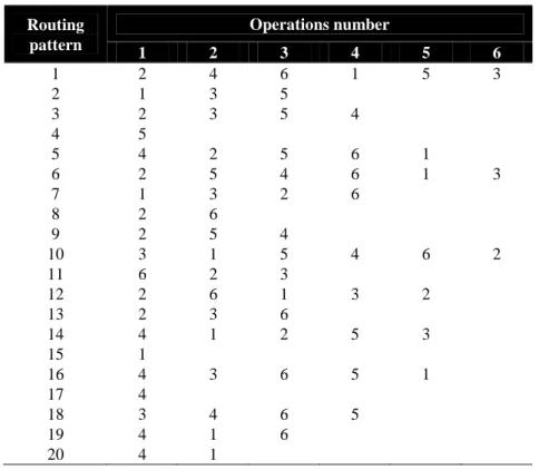
The job shop consists of six workcenters each containing a single multi-purpose machine. In this study, each job routings is randomly chosen from a set of twenty routings each of which with an equal probability of occurrence, see Table 3. The routings were initially randomly generated by defining first the number of operations and afterwards the workcenter for performing each operation, from the first to the last, in the routing. Workcenters were chosen from a discrete distribution ranging from 1 to 6. Return visits to a workcenter are not allowed. As a result of the number of operations in each of the twenty routings the mean number of operations per routing is 3.6. Although most real job shops exhibit a prevalent flow pattern, it is used here a random flow because it represents a more difficult problem (Ragatz and Mabert, 1988).

The time between jobs arrivals follow an exponential distribution. The processing times for all machines are identical, following a 2-Erlang distribution with a mean of 1 time unit. According to Oosterman et al. (2000) the 2-Erlang distribution approaches well the observations made in real life job shops. An average planned system utilization of 90% is created in the shop by setting the appropriate time between arrivals under immediate release. This time between arrivals is then used in the simulation experiments. Immediate release means that no mechanism restricts order release into the system.

Due dates are set externally and modelled as a random variable. They are established using immediate release and ensuring that the number of tardy jobs falls between 5% and 10%. This is achieved using rolling in time uniform distribution of due dates between 50.8 and 60.8 time units (see Table 1). Due dates are assigned to jobs on their arrival to the system. After the assignment of the due date, each job is placed in the pool waiting for release. Job release decisions are made periodically in the beginning of each release period. Each job is considered for release according to the earliest planned release date. Planned release dates are determined by backward scheduling from the due date, using the planned lead times:

j r j j s s S d LT ∈ = −

∑

Where LTs is the planned workcenter lead time and, for each job j, rj is the planned release date, dj is

the due date and Sj is the set of workcenter s in the job routing. Planned work centre lead times were

established through some pilot simulation runs, also using immediate release, under the job arrival pattern adopted in the study.

The OR&MFC mechanism used ensures that a job considered for release is released only if it fits the established workload norms for each workcenter or capacity group. If a job is released, the workload of each workcenter is updated accordingly. Otherwise the job is kept in the pool of jobs to release, until the next release time arrives. The next job in queue is then considered for release. Job releasing decisions are dependent on workcenter s’ workload and on restrictions imposed by workload norm levels adopted for each workcenter. In this work these levels are the same for every workcenter.

Jobs follow a first-in-first-out (FIFO) dispatching rule in all workcenter s. Setup times have been considered sequence independent and assumed as part of the operation processing time.

[Insert Table 3]

3.2 Experimental Design

The following four control factors, i.e. independent variables, were evaluated: the workload accounting over time, the workload control strategy, the release period, and the time limit. Workload accounting and workload control are order release dimensions (see classification in Bergamaschi et al. 1997). The release period and the time limit are two important parameters of the WLC concept. Past studies have shown that the settings of these parameters can have a great influence on systems performance (see for example Land, 2006).

The release period (RP), which determines the interval between releases, is associated with the discrete time convention. The timing convention strategy determines if decisions for orders release

should be carried out on a continuous basis or at discrete time intervals. In this latter case the release period needs to be defined.

In this work, assuming the discrete time convention, the influence of the release period is studied. This factor is tested at two levels: 8 time units and 4 time units. Reducing the release period may reduce the time a job spends in the pool, and eventually in the system. This means increased system performance. However, the release period reduction is likely to reduce the choice of jobs to release which fit workload norms, due to an expected smaller number of jobs available in the pool, and, therefore, a decrease in system performance may occur. So a good system performance requires fine tuning of the release period which is dependent on both shop and jobs characteristics.

The time limit factor is associated with job release times, rj. If we consider the time limit to be

infinite then, when the release time arrives, all available orders in the pool, independent of their release times, are considered for release. If there is a finite value to the time limit, this means that only the orders having release time falling within the time limit, i.e. orders that are urgent, are considered for release. All others must wait. As an example for this latter case, consider that the planned release time of an order is in the time 811. At the time 800 order release are due to take place, if the time limit is 16 (twice the release period of 8 time units), then the order will be considered for release. However, if time limit is 10 time units, then the order only will be

considered for release in the next period, i.e. at time 808. Actually, all other jobs with release times between 808 and 818 will be considered for releasing. Time limit should always be at least as large as the release period to avoid the delay of order in the pool.

The time limit was tested at two levels: infinite time limit and a time limit twice the RP. The workload accounting over time dimension, defines the method of accounting the load of a released job, establishing when and how much of this load should be allocated to each workcenter. The workload accounting is tested at two levels: atemporal and probabilistic. Under the atemporal approach the released job is assumed to instantaneously add up load to each workcenter or capacity group on the basis of the job processing time. This study uses the adjusted aggregated load method

introduced by Oosterman et al. (2000). More specifically, it is assumed that a job j contributes pji/oji

for the aggregated load of a particular workcenter i. Where, pji, is the processing time of job j at

workcenter i and oji represents the position of the workcenter i in the job routing.

The probabilistic approach uses the conversion technique developed by Bechte (1988), to calculate the workload contribution for each workcenter, at each time jobs’ release takes place, based on jobs loaded. The technique is also explained by Breithaupt et al. (2002).

The workload control dimension, influences job release decisions with basis on the strategy adopted. Release decisions are normally based on four workload control strategies, namely upper bound, lower bound, upper and lower bound and workload balancing. In this study the workload control factor is tested at three levels: the upper, the lower and the balancing strategies. In the first strategy, the release of a job to the shop floor is allowed only if workload in all of the workcenter s of a job routing is below the upper bound norm. This means that a job will not be released if, as a result of releasing, at least in one workcenter in the job routing the workload becomes larger than the upper bound. In the second strategy, the release seeks to avoid ‘starving’ of workcenter s by ensuring that workload in all the workcenter s is above the lower bound norm. This means that a job will be released if at least in one workcenter in the job routing, the workload is lower than the lower bound norm. In the third, workload control is achieved by workload balancing. Releases are made only if the job contributes to a better load balancing between workcenter s. However, we restrict the workload on the shop by ensuring that the upper bound load limit of each workcenter in the job’s routing is not exceeded in more than 20%. This value was established after some pilot simulation runs, and leads to good results in this study. The workload balancing measure employed was one of the balance index (BI) used by Garetti et al. (1990), i.e.:

{ }

∑

where Fij represents the workload on workcenter i resulting from the releasing of job j into the shop

floor, and m the number of work centres. The best balancing situation is obtained for BI equals to one.

3.3 Performance Measures

Five measures of the shop performance were collected. These measures are of two types: job and shop oriented measures.

(1) Job oriented measures encompasses the mean tardiness, the percentage of tardy jobs and the standard deviation of job lateness. These statistics have been studied extensively in the literature and evaluate the shop’s ability to meet due dates.

(2) Shop oriented measures encompasses the mean shop flow time and the mean time in system, i.e. the time a job spends waiting in the pre-shop pool plus shop flow time.

4. Analysis and Discussion of Results 4.1 Main experiments

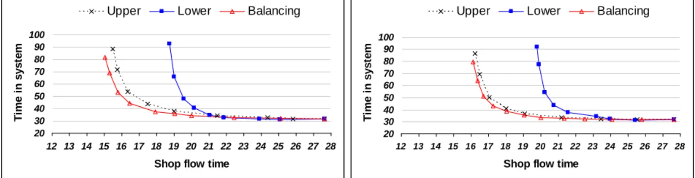
This section presents and discusses the results of the simulation study described above. Figure 1 show the time in system behaviour for each one of the workload control strategies considered under the atemporal and the probabilistic workload accounting over time approaches. In this figure the average value of the time in system is plotted against the shop flow time. Superior mechanisms or strategies yield a lower time in system for a given shop flow time, i.e. will have a curve which is lower and shifted to the left. A point on the curve is the result of simulating the strategies at a specific norm level. Norms of two strategies are equally tight, if they result in the same shop flow time (Oosterman et al., 2000).

As can be seen the curves converge at the highest value of the shop flow time. This is the result of an infinite workload norm level, i.e upper and lower bounds are both very large. As could be expect all strategies give the same results if release is not restricted by workload norms. However, as

norms get tighter, i.e. as shop flow time decreases, time in system increases. In fact, the waiting time on the shop floor is substituted by waiting time in the pool of orders. Below a critical point the performance deteriorates, i.e. time in system increases substantially without any meaningful

reduction of shop flow time. This point is around a shop flow time of 19 time units for the upper and the balancing workload control strategies. The lower bound strategy reaches its critical point sooner, i.e. for a higher value of shop flow time, than the other strategies. This holds for both, atemporal and probabilistic approaches. Workload balancing shows the best performance, i.e. it reaches the critical point latest and it shows identical or lower values of time in system at each level of norm tightness.

[Insert Figure 1]

Tables 4 shows the simulation results for the performance measures described in Section 3.3. This table provides information about the workload accounting over time and workload control strategies, when it is used a release period of 8 time units. Comparisons among the order release dimensions levels have been developed by collecting simulation data at the same point in the time in system vs. shop flow time curve, i.e. at the same shop flow time. Simulation data were collected at a shop flow time of 19 time units, near the critical point for the upper and balancing strategies. This represents a 39.9% reduction of the average shop flow time relatively to an infinite norm level. The atemporal approach, with a lower bound strategy, is not represented in the table because no values for that shop flow time can be obtained from the simulation, as figure 1 clearly shows.

[Insert Table 4] The analysis of results leads to three major conclusions.

First, workload balancing is the best workload control strategy for both, probabilistic and atemporal workload accounting strategies. Significant differences in the performance results are identified on the basis of paired t-tests with 95% confidence level. For each performance variable analysed, the Kolmorov Smirnov test to Normality was carried out, and no statistical evidence was detected for rejecting the null hypothesis at 95% confidence level (p value < 0.05).

The workload balancing performs better than the upper bound strategy for all the performance measures studied. For example it reduces the percentage of tardy jobs in 15.5% for the atemporal approach and in 20.6% for the probabilistic one.

Second, the atemporal workload accounting performs better than the probabilistic one, for all the performance measures studied, under the balancing and the upper bound strategies. For the lower bound strategy, we see superior results under the probabilistic approach. Differences are significant at 95% confidence level. The study here undertaken indicates that the behaviour of the workload accounting dimension may vary according to workload control strategies. A previous study on this mater by Cigolini et al. (1998) observed that the performance of the atemporal strategy is almost as good as the probabilistic one. This study does not use the adjusted aggregated load method within the atemporal strategy of the workload accounting dimension, as we do in our study. Another study developed by Oosterman et al. (2000), conclude that the LOOR mechanism, which uses

probabilistic workload accounting over time, performs better than the ALW mechanism, which uses the atemporal strategy, when the adjusted aggregated load method. These studies compare full WLC mechanisms and not single order release dimensions of them as it is done in this work. Third, it seems that the lower bound workload control strategy do not allow as good control as the other strategies.

We have seen in section 3.2, on one hand that, under the upper bound strategy, a job will not be released if, as a result, at least in one workcenter in the job routing the accounted workload becomes larger than the upper bound norm and that, on the other hand, under the lower bound strategy, a job will be released if, at least in one workcenter in the job’s routing the accounted workload is lower than the lower bound norm. Due to this, we can expect that for the same load or WIP in the shop floor, in which the lower bound in all workcenter s is below workcenter s accounted load level, as exemplified in Figure 2, no jobs will be released into the shop when the lower bound strategy is used. However, this may not be the case when the upper bound strategy is used. In fact, the accounted workload in all workcenter s of a job being considered for releasing may be smaller then

the upper bound norm and therefore, the job would be released. This, in the opinion of the authors, is the reason why the shop in system is lower for the same shop flow time under the upper bound strategy than under the lower bound one.

The performance of the balancing strategy can be explained by identical reasons, because it is based on the upper bound strategy allowing the load limit to go 20% above the upper norm level whenever balancing index can be improved by job release.

[Insert Figure 2]

Figure 3 shows the behaviour of the workload control strategy for two release periods, namely 8 and 4 time units, and the two workload accounting approaches, namely atemporal and probabilistic. The three workload control strategies show better results with an order release period of 4 time units. Moreover, an important conclusion is that the probabilistic approach seems to be more robust to adjustments in the release period length, particularly when combined with the balancing

workload accounting strategy. In fact, when changing the release period, the probabilistic approach leads to a minor variation on the time in system measure.

[Insert Figure 3]

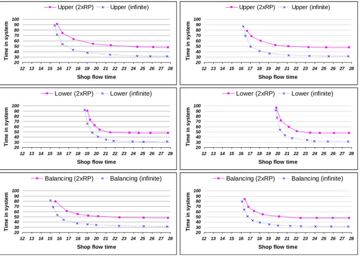
Figure 4 shows the time in system for the workload control and workload accounting strategies under the influence of the time limit factor. For all strategies, results are worse with a finite time limit than under an infinite one. The finite time limit is twice the release period (2xRP), i.e. 16 time units. The use of a finite time limit restricts the release of jobs to those that are urgent, reducing the opportunities to select jobs for release that fit the workload norms, and, therefore, increases time in system of jobs. This result was somehow expected and is in accordance with results of previous works. Land (2006) for example, considers that the use of a finite time limit should only be considered under specific circumstances.

4.2 Robustness Analysis

The second phase of this work involves a robustness analysis of the factors previously studied to changes in three environmental factors, namely the processing time variability, the planned system utilization and variability in time between arrivals of orders to the pool.

Table 5 gives an overall view of the factors studied and the assignment of the corresponding levels. [Insert Table 5]

Operations processing time variability is a source of perturbation and can have an effect on system performance. In balanced flow lines, for example, tend to highly decrease systems utilization. Variability of processing times can be due to several reasons. First due to the natural influence of human work on processing times of operations and second, to a variety of perturbations that can occur in the shop floor, namely, unavailability of the required machines, and variations in lot sizes, materials supply and set-ups, to mention only a few.

To represent the high variability in processing times an exponential distribution is used, and to represent a more stable situation the 2-Erlang distribution, mentioned in section 3.1, is considered. The mean processing time is the same for both distributions and equal to 1 time unit.

The average planned system utilization can be measured as a percentage of the overall shop

capacity used and is dependent on the amount of work released by the planning system into the pre-shop pool or orders release pool. According to Cigolini et al. (1998) this utilization has an important effect on the systems performance. In our study the utilization factor is tested at two levels: 90% and 80%.

The planning system may or may not control the jobs arrivals to the pool. The former is based on smoothed schedules, while the latter is indicative of a non effective planning system, i.e. no

smoothing is carried out. These two types of jobs arrival are simulated in this study. Controlled job arrivals are simulated using constant time intervals between successive arrivals, while uncontrolled job arrivals are simulated using exponential distributed time intervals. In both situations an identical mean is used.

Because this experimental setup requires additional runs of the simulation model, this analysis was carried out only for a subset of the control factors and levels from the main experiments which were considered of special relevance, namely that work well. Table 6 shows the control factors studied and the assignment of the corresponding levels. Besides the influence of the control factors the influences of their interactions were studied as well.

[Insert Table 6]

The approach used to plan the experiments is based on the Taguchi method. The method explicitly models the effects of environmental variations on the four order release factors, and thus provides guidance for implementing OR&MFC mechanisms in uncertain environments. The experimental design employed an inner L16(215) orthogonal array for control factors and an outer L4(23)

orthogonal array for environmental (noise) factors. The inner array has 16 rows, corresponding to the number of trials, with 15 columns at two levels. Factors and interactions are assigned to the columns. The outer array has 3 rows, corresponding to different kinds of industrial environments, where OR&MFC mechanisms should operate. A trial number specifies a test condition with respect to control factors, but the outer array specifies four test conditions with respect to the noise factors to that trial. This means that the experimental design is made of 64 separate tests, and an identical number of simulations runs is needed.

One of the key features of the Taguchi method is the use of a robustness measure called signal-to-noise (S/N) ratio. The S/N ratio aggregates information on the average performance and its variability. The S/N ratio the smaller-the-better characteristic is as follows (Ross, 1988):

2 1 1 / 10 log n ij i S N y n ₌   = −   

∑

where yij is the individual response value from the ith combination of control factors, and jth

combination of noise factors and n the total number of combinations of noise factors for each combination of control factors. Since the performance measure under study is the time in system, the smaller-the-better S/N ratio is used.

All test conditions with respect to control factors have been developed by collecting data at shop flow time of 19 time units, which we consider to be near the critical point for the curves of the time in system versus shop flow time used in this study. By applying equation 3, the S/N ratio values for each level of the control factors can be calculated. The S/N ratio is treated as a response of the experiment and is a measure of the variation within a trial when noise factors are present. Table 7 summarises the results of the tests. According to the Taguchi method, the best level for each factor, that is, the level with the lowest variation across the combination of noise factors is the level with the highest S/R ratio value (Ross, 1988).

[Insert Table 7]

Results show that the atemporal workload accounting and the balancing workload control strategies seem to be the most robust approaches to the influence of the environmental perturbations, due to processing time variability, planned system utilization and variability in time between arrivals of orders to the pool.

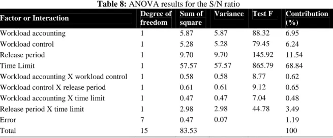
The statistical analysis was performed using analysis of variance (ANOVA). Table 8 shows the results of the ANOVA using the S/N ratio as response. This analysis was undertaken for the level of significance of 5%, i.e. for a 95% confidence level. The last column of the table indicates the

percent contribution (p) of each factor on the total variation, indicating then the degree of influence on the system performance. A small variation in a factor with high percent contribution will have a great influence on the overall systems performance. According to table 8 data, the time limit and the release period are the major factors affecting the system performance, with p=68.84% and

p=11.54%, respectively. The percent contribution of the OR&MFC workload accounting dimension is 6.95% and from workload control dimension is 6.24%. Interactions do not present contribution percentages of significance on the system performance, since these are smaller than the

experimental error of 1.19%. An exception is the interaction between the timing convention and the time limit, which is 3.49%. Part of this interaction may be due to the experimental setting, in

particular due the fact that, one of the levels of time limit was set in the experimentation as a function of the release period, i.e. 2xRP.

[Insert Table 8]

Some important findings can be obtained from the results. We can clearly see that the time limit is really the factor with the highest contribution for variability. This indicates that it is a strong perturbation factor and, as already found in the main experiments section, highly influential of systems performance. Therefore, care must be taken in establishing its level in order to ensure that good performance is achieved.

In reviewing the results the following issues deserve special attention for the selection and implementation of an OR&MFC mechanism in practice:

1) The release period and in particular the time limit parameters are much more sensitive to productive environmental perturbations and highly influential of system performance than are the strategies associated with the workload control and workload accounting dimensions.

2) The choice of time limit and release period levels are of special importance because they influence in a strong manner the performance behaviour of the OR&MFC mechanisms. 3) Although no interaction has been identified among the factors considered in the robustness analysis, which means that the effect of a factor does not depends on the level of the other, the experiences carried out in section 4.1 show that there are some recommendations to put forward related with strategies of workload control and workload accounting dimensions. Thus, if the lower bound workload control strategy is adopted the workload accounting strategy must be one, i.e. the probabilistic strategy; however, if the upper bound or balancing strategy are used instead, than the workload accounting must be another, i.e. the atemporal strategy. Moreover, workload control balancing strategy, for the productive environment studied, is the most robust to environmental factors variability. Therefore better results can be expected from it, when implemented in practice, than from the other two strategies tested. Additionally, the atemporal workload accounting strategy,

for the productive environment studied, is the one which works best, i.e. is the most robust to environmental factors, and, therefore, better results may be obtained from its application in practice.

5. Conclusions and further work

Order release and materials flow control (OR&MFC) mechanisms are strategically important for the economic success of companies because they have a great influence on company operations

performance. However, the behaviour and performance of these mechanisms highly depend on the OR&MFC operating parameters settings related with order release dimensions and with the

production control, including the nature of the environmental factors such as system utilization and variability of processing times and in time between arrivals of jobs to the shop floor.

In this work the effectiveness and influence of order release strategies, in a job shop environment was assessed by studying dimensions and parameters of order release mechanisms. Two dimensions were particularly investigated: the workload accounting over time and the workload control

strategy. The parameters evaluated were the time limit, related with the timing convention, and also the release period.

Two important conclusions resulted from the study. First, workload balancing performs better than the other workload control strategies tested, namely the upper bound and the lower bound ones. Second, the atemporal workload accounting over time strategy works better and is more robust than the probabilistic strategy, to variation in the system environmental factors. However we notice that the probabilistic strategy seems to be more robust to variation in the release period.

This research work can be seen as an important contribution for the better understanding of the behaviour of order release and materials flow control mechanisms. From the study directions were pointed out for setting OR&MFC dimensions and parameters for good production systems

operation. However, due to the enormous variety of strategies and control parameters that influence systems performance, it is recognised the need to further work on the matter for better

production environments. As an example, in relation to the study here carried out, due to the impact and good behaviour of the balancing strategy, it is worth testing it at upper allowance limits

different from the 20% considered.

References

Bechte, W., 1988, Theory and practice of load-oriented manufacturing control, International Journal of Production Research, 26(3), 375-395.

Bergamaschi, D., Cigolini, R., Perona, M. and Porioli, A., 1997, Order review and release strategies in a job shop environment: a review and classification, International Journal of Production Research 35 (2), 339-420.

Breithaupt, J.W., Land, J. and Nyhuis, P., 2002, The workload control concept: theory and practical extensions of Load Oriented Order Release, Production Planning and Control, 13(7), 625-638. Cigolini, R. and Portioli, A., 2002, An experimental investigation on workload limiting methods within ORR policies in a job shop environment, International Journal of Production Research, 13(7), 602-613.

Cigolini, R., Perona, M. and Portioli, A., 1998, Comparison of order review and release techniques in a dynamic and uncertain job shop environment, International Journal of Production Research, 36(11), 2931-2951.

Fernandes, N.O. and S. C. Silva, 2005, A generic workload control model for order release and workflow control, 18th International Conference on Production Research, Fisciano - Italy.

Fowler, J.W., Hogg, G.L. and Mason, S.J., 2002, Workload control in the semiconductor industry, Production Planning and Control, 13(7), 568-578.

Garetti, M., Pozzetti, A. and Bareggi, A., 1990, On-line loading and dispatching in flexible manufacturing systems, International Journal of Production Research, 28(7), 1271-1292. Graves, R.J., Konopka, J.M. and Milne, R.J., 1995, Literature review of materials flow control mechanisms, Production Planning and Control 6 (5), 395-403.

Haskose, A., Kingsman, B.G. and Worthington, D., 2004, Performance analysis of make-to-order manufacturing systems under different workload control regimes, International Journal of

Production Economics, 90 (2), 169-186.

Hendry, L. and Kingsman, B.G., 1991, A decision support system for job release in make-to-order companies, International Journal of Operations and Production Management, 11, 6-16.

Henrich, P., Land, M. and Gaalman, G.J.C., 2004, Exploring applicability of the workload control concept, International Journal of Production Economics, 90 (2), 187-198.

Kingsman, B.G., 2000, Modeling input-output workload control for dynamic capacity planning in production planning systems, International Journal of Production Economics, 13 (7), 73-93.

Land, M., 2006, Parameters and sensitivity in workload control, International Journal of Production Economics, (in Press).

Little, J.D.C., 1961, A proof for the queuing formula: L=λW, Operations Research, 9, 383-387. Melnyk, S.A. and Ragatz, G.L., 1989, Order review/release: research issues and perspectives, International Journal of Production Research, 27 (7), 1081-1096.

Melnyk, S.A., Tan, K.C., Denzler, D.R. and Fredendall, L., 1994, Evaluating variance control, order review/release and dispatching: a regression analysis, International Journal of Production Research, 32 (5), 1045-1061.

Oosterman, B., Land, M., Gaalman, G.J.C., 2000, The influence of shop characheritics on workload control, International Journal of Production Economics, 68, 107-119.

Ragatz, G.L., Mabert, V.A., 1988, An evaluation of order release mechanism in job shop environment, Decision Sciences, 19, 167-189.

Ramasesh, R., 1990, Dynamic Job shop scheduling: a survey of simulation research, Omega, 18 (1), 43-57.

Ross, P.J., 1988, Taguchi Techniques for Quality Engineering: Loss Function, Orthogonal Experiments, Parameter and Tolerance Design, McGraw-Hill, New York.

Stevenson M. and Hendry L., 2006, Agregated Load-oriented workload control: A review and re-classification of a key aproach, International Journal of Production Economics, In Press.

Tayur, S.R., 1993, Structural properties and a heuristic for kanban-controlled serial lines, Management Science 39 (11) 1347-1368.

Wight, O.W., 1970, Input/output control: a real handle on lead time, Production and inventory Management Journal, 11(3), 9-31.

Table 1: shop floor operation conditions

Characteristic Value

Shop type Job shop

Workcenter s Six with one machine each

Operations per job Discrete(1,6)

Setup times Sequence independent

Due date allowance Uniform (50.8,60.8)

Processing times 2-Erlang (1)

Table 2: Production control conditions

Characteristic Value

Workload norms Stepwise down from infinite

Dispatching rule FIFO

Planned system utilization 90%

Table 3: workcenter job routing matrix Routing pattern Operations number 1 2 3 4 5 6 1 2 4 6 1 5 3 2 1 3 5 3 2 3 5 4 4 5 5 4 2 5 6 1 6 2 5 4 6 1 3 7 1 3 2 6 8 2 6 9 2 5 4 10 3 1 5 4 6 2 11 6 2 3 12 2 6 1 3 2 13 2 3 6 14 4 1 2 5 3 15 1 16 4 3 6 5 1 17 4 18 3 4 6 5 19 4 1 6 20 4 1

Table 4: Overall performance results

* Best Values

Table 5: Noise factors

Factor Level 1 Level 2

Planned system utilization 90% 80%

Processing time variability 2-Erlang Exponential

Variability in time between arrivals Exponential Constant

Table 6: Control factors

Factor Level 1 Level 2

Workload accounting over time Atemporal Probabilistic

Workload control Upper bound Balancing

Release period 8 time units 4 time units

Time limit infinite 2 times the release period

Table 7: S/N ratio values (dB)

Factor Level 1 Level 2

Workload accounting over time -32,45* -33,66

Workload control -33,63 -32,48*

Release period - discrete -33,83 -32,27*

Time limit -31,15* -34,95

* Best level

Performance measures

Probabilistic Atemporal

lower upper balancing upper balancing

Shop flow time 19.0119±4.60 19,0135±0.08 19.0275±0.12 19.0720±0.10 19.0273±0.12

Time in system 65.6414±0.13 37.9794±0.93 35.5487±0.65 36.6219±0.80 35.1029±0.60*

Percent Tardy jobs 46.4698±3.37 18.4869±1.05 14.6694±0.69 16.3615±1.13 13.8308±0.80*

Tardiness 20.6206±3.67 3.5526±0.56 2.7111±0.27 2.4358±0.36 2.1802±0.24*

Table 8: ANOVA results for the S/N ratio Factor or Interaction Degree of

freedom

Sum of square

Variance Test F Contribution (%)

Workload accounting 1 5.87 5.87 88.32 6.95

Workload control 1 5.28 5.28 79.45 6.24

Release period 1 9.70 9.70 145.92 11.54

Time Limit 1 57.57 57.57 865.79 68.84

Workload accounting X workload control 1 0.58 0.58 8.77 0.62

Workload control X release period 1 0.61 0.61 9.12 0.65

Workload accounting X time limit 1 0.47 0.47 7.04 0.48

Release period X time limit 1 2.98 2.98 44.78 3.49

Error 7 0.47 0.07 1.19

20 30 40 50 60 70 80 90 100 12 13 14 15 16 17 18 19 20 21 22 23 24 25 26 27 28

Shop flow time

T im e i n s y s te m

Upper Lower Balancing

20 30 40 50 60 70 80 90 100 12 13 14 15 16 17 18 19 20 21 22 23 24 25 26 27 28

Shop flow time

T im e i n s y s te m

Upper Lower Balancing

Probabilistic Atemporal

Figure 1: time in system behaviour

w1 w2 w3 w4 w5 w6

Load

(hours) Upper bound

Lower bound

Workcenters

20 30 40 50 60 70 80 90 100 12 13 14 15 16 17 18 19 20 21 22 23 24 25 26 27 28

Shop flow time

T im e i n s y s te m

Balancing (4 time units) Balancing (8 time units)

20 30 40 50 60 70 80 90 100 12 13 14 15 16 17 18 19 20 21 22 23 24 25 26 27 28

Shop flow time

T im e i n s y s te m

Lower (4 time units) Lower (8 time units)

20 30 40 50 60 70 80 90 100 12 13 14 15 16 17 18 19 20 21 22 23 24 25 26 27 28

Shop flow time

T im e i n s y s te m

Upper (4 time units) Upper (8 time units)

20 30 40 50 60 70 80 90 100 12 13 14 15 16 17 18 19 20 21 22 23 24 25 26 27 28

Shop flow time

T im e i n s y s te m

Lower (4 time units) Lower (8 time units)

20 30 40 50 60 70 80 90 100 12 13 14 15 16 17 18 19 20 21 22 23 24 25 26 27 28

Shop flow time

T im e i n s y s te m

Upper (4 time units) Upper (8 time units)

20 30 40 50 60 70 80 90 100 12 13 14 15 16 17 18 19 20 21 22 23 24 25 26 27 28

Shop flow time

T im e i n s y s te m

Balancing (4 time units) Balancing (8 time units)

Probabilistic Atemporal

20 30 40 50 60 70 80 90 100 12 13 14 15 16 17 18 19 20 21 22 23 24 25 26 27 28

Shop flow time

T im e i n s y s te m

Upper (2xRP) Upper (infinite)

20 30 40 50 60 70 80 90 100 12 13 14 15 16 17 18 19 20 21 22 23 24 25 26 27 28

Shop flow time

T im e i n s y s te m

Lower (2xRP) Lower (infinite)

20 30 40 50 60 70 80 90 100 12 13 14 15 16 17 18 19 20 21 22 23 24 25 26 27 28

Shop flow time

T im e i n s y s te m

Balancing (2xRP) Balancing (infinite)

20 30 40 50 60 70 80 90 100 12 13 14 15 16 17 18 19 20 21 22 23 24 25 26 27 28

Shop flow time

T im e i n s y s te m

Lower (2xRP) Lower (infinite)

20 30 40 50 60 70 80 90 100 12 13 14 15 16 17 18 19 20 21 22 23 24 25 26 27 28

Shop flow time

T im e i n s y s te m

Upper (2xRP) Upper (infinite)

20 30 40 50 60 70 80 90 100 12 13 14 15 16 17 18 19 20 21 22 23 24 25 26 27 28

Shop flow time

T im e i n s y s te m

Balancing (2xRP) Balancing (infinite)

Probabilistic Atemporal