Mapping reference crop evapotranspiration in Bahia, Brazil, using Hargreaves-Samani method | Mapeando a evapotranspiração de culturas de referência na Bahia, no Brasil, usando o método Hargreaves-Samani

(1)

Received: March 24, 2016 | Approved: August 06, 2016.

GEAMA Journal

The Journal of environment

Scientific Article

Mapping reference crop evapotranspiration in Bahia, Brazil, using

Hargreaves-Samani method

Neilon Duarte da Silva B.Sc.

a

_{.*, Aureo Silva de Oliveira Ph.D.}

b

_{, Tatyana Keyty Souza}

Borges M.Sc.

a

_{Ludmila Ferreira Gomes St.}

a

_{, Sandy Sousa Fonseca St.}

a

_{, Fabineia Amaral}

Guedes St.

a

_{, João Paulo Chaves Couto B.Sc.}

a

_.

a_{Centro de Ciências Agrárias Ambientais e Biológicas, Universidade Federal do Recôncavo da Bahia, Brasil.} b_{Professor Associado,}_{Centro de Ciências Agrárias Ambientais e Biológicas, Universidade Federal do Recôncavo da}

Bahia, Brasil.

__________________________________________________ *Corresponding author: E-mail: neylon_duart@hotmail.com

ABSTRACT

The objective of this work was to study the spatial behavior of the reference evapotranspiration (ETo) in the state of Bahia according to the method of 1985

Hargreaves Samani. The study includes data from 452 meteorological weather stations managed by the National Institute of Meteorology (INMET) and the National Water Agency (ANA). These stations have data of maximum, minimum and average temperatures covering the period from 1965 to 2013. Monthly maps of spatial distribution of ETo were made by geostatistical techniques with ArcGIS 9.3 software.

There is also predominance of higher evaporative demands in the north of the state. The month with the highest spatial dependence of ETo was the month of October, with

similar results were observed for the months of May, July, August and September. The values of spatial dependence obtained in these respective months showed an average range of 1.07 degrees. The ETo rates corresponding to the Atlantic Forest areas near the

Atlantic coast in the east are uniformly distributed where predominate Humid and Super-Moist climates. Alternative models to combination equations such as Penman-Monteith provide easier and reliable way to carry out studies on ETo estimation for

water resources management. The geostatistical methods are important tools for regionalizing meteorological variables, including ETo.

Keywords: Meteorology, GIS, geostatistic, evapotranspiration

INTRODUCTION

Evapotranspiration (ET) is one of the primary variables for most of hydrological processes in nature and its knowledge is crucial at any spatial scale for

water resources management. Rates of ET at drainage basin levelare essentially determined by type of vegetation, soil moisture availability and meteorological conditions (SUN et al., 2004).

(2)

In the context of water use in agriculture, the concept of a reference crop ET (ETo) is related to the

net water demand by other crops (ETc) through a

conversion factor called crop coefficient (Kc), which

can generally vary from 0,1 to 1,3 according to crop type, frequency of wetting events (irrigation or rain) and crop development stage (SILVA et al, 2015; ROCHA et al, 2016).On the other hand, because ETo

essentially depends on atmospheric parameters, its concept is useful as an indicator of the general type of climate in a regionfrom humid (low ETo) to arid

(high ETo) climate (ALLEN et al., 1998).

Reference ET rates can be determined by different methods generally classified into direct (measurement) and indirect (estimation) ones. Lysimeters measure ETo while mathematical models

based on atmospheric variables are used to estimate it. The Penman-Monteith equation modified by the UN-FAO, known as FAO-56 Penman-Monteith equation (FAO-56 PM) (ALLEN et al., 1998), is considered a standard in providing quality estimations of ETo across different climates.

The FAO-56 PM method and other formulations of the so-called combination equations, require large amounts of reliable data on incident solar radiation, wind speed, air temperature, and relative humidity. Such demand for complete series of data imposes restrictions when one desires to generate maps of ETo for large areas due to the lack of enough

information at the desired density. In such cases, equations based on fewer atmospheric parameters

like the 1985-Hargreaves-Samani equation

(HARGREAVES& SAMANI, 1985; HARGREAVES & ALLEN, 2003), which requires only air temperature as input variable, can be an alternative to the more data-demanding methods.

Geographic Information Systems (GIS) are powerful tools that allow spatial analysis of large sets of climatological data. In association to geostatistical techniques, GIS has presented interesting results in studies related to spatial

variability, mapping and quantization of

meteorological phenomena on monthly and annual basis (HASHMI et al., 1995; VIEIRA, 1997; SOUZA et al., 1998).

The usage of regionalized information on climate variables finds special applications in the field of water resources management. In this context, geostatistical techniques, particularly methods of interpolation such as Kriging have been applied with success on spatialization of meteorological variables, with superior results when compared to alternatives like inverse distance weighting, spline interpolation or natural neighbor (MELLO et al. 2003; ALVES et

al. 2008; SILVA et al. 2010; GARDIMAN JUNIOR

et al. 2012).

Many studies (BARBOSA et al., 2005, BELTRAME et al., 1994; CHUNG et al., 1997) have reported maps of reference ET from GIS techniques for many parts of the world. They concluded that their methodologies allowed them to acquire individual ETo values and, therefore, to make more

accurate water demands evaluations in the region. This paper aimed at analyzing the spatial distribution of reference ET in the state of Bahia by means of GIS and geostatistical techniques from historical series of weather data with the hope that such results can be useful for farmers at local level as well as for planners and decision makers at the government level.

(3)

MATERIALS AND METHODS

Region of interest

Due to the large natural variability and complexity of the Bahia territory, it is common to classify its sub regions according to a set of different criteria such as major natural biomes, drainage basins and hydrogeological domains. The state area can then be divided into four major natural biomes: tropical savannah, semi-arid, mountain ranges and Atlantic forest. There are also thirteen major drainage basins: São Francisco (42% of the Bahia territory), Vaza-Barris, Real, Itapicuru, Inhambupe, Recôncavo Norte, Paraguassu, RecôncavoSul,

Contas, Leste, Pardo, Jequitinhonha

andExtremoSul, and five hydrogeological domains: DetritalCoverings, Sedimentary basin, Limestones, Metasediments, Crystalline fissure (SEI, 2012).

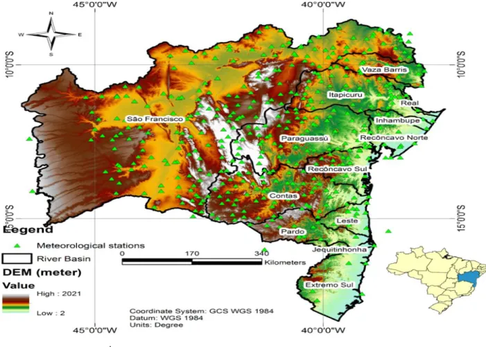
Meteorological data his study is based on monthly averages of meteorological data collected at weather stations of the Brazilian National Institute of Meteorology (INMET) and the Brazilian National Water Agency (ANA) networks. There are altogether 452 meteorological stations in Bahia providing records for maximum, minimum and average temperature. The records used in this work range from 1965 to 2013 with an average of 45 years per station and

Figure 1. Distribution of the weather stations on a digital elevation model of the state of Bahia, showing the limits of the major river basins

.

(4)

Received: March 24, 2016 | Approved: August 06, 2016. Hargreaves-Samani (1985) estimation method

The Hargreaves &Samani (1985) model is shown in Equation 1.



T



Ra

T

ET

o



0 ,

0023



(

m



17 ,

18 )



x



n



₍₁₎ where, ETo– reference evapotranspiration (mmd-1);

Tm – mean air temperature (°C);

Tx– maximumair temperature (°C);

Tn – minimum air temperature (°C);

Ra – extraterrestrial solar radiation (mmd-1). Geostatistical tools

A series of maps was initially built using the Geostatistical Analyst tool in the ArcGIS 9.3 software. Ordinary Kriging was used as interpolation method. Its general formula is presented on Equation 2: vi n i i v

Z





1 '



(2) where,

Z’v – the ordinary kriging estimator for a point v;

λi – ith weight;

Zvi – value of the ith observation for the

regionalized variable, collected on point xi;

n – number of weights.

According to LANDIM (2003), a semivariogram is an important tool for determining weights for spatial continuity and represents a quantitative variation of the regionalized spatial phenomenon. It allows

determining and analyzing the dependency between spatialized points (JOURNEL & HUIJBREGTS, 1978). A semivariogram for kriging regressions is presented on Equation 3:





2 1

)

(

)

(

.

)

(

2

1 )

(











n i i i

Z

x

h

x

Z

h

N

h

y

(3) where, y(h) – estimation;

Z(x) – position of the elements; N(h) – observation pairs; h – distance.

After adjusting the semivariograms the Nugget Effect (Co), sill (Co+C1) and range (Ao) parameters were calculated. When the distance h reaches its maximum value the sill parameter, which represents the maximum limit distance of spatial

dependency, is determined (ISAAKS &

SRIVASTAVA 1989).

An evaluation of spatial dependency is relevant once it provides another parameter for map interpretation. Equation 4, as proposed in CAMBARDELLA et al. (1994), was used in this process. The level of spatial dependence (GD) was classified as: strong, when GD < 25%, moderate, when 25%<75%, and weak, when GD > 75%.

100 C C C GD 1 0 0         

(4) where, GD – dependence level; C0 – nugget effect; (C0 + C1) – sill.

(5)

Received: March 24, 2016 | Approved: August 06, 2016. Model performance

The performance of models and methods for ETo is evaluated using Root Mean Square Error (RMSE) (Equation 5), which is considered an efficient statistical indicator for calibration and evaluation (GAVILÁN et al., 2006; LOPEZ-URREA et al., 2006, JABLOUN & SAHLI, 2008, KUMAR et al., 2002; and AHMADI & FOOLADMAND, 2008) and the Mean Bias Error (MBE) is calculated in Equation 6. The precision of the kriging interpolation on a monthly basis was quantified using the Pearson’s correlation coefficient (r) (Equation 7), and the Willmott index of agreement (d) (WILLMOTT, 1982), Equation 8. n ET ET RMSE n i oEi oOi



   1 2 ) ( (5)





n ET ET MBE n i oOi oEi



   1 (6)



          n 1 i 2 oEi oEi n 1 i 2 oOi oOi n 1

i oOi oOi oEi oEi

) ET (ET ) ET (ET ) ET (ET ) ET (ET r

(7)







 







_               



  n i oOi oOi oOi oEi n i oOi oEi ET ET ET ET ET ET d 1 2 1 2 1 (8) where,

r – Pearson’s correlation coefficient; d – Willmott index of agreement;

RMSE – Root Mean Square Error (mm d-1_);

MBE – Mean Bias Error (mm d-1_);

EToEi – estimated(interpolated) ETo (mm d-1);

EToOi – observed(calculated) ETo (mm d-1);

EToEi – mean estimated (interpolated) ETo (mm d-1);

EToOi – mean observed (calculated) ETo (mm d-1).

RESULTS AND DISCUSSION

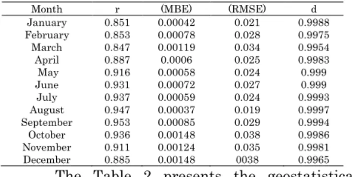
The results of the application of the statistical indicators for mapping ETo over the entire

state of Bahia are shown in Table 1. All models of monthly ETo mapping using kriging interpolation

were satisfactory. A strong positive correlation was verified in all month estimations according to the Pearson’s coefficient. Regarding the MBE and RMSE indicators, for all months these parameters presented positive values tending to zero. This behavior was also observed in several comparisons for different ETo estimation methods by researchers

like AHMADI & FOOLADMAND (2008), LOPEZ-URREA et al. (2006), and GAVILÁN et al. (2006). The Willmott index of agreement (d) was also satisfactory in all months with values around 1, confirming the results reported by LOPEZ-URREA et al. (2006) and SULEIMAN & HOOGENBOOM (2007).

Negative values around -0.225 were found by Vilanova et al. (2012) and Lemos Filho et al. (2007) in studies of ETo spatialization for the state of Minas

Gerais. The values reported in their work for MBE were all near zero, suggesting a super estimation by the model.

Table 1. Statistical indicators for ETo estimation over the state of Bahia

Month r (MBE) (RMSE) d January 0.851 0.00042 0.021 0.9988 February 0.853 0.00078 0.028 0.9975 March 0.847 0.00119 0.034 0.9954 April 0.887 0.0006 0.025 0.9983 May 0.916 0.00058 0.024 0.999 June 0.931 0.00072 0.027 0.999 July 0.937 0.00059 0.024 0.9993 August 0.947 0.00037 0.019 0.9997 September 0.953 0.00085 0.029 0.9994 October 0.936 0.00148 0.038 0.9986 November 0.911 0.00124 0.035 0.9981 December 0.885 0.00148 0038 0.9965

The Table 2 presents the geostatistical parameters of each ETo monthly estimation model

obtained by kriging. In this study, all ETo

spatialization models showed moderate dependence

(6)

level. The spatial variability of meteorological variables may be influenced by different topographic and geographic aspects, specially altitude and proximity to the sea. It may also be affected by other climatic factors such as humidity, wind and vegetation (JIN et al., 2013). Nevertheless, the dominant influence seems to be land topography (BOTH et al, 2010) that affects air temperature in the sense that highest elevations tend to show the lowest values of ETo. Normally the interpolation

methods do not consider the altitude of the sample points, instead, like the kriging method for example, they are based on the distance between the samples and the point of the estimated value, lowering its spatial dependence (BURROUGH, 1986; BETTINI, 2007). According to Table 2, October was the month with the strongest spatial dependence with similar results found for the months of May, July, August and September.

Table 2. Geostatistical parameters of mapping ETo estimated with the Hargreaves and Samani equation

Month C0 C1 C0 + C1 _(degree)Ao GD _% Class January 0.0225 0.0211 0.0436 0.576 51.6 Moderate February 0.0204 0.0231 0.0435 0.818 46.9 Moderate March 0.0183 0.0201 0.0384 0.948 47.7 Moderate April 0.0181 0.0271 0.0452 0.897 40.0 Moderate May 0.0206 0.0404 0.0610 1.021 33.8 Moderate June 0.0187 0.0438 0.0625 0.966 29.9 Moderate July 0.0219 0.0597 0.0816 1.079 26.8 Moderate August 0.0256 0.0612 0.0868 1.099 29.5 Moderate September 0.0244 0.0620 0.0864 1.040 28.2 Moderate October 0.0237 0.0679 0.0916 1.228 25.9 Moderate November 0.0201 0.0346 0.0547 0.865 36.8 Moderate December 0.0191 0.0267 0.0458 0.948 41.7 Moderate

The center part of Bahia, an area called Chapada Diamantina with the highest elevations in the state (Figure 1), is the limit between two major river basins, the São Francisco in the west (the largest) and the Paraguassu river basin in the east. The effect of elevation on air temperature can be appreciated from Figure 2A with the lowest values (18.9 to 22.4o_{C) found in the center-south part of the}

state. On the other hand, Figure 2B shows that the effect of proximity to the Atlantic Ocean is more important on the difference between the maximum and minimum air temperature, with the amplitude increasing from east to west.

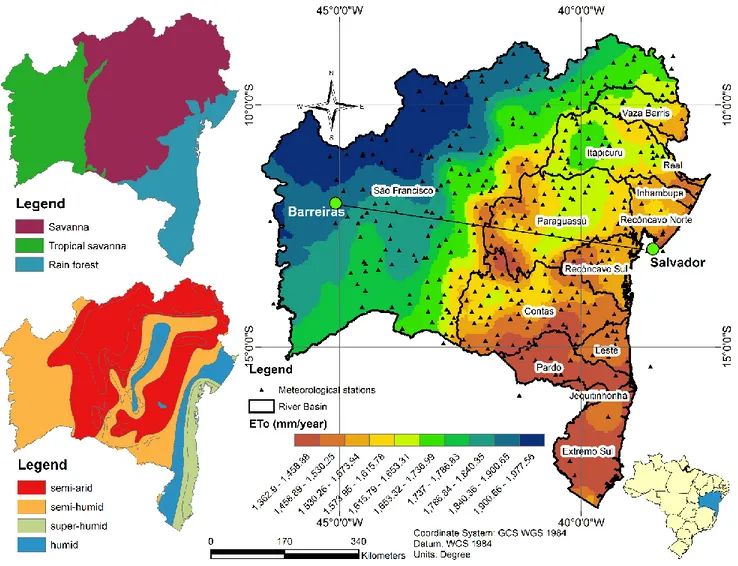
Figure 3 shows the distribution of annual ETo in Bahia. Due to the distribution patterns of

mean air temperature and temperature amplitude, values of ETo based on the Hargreaves-Samani

equation increases from southeast to northwest. The southeast is characterized by humid and super-humid climate. Topographic influences on ETo was

also observed by McVicar et al. (2007) in some regions of China and by Latha et al. (2011) in India.

Figure 2.Distribution of the mean monthly air temperature (A) and the annual temperature amplitude (B) over the Bahia territory

A

B

(7)

Figure 3. Map of ETo values over Bahia in association to vegetation and climate maps

Figure 4 presents the ETo distribution profile given

in Figure 3 between the cities of Barreiras and Salvador, the capital of Bahia. The Tropical Savanna biome, on this profile, presents two types of climate: Semi-Humid and Semi-Arid. There are no considerable variations of ETo on this biome (average

1810 mm), once its topography is very regular. In a study in an arid zone, Jin et al. (2013) found, on a similar ETo profile, the lowest monthly ETo values on

desert and sand zones, while the highest ones on lake territories.

The savannah part of the profile has five sections of climatic typologies. There is also a considerable variation on ETo in this region with values ranging

from 1550 mm to 1770 mm annually. This happens especially due to the effects of altitude over the air temperature, which is a fundamental parameter for the Hargreaves-Samani method of estimating ETo.

(8)

Figure 4. Annual average ETo spatialization profile (SH: Semi-Humid; H: Humid; SpH: Super-Humid; SA: Semi-Arid).

The profile region corresponding to the Atlantic forest presents uniform ETo with Humid

and Super-Humid climates. In general, there is a decrease on ETo values due to the influence of the

ocean.

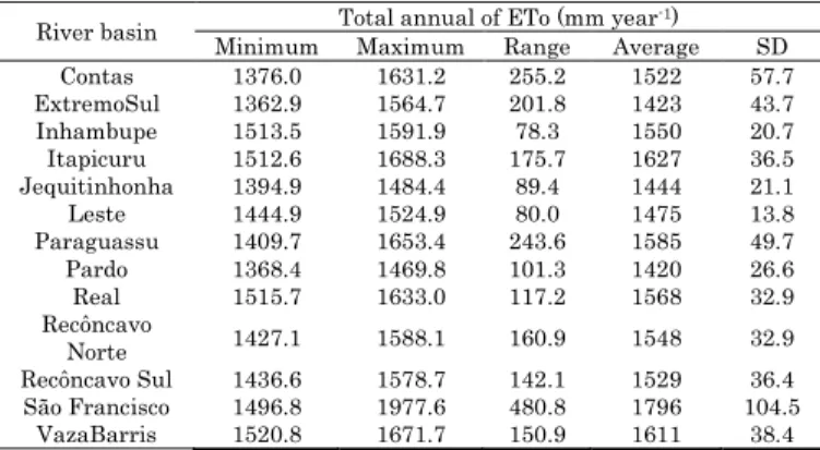
Table 3 presents annual ETo values at

drainage basins level. The São Francisco Basin presents the higher ETo values, also with highest

amplitude. Both the Real and the South Recôncavo drainage basins have similar spatial distribution. The Pardo basin presented the lowest maximum values of ETo during the year. Meanwhile, the Vaza-

Barris basin presented the highest minimum ETo

values annually. The Contas River basin presented the second highest amplitude, followed by the Paraguassu and the Far South basins. The lowest amplitude was observed for the Inhambupe basin.

Table 3. Annual values of ETo for the main drainage basins in Bahia

River basin _Minimum Total annual of ETo (mm year_Maximum _Range _Average-1) _SD Contas 1376.0 1631.2 255.2 1522 57.7 ExtremoSul 1362.9 1564.7 201.8 1423 43.7 Inhambupe 1513.5 1591.9 78.3 1550 20.7 Itapicuru 1512.6 1688.3 175.7 1627 36.5 Jequitinhonha 1394.9 1484.4 89.4 1444 21.1 Leste 1444.9 1524.9 80.0 1475 13.8 Paraguassu 1409.7 1653.4 243.6 1585 49.7 Pardo 1368.4 1469.8 101.3 1420 26.6 Real 1515.7 1633.0 117.2 1568 32.9 Recôncavo Norte 1427.1 1588.1 160.9 1548 32.9 Recôncavo Sul 1436.6 1578.7 142.1 1529 36.4 São Francisco 1496.8 1977.6 480.8 1796 104.5 VazaBarris 1520.8 1671.7 150.9 1611 38.4 SD – Standard derivation CONCLUSIONS

Alternative models to the combination equations for estimating ETo provide easier and

more accessible ways of analyzing

evapotranspiration in a wider range of study fields, with emphasis on management of water resources. Meanwhile, this work confirmed that geostatistical methods are important tools for regionalizing meteorological variables such as ETo.

One important observation was that the ETo

distribution presents spatial dependence in cold months of the year. This kind of analysis allows researchers to amplify their vision and, therefore, Tropical Savannah Savannah Atlantic Forest

(9)

improve management of water resources on a larger scale.

The ETo profiles for the state of Bahia allow

us to observe its distribution continuously, and associate it with corresponding biomes and climatic typologies. It also allows us to analyze its variations regarding other aspects like topography and distance to the sea. Additionally, considering the analysis for each specific drainage basin make it possible to better manage water resources with more efficient decisions.

REFERENCES

AHMADI, S. H., FOOLADMAND, R. H. Spatially distributed monthly reference evapotranspiration derived from the calibration of Thornthwaite equation: a case study, South of Iran. Irrig Sci 26:303–312, 2008.

ALLEN, R. G.; PEREIRA, L. S.; RAES, D.; SMITH,

M Guidelines for computing crop water

requirements. Irrigation and Drainage Paper, 56. Rome: FAO, 1998. 310p.

ALVES, M.; BOTELHO, S. A.; PINTO, L. V. A.; POZZA, E. A.; OLIVEIRA, M. S.; FERREIRA, E.; ANDRADE, H. Variabilidade espacial de variáveis geobiofísicas nas nascentes da bacia hidrográfica do Ribeirão Santa Cruz. Revista Brasileira de Engenharia Agrícola e Ambiental, Campina Grande, v. 12, n. 5, p. 527-535, 2008

BARBOSA, F. C.; TEIXEIRA, A. S.; GONDIM, R. S. Espacialização da evapotranspiração de referência e

precipitação efetiva para estimativa das

necessidades de irrigação na região do Baixo

Jaguaribe–CE. Revista Ciência Agronômica,

Fortaleza, v. 36, n. 1, p. 24-33, 2005.

BETTINI, C. Conceitos básicos de geoestatística. In: MEIRELLES, M. S. P.; CÂMARA, G.; ALMEIDA, C. M. (Ed.). Geomática: modelos e aplicações ambientais. cap.4. Brasília: Embrapa, 2007. BOTH, G. C., HAETINGER, C., JASPER, A., DIEDRICH, V. L., FERREIRA, E. R. Estimativa e espacialização da temperatura dos meses mais quente e frio do estado do Rio Grande do Sul. Caminhos de Geografia Uberlândia v. 11, n. 36 dez/2010.

BURROUGH P. A. Principles of Geographic

Information Systems for Land Resources

Assessment, em "Monographs on Soil and Resources Survey", n. 12, Oxford: Clarendon Press, 1986. CAMBARDELLA, C.A.; MOORMAN, T.B.; NOVAK, J.M.; PARKIN, T.B.; KARLEN, D.L.; TURCO, R.F. & KONOPKA, A.E. Field-scale variability of soil properties in Central Iowa Soils. Soil Sc. Soc. Am. J., 58:1501-1511, 1994.

CHUNG, H. W.; CHOI, J. Y.; BAE, S. J. Calculation

of spatial distribution of potential

evapotranspiration using GIS. In: ASAE ANNUAL INTERNATIONAL MEETING, 1997, Minneapolis, Minnesota. Paper... Minneapolis: American Society of Agricultural Engineers, 1997. 9 p.

GARDIMAN JUNIOR, B. S., MAGALHÃES, I. A. L., FREITAS, C. A. A., CECÍLIO, R. A. Análise de técnicas de interpolação para espacialização da precipitação pluvial na bacia do rio Itapemirim (ES).

(10)

Ambiência Guarapuava (PR) v.8 n.1 p. 61 - 71 Jan./Abr. 2012.

GAVILÁN, P., LORITE, I.J., TORNERO, S.,

BERENGENA, J. Regional calibration of

Hargreaves equation for estimating reference ET in a semiarid environment. Agricultural Water Management 81 257–281, 2006.

HARGREAVES, G.H., SAMANI, Z.A. Reference crop evapotranspiration from temperature. Appl. Eng. Agric. 1, 96–99, 1985.

HARGREAVES, G. H., & ALLEN, R. G. History and evaluation of Hargreaves evapotranspiration equation. Journal of Irrigation and Drainage Engineering, 129(1), 53–63, 2003.

HASHMI, M. A.; GARCIA, L. A.; FONTANE, D. G.

Spatial estimation of regional crop

evapotranspiration. Transaction of the ASAE, Saint Joseph, v. 38, n. 5, p. 1345-1351, Sept./Oct. 1995. ISAAKS, E. H.; SRIVASTAVA, R. M. Applied geostatistics. New York: Oxford University Press, 1989.

JABLOUN, M., SAHLI, M. Evaluation of FAO-56

methodology for estimating reference

evapotranspiration using limited climatic data Application to Tunisia. Agricultural water management 95 707–71, 2008.

JIN, X., GUO, R., XIA, W. Distribution of Actual Evapotranspiration over Qaidam Basin, an Arid Area in China. Remote Sens. 2013, 5, 6976-6996; doi: 10.3390/rs5126976.

JOURNEL A.G., HUIJBREGTS, C. Mining Geostatistics. New York: Academic Press. 1978. KUMAR, M., RAGHUWANSHI, N. S., SINGH, R., WALLENDER, W. W., PRUITT, W. O. Estimating

Evapotranspiration using Artificial Neural

Network. Journal of irrigation and drainage engineering / July/august 2002.

LANDIM, P.M.B. Análise estatística de dados geológicos. 2. ed. Ver e ampl. São Paulo: Editora UNESP, 2003.

LATHA, C. J., SARAVANAN, S., PALANICHAMY, K. Estimation of spatially distributed monthly

evapotranspiration. International Journal of

Engineering Science and Technology (IJEST). Vol. 3 No. 2 Feb 2011.

LEMOS FILHO, L. C. A., CARVALHO, L. G., EVANGELISTA, A. W. P., CARVALHO, L. M. T., DANTAS, A. A. A. Análise espaço-temporal da evapotranspiração de referência para Minas Gerais. Ciênc. agrotec., Lavras, v. 31, n. 5, p. 1462-1469, set./out., 2007.

LOPEZ-URREA, R. F. OLALLA, F. M. S., FABEIRO, C., MORATALLA A. An evaluation of two hourly reference evapotranspiration equations for semiarid conditions. Agricultural water management 86 277– 282, 2006.

McVICAR, T. R., NIEL, T. G. V., LI, L. T., HUTCHINSON, M. F., MU, X; LIU, Z. Spatially distributing monthly reference evapotranspiration and pan evaporation considering topographic

(11)

influences. Journal of Hydrology (2007) 338, 196– 220.

MELLO, C. R.; LIMA, J. M.; SILVA, A. M.; MELLO, J. M.; OLIVEIRA, M. S. Krigagem e inverso do quadrado da distância para interpolação dos parâmetros da equação de chuvas intensas. Revista Brasileira de Ciência do Solo, v. 27, n. 5, p. 925-933, 2003.

ROCHA, I. P.; LIMA, N. S.; CHAGAS, R. M.; ALMEIDA, G. L. P. Comparação entre equações empíricas para estimativa da evapotranspiração de referência para o município de Garanhuns, PE. RevistaGeama 2.1: 25-40, 2016.

SEI. Superintendência de Estudos Econômicos e Sociais da Bahia. Anuário Estatístico da Bahia, 2012.

SILVA, A. F., ZIMBACK, C. R. L., OLIVEIRA, R. B. Cokrigagem na estimativa da evapotranspiração em campinas. Tékhne εLógos, Botucatu, SP, v.2, n,1, out. 2010.

SILVA, J. S.; CAMPECHE, L. F. S. M.; BARBOSA, D. F. LIRA, R. M.; BARNABÉ, J. M. C. SOUZA, D. H. S. Estimativa da evapotranspiração da cultura da mangueira no Vale do São Francisco. Revista Geama 2.1 56-68, 2015.

SOUZA, L. S.; COGO, N. P.; Vieira, S. R. Variabilidade de fósforo, potássio e matéria orgânica em relação a sistemas de manejo. Revista Brasileira de Ciência do Solo, v. 22, p.77-86, 1998.

SULEIMAN, A. A., HOOGENBOOM, G.

COMPARISON OF PRIESTLEY-TAYLOR and FAO-56 Penman-Monteith for Daily Reference Evapotranspiration Estimation in Georgia. Journal of irrigation and drainage engineering © ASCE / March/April 2007.

SUN, R.; GAO, X.; LIU, C.-M.; LI, X.-W. Evapotranspiration estimation in the Yellow River Basin, China using integrated NDVI data. Int. J. Remote Sens. 2004, 10, 2523–2534.

VIEIRA, S. R. Variabilidade espacial de argila, silte e atributos químicos de uma parcela experimental de um Latossolo roxo de Campinas - SP. Bragantia, v.1, n.56, p.181-190, 1997.

VILANOVA, M. R. N., SIMÕES, S. J. C., TRANNIN,

I. C. B. Interpolação geoespacial da

evapotranspiração de referência (ETo) em regiões com escassez de dados: estudo de caso no Sul de Minas Gerais, Brasil. Revista Ambiente & Água - An Interdisciplinary Journal of Applied Science: v. 7, n.2, 2012.

WILLMOTT, C.J. Some comments on the evaluation of model performance. Bulletin of the American Meteorological Society, 63: 1309–1313, 1982.