Suspended particulated matter dynamics and related oceanographic processes in the Moroccan NW shelf (between 34ºN and 35.5ºN parallels)

Universidade de Lisboa

Faculdade de Ciências

Departamento de Geologia

Suspended particulated matter dynamics and

related oceanographic processes in the

Moroccan NW shelf (between 34°N and 35.5°N

parallels)

Joana Ribeiro Silva Pereira

Dissertação

Mestrado em Ciências do Mar

Universidade de Lisboa

Faculdade de Ciências

Departamento de Geologia

Suspended particulated matter dynamics and

related oceanographic processes in the Moroccan

NW shelf (between 34°N and 35.5°N parallels)

Joana Ribeiro Silva Pereira

Dissertação

Mestrado em Ciências do Mar

Orientadores: Prof. Doutor Mário Albino Pio Cachão (FCUL)

Doutora Anabela Tavares Campos Oliveira (IH)

1

Table of Contents

FIGURE INDEX

3

TABLE INDEX

7

ACKNOWLEDGMENTS

9

ABSTRACT

11

RESUMO

13

CHAPTER 1: INTRODUCTION AND OBJECTIVES

17

CHAPTER 2: METHODS

19

I

- D

19

II

- CTD

20

III

- W

S

–

SPM

21

A

- L

21

IV

- N

–

FTU

SPM

23

A

- R

FTU

.

SPM

24

V

- B

25

CHAPTER 3: GENERAL ENVIRONMENTAL OVERVIEW AND REGIONAL SETTINGS

27

I

- S

27

II

- L

R

28

III

- Q

S

F

28

IV

- A

F

30

V

- C

31

VI

- R

H

32

VII

- C

P

33

VIII

- W

T

36

IX

- S

37

A

- B

37

B

- P

38

C

- N

38

D

- M

38

E

- C

.

39

X

- B

F

–

I

W

40

A

- P

40

XI

- C

42

A

- V

42

XII

- N

-

SNL’

,

INL’

BNL’

42

CHAPTER 4: RESULTS

45

XIII

- C

45

A

- M

C

45

B

- O

–

,

49

XIV

- W

M

50

2

A

- T

P

54

B

- S

P

60

C

- D

66

D

- F

71

E

- SPM

C

76

F

- B

-V

F

(

/

)

.

SPM

C

(

/

)

81

G

- IWS

R

87

H

- C

N

87

CHAPTER 5: DISCUSSION

91

CHAPTER 6: CONCLUSIONS - CONCEPTUAL MODEL OF THE REGIONAL DYNAMICS

AND SPM TRANSPORT

95

I

- F

W

96

APPENDIX

97

3

Figure Index

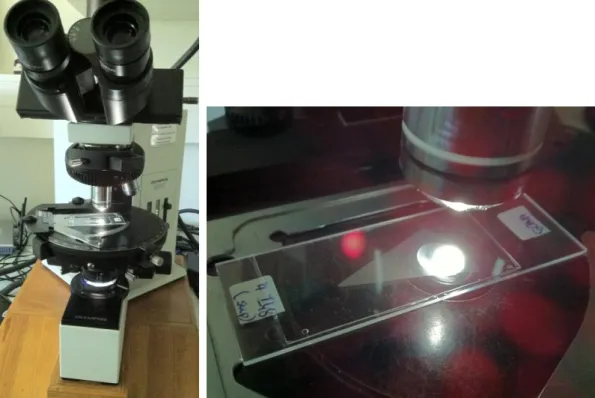
Figure 1: CTD sections off Loukkos river mouth. Stations where nannofossil analyses were performed are marked in magenta... 18 Figure 2– Photo of the Rosette coupled with the CTD equipment ... 19 Figure 3 – Coccolithophores counting using a petrographic optical microscope with the amplified

sample (FCUL- NannoLab). ... 22 Figure 4 – Sample view through petrographic optical microscope. The red arrows mark some

examples of cocoliths (a) and coccospheres (b) ... 23 Figure 5– Correlation between water turbidity in FTU measured by the nephelometer and SPM

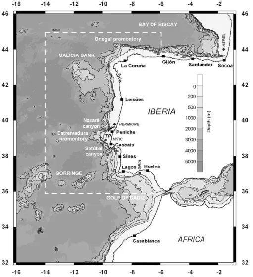
concentrations (g/l) determined in water samples. Color coding is used according to sampling depth. ... 24 Figure 6 – Previous numerical model domain (the West-Iberian Region). Global tide solutions were

forced at the open boundaries. These limits were selected in order to guarantee a homogeneous deep-ocean condition (distant from important topographic structures). Black squares indicate tide-gauges and gray circles the current-profile dataset locations, used to validate model results. The white dashed line delimits the study domain. Source: Quaresma and Pichon (2011) ... 26 Figure 7– Study area: Moroccan NW continental shelf with special focus on the Loukkos river area

of influence. (Source: Google Earth version 7.0.3.8542. 4b. Image date: 10/04/2013). . 27 Figure 8 - Larache and Loukkos river view from the sky.

Source:

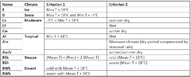
http://ancor.canalblog.com/albums/larache/photos/24709470-larache_map.html ... 28 Figure 9 – Continental shelf sedimentary facies cartography Source: DPDPM ... 30 Figure 10- Climate classification after a reduced Köppen scheme applied to the CRU TS2.1 data

(K. Born et al., 2008). ... 32 Figure 11– TS diagram showing the different water masses SW, SAW, NACW, MW and NADW from

all the stations of the Macroscale leg during GOLFO 2001 survey. (Criado-Aldeanueva et al., 2006). ... 33 Figure 12– Classical upwelling scenario in the Northern Hemisphere with a wind blowing along a

coast on its left. Source: W Peterson (1998). ... 34 Figure 13 - Upwelling regime in the NW African Coast (Moroccan coast).

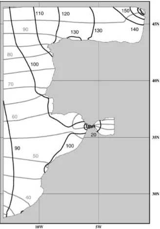
Source: Javier Arístegui (2009) and Hagen (2001). ... 35 Figure 14 – Amplitudes (black lines, in centimeters) and phases (grey lines, in degrees) of the M2

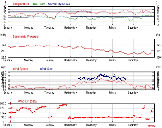
tidal constituent. Source: Fortunato et al. (2002) ... 36 Figure 15 – CTD station numbering scheme for cruise HM09 ... 45 Figure 16 – Meteorological conditions at Larache for the week of May 24th _{through 30} th_,2009

Source: WunderGround.com ... 46 Figure 17 – Meteorological conditions at Larache for the week of May 31th _{through June 6} th_,2009

4

Figure 18 – Meteorological conditions at Larache for the week of June 7th _{through 13}th_{,2009 Source:}

WunderGround.com ... 47

Figure 19 – Meteorological conditions at Larache for the week of June 14th _{through 20}th_,2009 Source: WunderGround.com ... 48

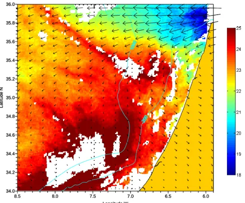
Figure 20 - Wind field and surface seawater temperature at 11th _{June 2009. Source: Martins and} Vitorino (2012). ... 48

Figure 21- Wind field and surface seawater temperature at 18th _{June 2009. Source: Martins and} Vitorino (2012). ... 49

Figure 22 – Tidal variability eclipses. Source: Martins and Vitorino (2012). ... 49

Figure 23 – 10 m deep current field, on the 21 June 2009, for the study area. Source: Martins and Vitorino (2012). ... 50

Figure 24 - TS diagram of sections 1 to 9 with the corresponding isopycnical lines. ... 51

Figure 25 – Temperature, salinity and density profiles for Station 141 (nearest station to Loukkos River inlet -section 5). ... 52

Figure 26 –Temperature, salinity and density profiles for Station 1 (offshore station of section 1). 53 Figure 27 – Temperature profiles measured on June 13 2009 in sections 1 and 2. ... 55

Figure 28 – Temperature profiles measured on June 14 2009 of sections 3 and 4. ... 55

Figure 29 – Temperature profiles measured on late June 14 2009 and in the early hours of June 15 2009 of sections 5 and 6. ... 56

Figure 30 – Temperature profiles measured on June 15 2009 of sections 7 and 8. ... 57

Figure 31 – Temperature profiles measured on June 15 2009 of section 9. ... 58

Figure 32 – Temperature distribution at 10 dbar represented for the entire study region. ... 59

Figure 33 – Temperature distribution near the bottom represented for the entire study region. ... 60

Figure 34 – Salinity profiles measured on June 13 2009 of sections 1 and 2. ... 61

Figure 35 – Salinity profiles measured on June 14 2009 of sections 3 and 4. ... 61

Figure 36 – Salinity profiles measured on late June 14 2009 and in the early hours of June 15 2009 of sections 5 and 6. ... 62

Figure 37 – Salinity profiles measured on June 15 2009 of sections 7, 8 ... 63

Figure 38 – Salinity profiles measured on June 15 2009 of section 9. ... 64

Figure 39 – Salinity distribution at 10 dbar represented for the entire study region. ... 65

Figure 40 – Salinity distribution near the bottom represented for the entire study region. ... 65

Figure 41 – Density profiles measured on June 13 2009 of sections 1 and 2. ... 66

Figure 42 – Density profiles measured on June 14 2009 of sections 3 and 4. ... 67

Figure 43 – Density profiles measured on late June 14 2009 and in the early hours of June 15 2009 of sections 5 and 6. ... 67

Figure 44 – Density profiles measured on June 15 2009 of sections 7and 8. ... 68

Figure 45 – Density profiles measured on June 15 2009 of section 9. ... 69

Figure 46 – Density distribution at 10 dbar represented for the entire study region. ... 70

Figure 47 – Density distribution near the bottom represented for the entire study region. ... 70

5

Figure 49 – Fluorometry profiles measured on June 14 2009 of sections 3 and 4. ... 72

Figure 50 – Fluorometry profiles measured on late June 14 2009 and in the early hours of June 15 2009 of sections 5 and 6. ... 72

Figure 51 – Fluorometry profiles measured on June 15 2009 of section 7 and 8... 73

Figure 52 – Fluorometry profiles measured on June 15 2009 of section 9. ... 74

Figure 53 – Fluorometry distribution at 10 dbar represented for the entire study region. ... 75

Figure 54 – Fluorometry distribution near the bottom represented for the entire study region. ... 75

Figure 55 – SPM concentrations profiles measured on June 13 2009 of sections 1 and 2. ... 76

Figure 56 – SPM concentrations profiles measured on June 14 2009 of sections 3 and 4. ... 77

Figure 57 – SPM concentrations profiles measured on late June 14 2009 and in the early hours of June 15 2009 of sections 5 and 6. ... 77

Figure 58 – SPM concentrations profiles measured on June 15 2009 of section 7 and 8. ... 78

Figure 59 – SPM concentrations profiles measured on June 15 2009 of section 9. ... 79

Figure 60 – SPM concentrations distribution at 10 dbar represented for the entire study region. ... 80

Figure 61 – SPM concentrations distribution near the bottom represented for the entire study region. ... 80

Figure 62 – Brünt-Väissäla frequency versus SPM concentrations for section 1... 82

Figure 63 – Brünt-Väissäla frequency versus SPM concentration for section 2. ... 82

Figure 64 – Brünt-Väissäla frequency versus nephelometry for section 3. ... 83

Figure 65 – Brünt-Väissäla frequency versus nephelometry for station section of section 4. ... 83

Figure 66 – Brünt-Väissäla frequency versus nephelometry for section 5. ... 84

Figure 67 – Brünt-Väissäla frequency versus nephelometry for section 6. ... 84

Figure 68 – Brünt-Väissäla frequency versus nephelometry for section 7. ... 85

Figure 69 – Brünt-Väissäla frequency versus nephelometry for section 8. ... 85

Figure 70 – Brünt-Väissäla frequency versus nephelometry for station section of section 9. ... 86

Figure 71 – Tidal Barotropic Forcing Term calculated for the study region. ... 87

Figure 72 – Nano concentrations vs. SPM concentrations. Orange squares represent the 5dbar coccolith samples; brown circles stand for lithos bottom samples. Coccospheres counted in the surface samples are represented in yellow while diatoms and dinoflagellates are represented by the cyan star. ... 88

7

Table Index

Table 1 - CTD sensors characteristics of General Oceanics MK IIIC of Instituto Hidrográfico (adap. 00201 MARK IIC/WOCE CTD UWV manual, 1994). ... 20 Table 2- Definition of classes of the reduced Köppen climate classification. T is the mean monthly

temperature in 2m height above ground, Prec is the annual precipitation sum. Max / Min T indicate the warmest and coldest month in the mean annual cycle. (K. Born et al., 2008)... 31 Table 3– Plankton classification - adapted from Oliveira (2001). ... 37

9

Acknowledgments

I wish is to thank to all who helped me and made this work possible, without them I could not have completed this thesis.

A special thanks to the Instituto Hidrográfico (IHPT) in person of Chief Director, Rear Admiral Silva Ribeiro, for all the facilities given that made this thesis realization possible since the beginning. I would like to thank the Marine Geology division, especially Aurora Bizarro that has given me the opportunity to work with and be part of so excellent team works.

I would like to thank Anabela Oliveira for her scientific orientation, critical judgement, friendship and good moments. A special thank to Ana Isabel Santos who helped me with her critical judgement pushing me to another level and for her friendship.

I would like to thank to João Vitorino for gently given me the treated data, essential to realization of this work, which without these I would never be able to complete it. I also would like to thank to Inês Martins who gently provided me important material of the study area.

I would like to thank to Lieutenant Luís Quaresma for his extraordinary help and information ceded on Internal Waves matter, crucial for this work development and conclusions.

I would like to thank Professor Mário Cachão for his scientific orientation and for helping me to start on Nannoplankton analysis.

I would like to thank the Faculdade de Ciências da Universidade de Lisboa, especially the Geology Department and Paleolab and Nannolab, for the facilities and conditions given.

I would like to thank to Diogo and his family, Laíse, mom and dad, my aunt Céu and my little cousins, Tiago and Tomás, for all the comfort and happy thoughts and for given me the strength to finish this thesis.

11

Abstract

In June 2009 Instituto Hidrografico (IHPT) conducted a multi-disciplinary survey of the NW Atlantic Margin of Morocco, onboard NRP “Almirante Gago Coutinho” (cruise HM09). This cruise served several objectives and was integrated by project HERMIONE and by a project of cooperation between Portugal and Morocco. During this cruise, CTD (Conductivity, Temperature and Depth) observations were performed across nine sections in the inner/middle Moroccan shelf, off the Loukkos river mouth, perpendicular to bathymetry orientation.

The multidisciplinary work aims to understand and explain the prevailing physical processes and sediment dynamics at the inner/middle continental shelf adjacent to the Loukkos river mouth and basin. This work main objective is to infer a conceptual dynamic model of the study region, considering local and seasonal events, observed during the cruise time (summer time).

Since ocean dynamics are not strictly physical, geological or biological but, instead being the result of several and different processes, diverse methodologies were used since CTD data acquisition to data treatments. Physical variables, such as temperature, salinity, density and Brünt-Väissäla Frequency were treated as geological and biological approaches (Suspended Particulated Matter; Chlorophyll-a concentrations analysis and nannoplankton couting) were also considered.

Nannoplankton, here used as water masses tracer, also gave crucial information about the ocean dynamics (resuspension and water column transport). Using the (cocco)liths versus (cocco)spheres model, it was possible to infer bloom and decline phases of the most important species present in the study area.

Results show that the observed locally changes on wind field direction and intensity changed oceanic dynamics, causing locally cyclic upwelling events with alternation between mature upwelling state and less intense upwelling conditions. The study region is also under the influence of IWs propagation over the slope and shelf. These features deeply affected the water column, being strongly energetic to resuspend the bottom sediments, which is coherent with the existence of BNL and SNL found in the SPM concentration analysis. Concentration analysis also shows that the most affected area by the IWs is the inner/mid-outer shelf boundary, with higher values of SPM concentrations, since easily removed, very fine and well-sorted sediments compose this area. In the other hand, chlorophyll-a results are in conformity with the Navarro et al. (2006) model, being closely related with the 26.66 kg.m-3 _{isopycnical, which marks the initial location where the}

maximum nutrient gradient is when the spring-summer season begins.

13

Resumo

Em Junho de 2009, o Instituto Hidrográfico organizou um cruzeiro multidisciplinar no Atlântico ao longo da margem da costa NW Marroquina, inserido no projeto europeu Hermione, a bordo do NRP “Almirante Gago Coutinho”. Durante este cruzeiro, foram realizadas medições de CTD ao longo de 9 secções perpendiculares à batimetria, constituídas por 73 estações, distribuídas ao longo da plataforma continental marroquina e próximas da embocadura do Rio Loukkos. Foram feitas colheitas de água junto á superfície (aos 5m) e junto ao fundo que foram, posteriormente, filtradas para análise. A área de estudo encontra-se entre as latitudes 34° N e 35.5° N, localizada entre as zonas áridas do deserto do Sahara e as regiões moderadas do Mediterrâneo e Atlântico. É uma zona de clima moderado com uma estação seca de verão (mediterrânica com influência oceânica), caracterizada por taxas elevadas de evaporação e baixos valores de precipitação. O estuário do Loukkos é um dos maiores estuários de Marrocos, que devido ao seu caudal (valor médio aproximadamente 500 ls-1_{), gera uma vasta atividade económica ligada à agricultura.}

Na plataforma interna–média, a profundidades inferiores a 50 m, constituindo o prisma de acreção continental é possível encontrar um depósito de areias terrígenas, muito bem calibradas e finas. A plataforma média-exterior, entre os 55 – 120 m de profundidade, é constituída por um depósito lodoso muito bem calibrado.

As medições foram efectuadas de 13 a 15 de Junho de 2009, em que as condições meteorológicas observadas, na semana anterior à do cruzeiro e nos primeiros dias deste, eram de vento estável e predominantemente do quadrante norte (favoráveis ao upwelling) com intensidades rondando os 30 km/h. No entanto, durante o cruzeiro, foram registadas pequenas flutuações no campo de vento para sul com uma pequena atenuação na intensidade do vento nos dias 31 de Maio, 2, 7 e 9 de Junho. Martins & Vitorino (2012) usaram medições efectuadas por correntómetros e perfis de CTD para caracterizarem o padrão de circulação sub-inercial da margem NW marroquina. O padrão complexo de circulação de superfície mostra uma corrente N-S paralela e junto à costa e a interação da recirculação da corrente dos Açores com o jacto de upwelling. A zona de estudo é dominada pela componente semi-diurna da maré (M2). No que diz respeito às massas de água, sendo as medições efectuadas apenas na plataforma continental até uma profundidade aproximada de 220 m, a única massa de água propriamente dita presente na área de estudo é a North Atlantic Central Water (NACW). Nas camadas superficiais é ainda possível distinguir-se duas “massas de |gua” com características distintas, Surface Atlantic Water (SAW), resultante da modificação da NACW por interações ar-oceano e a Warm Shelf Waters (SW) resultante da SAW e influenciada por processos da plataforma continental como aquecimento e inputs de água doce.

Para a realização deste trabalho foram tratados dados de temperatura, salinidade, densidade, frequência de Brünt-Väissäla, nefelometria, fluormetria recorrendo ao software Grapher 9.0 e

Surfer 8.0 (Golden Software). Determinou-se a correlação entre os resultados de nefelometria

14

filtragens realizadas ao longo da coluna de água, utilizando como resultados os valores da concentração de matéria particulada em suspensão na coluna de água (SPM – suspended particulate

matter concentrations).

A contagem de nanoplâncton, de 6 estações estrategicamente escolhidas, foi realizada utilizando os filtros de superfície e junto ao fundo e recorrendo a um microscópio petrográfico no NanoLab da FCUL.

Os resultados obtidos de temperatura, densidade e salinidade mostram que, devido às oscilações meteorológicas observadas a área de estudo, esta esteve sobre a influência de eventos cíclicos de

upwelling, com a alternância entre estados maturos e upwelling menos intenso. Não foi possível

observar-se a assinatura do Rio Loukkos na bacia oceânica adjacente já que o seu caudal, além de controlado por barragens, nesta estação do ano, é fortemente reduzido devido à elevada taxa de evaporação e à quase não ocorrência de eventos pluviosos, características do clima da região. As estações 1, 2 e 5 registaram um evento de upwelling maturo com o jacto de upwelling a chegar à superfície, interrompendo-a, e deflectindo para offshore a água das camadas superficiais.

Nas restantes estações, verificou-se uma atenuação do estado de upwelling com a presença do jacto a ascender à superfície, contudo, sendo observado a profundidades superiores. Este enfraquecimento está inteiramente ligado à deflexão do campo de vento para S-SW (direcção não favorável) e ao decréscimo da velocidade do vento.

Estando esta área em particular da costa NW marroquina inserida ainda na Westerly Wind Zone (zona de ventos predominantes de Oeste), as condições para a formação e duração de eventos de

upwelling são muito similares às observadas na costa Portuguesa, com a exceção de que na bacia

oceânica adjacente ao Loukkos, no verão, não é possível observar-se a assinatura fluvial do rio Loukkos.

Esta região está, ainda, sobre a influência de ondas internas e da sua propagação na vertente continental, assim como na plataforma continental, que origina pulsos de correntes com velocidades suficientemente elevadas capazes de resuspender os sedimentos de fundo. As ondas internas são facilmente detectadas nos perfis de temperatura, salinidade, densidade e, particularmente, no perfil de clorofila-a (perfil de fluorometria) onde as camadas de água aparentam uma forma ondulatória.

Os resultados de concentração de SPM relevaram a presença de uma camada nefeloíde de fundo, em toda a zona de estudo, desde os 20 m de profundidade até aos 120 m, aproximadamente, compreendo a plataforma interna-média e a plataforma média-exterior. Valores máximos de matéria particulada em suspensão foram observados na fronteira entre estes dois depósitos sedimentares já que esta é constituída por depósitos muito finos e bem calibrados, facilmente remobilzados e transportados na coluna de água. É também possível observar-se uma camada

15

nefeloíde de superfície, localizada junto e ao longo da linha de costa, com valores inferiores de SPM, possivelmente relacionados com o jacto de upwelling.

Apesar de as colheitas de água não ter sido realizadas a profundidades ideais para a análise de nanoplâncton, os resultados obtidos demonstram, de uma maneira geral, que as espécies dominantes eram E. huxleyi e G. muellarae e, que na altura da colheita, existiam litos em maiores quantidades do que cocosferas da respectiva espécie. Foi possível também depreender que as espécies E. huxleyi e G. muellarae se encontravam em bloom enquanto que a espécie G. ericsonii estava, muito certamente, numa fase de declínio.

17

Chapter 1: Introduction and Objectives

Underneath the waves our seas are home to some of the most spectacular ecosystems on Earth. Ecosystems such as cold-water coral reefs and hydrothermal vents support a huge diversity of life that is both beautiful and alien, but also vulnerable to the impacts of climate change and human activities. The European HERMIONE project focused on investigating these and other ecosystems, including submarine canyons, seamounts, cold seeps, open slopes and deep basins. Scientists from a range of disciplines researched their natural dynamics, distribution, and how they interconnect. The scientists also wanted to find out how these ecosystems contribute to the goods and services we rely on, and how they are affected by natural and anthropogenic change. A major aim of HERMIONE was to use the knowledge gained during the project to contribute to EU environmental policies. This information can be used to create effective management plans that will help to protect our oceans for the future. (http://www.eu-hermione.net/)

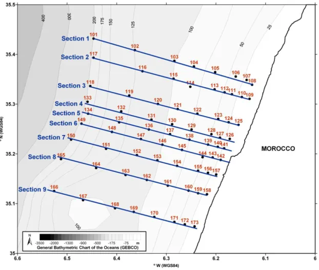
In June 2009 Instituto Hidrográfico (IHPT) conducted a multi-disciplinary survey of the NW Atlantic Margin of Morocco, onboard NRP “Almirante Gago Coutinho” (cruise HM09). This cruise served several objectives and was integrated by project HERMIONE and by a project of cooperation between Portugal and Morocco (FCT/CNRST). The NW Moroccan continental shelf was soon recognized by HERMIONE partners as an area of interest, due to its close affinity to the Iberian shelf and its proximity to the Gulf of Cadiz. One of the main goals of the work program was to characterize the different physical processes that act on the Moroccan continental slope and adjacent shelf, in the area of the El-Arraiche Mud Volcano field, during summer. During this survey, one of the components included CTD (Conductivity, Temperature and Depth) observations in nine sections in the inner/middle Moroccan shelf, off the Loukkos river mouth, perpendicular to bathymetry orientation (Figure 1).

The main objective of this survey was to understand and observe the prevailing physical processes and sediment dynamics at the inner/middle continental shelf adjacent to the Loukkos river mouth and basin. However, this particular thesis is a Master’s degree final project in the area of Ocean Sciences, a multidisciplinary course. Therefore, it has several implicit objectives inherent to the master's program itself, such as the studying of several fields of expertise and the crossing of different types of data and data management and processing. As a result, in order to understand the pattern of the suspended particulate matter (SPM) in the water column or the processes involved in bottom sediment ressuspension, both coccolithophore and diatomaceous species were considered for water masses tracing; as proxies of SPM dynamics. Nannofossil data will be used to corroborate bottom sediment resuspension processes observed in CTD data (nephelometry/turbidity and with water column content in chlorophyll-a/fluorometry).

18

Figure 1: CTD sections off Loukkos river mouth. Stations where nannofossil analyses were performed are marked in magenta

In the second chapter of this thesis the methods used to collect, process, present and analyse data will be described. In the regional settings chapter (third chapter), a characterization of the Loukkos basin and the adjacent continental region is presented, as well as the Loukkos flow regime, local and regional climatology and atmospheric forcing. In the fourth chapter, pertinent data from the HM09 cruise will be presented and discussed that will show the main results of this work, namely: physical data profiles (for each station), nephelometry vs. Brunt-Vaissala frequency graphics; as well as results obtained through nannofossil proxy data. Finally in the last two chapters, the main conclusions of this work are presented, as well as some remarks about future work in this area.

19

Chapter 2: Methods

I - Data collection

Physical data (Conductivity, Temperature, Depth, nephelometry and fluorometry) was collected on board hydrographic vessel “NRP Gago Coutinho” using a Neil Brown General Oceanics MK IIIC CTD

probe, coupled with an Aquatracka nephelometer (water turbidity) and a Seapoint flurometer (device that measures the chlorophyll-a content in water), amongst other types of data collection since HM09 cruise 2009 had broader objectives than those discussed in this thesis. Loukkos CTD data and water sampling took place between 13 and 15 of June 2009. Water sampling for SPM collection was performed using 12 Niskin bottles (8l each), coupled to a Rosette sampler Physical data were collected during CTD probe descent. At the same time, this data was being plotted and visualized in real time, which allowed for CTD operators to decide at which levels water samples should be collected. The sensors characteristics, such the range of work and their precision and resolution, are shown in Table 1 and Figure 2.

r– Rosette with the 12 Niskin bottles; c – CTD equipment;

n – Nephelometer.

20

Table 1 - CTD sensors characteristics of General Oceanics MK IIIC of Instituto Hidrográfico (adap. 00201 MARK IIC/WOCE CTD UWV manual, 1994).

Sensors Range of Work Resolution Precision Pressure (dbar) 0 – 7000 0.0015% 0.0014% Temperature (C) -3 – 32 0.0005 ± 0.002 Conductivity (mS cm-1_{) 0 – 70 0.001 ± 0.002} Nephelometry (FTU) 0-10 – ± 0.01 Fluorometry (μg/l) 0 – 15 – ± 0.02

II -

CTD data processing

CTD raw data is obtained with the General Oceanics firmware. These data are saved in binary format files and converted into ASCII format. At Instituto Hidrográfico (IHPT) the procedure to process, calibrate and calculate derivate physical variables has been implemented having the UNESCO recommendations as the point of start (Silva et al., 1992). Steps to process and calibrate CTD data can be summarized as follows:

I. The conversion of the binary files into ASCII files (type *.dat) using the previously determined calibration constants obtained in laboratory for all the different sensors (except for the nephelometer);

II. Pressure offset definition (value, different from zero, registered before putting the equipment under water) and exclusion of impossible data;

III. Insertion of administrative data (for ex: name of the cruise; time and depth); IV. Descending speed calculation as a function of the pressure channel;

V. Application of a recursive filter in the temperature and conductivity channels in order to correct the sensors response times according to of the descending speed;

VI. Rectification of the conductivity channel for the temperature and pressure effects in the water column;

VII. Use of in situ calibration constants;

VIII. Application of nephelometer calibration constants (conversion of volts to FTU – formazine turbidity units);

IX.

X.

temperature, geo-potential anomaly referred to the surface, speed of sound and depth in meters.

21

III -

Water Samples – SPM determination

Water sampling and filtration were performed on board of the NRP “Almirante Gago Coutinho”. Sampling and filtration procedures on board have been previously described by Oliveira (1994, 2001). Briefly, surface water (5m) was collected using a suction pump, and below surface waters were collected using the Rosette sampler. 47 mm cellulose acetate filters were used, with a 0.45 µm mesh according to the general understanding that any particle < 0.45 µm is considered as dissolved. Volume of water samples was always in the order of the 5-10 liters.

A - Laboratory work

1. SPM concentration (mg/l)

Filters used for SPM sampling were pre-weighed before the survey preparation, involving a highly laborious laboratorial process. In order to obtain a precise measure of filter mass, it is necessary that the filters are perfectly dry and at room temperature. For that, the unused filters were placed in a stove at constant temperature of 40C during 24h. After this period, they are left to cool inside desiccators in order to prevent water absorption. After sample filtration onboard, the same procedure is used to obtain filter + SPM mass.

The following relation is used to determine SPM concentrations (mg/l):

(Equation 1) Where:

 Wf– Final weight of the filter;

 Wi– Initial weight of the filter;

 V – Volume of filtered water.

2. Coccolithophore species counting

Coccolithophores are carbonated fossils (generally calcite) with dimensions under 20



Calcareous nanofossils, used as water masses proxies, were counted in order to understand which were the main species present in the study area and to infer the SPM origin in the water column. Sampling was made at two depths: near the seabed and at 5m water depth, near the surface layer. Six CTD stations were chosen to nannoplankton accounting: two from the first section on the

22

northern sector of the study area, two from the section in front of Loukkos River inlet and another two of the southern section.

For coccolithophore concentration determination, a small sector of each SPM filter was used, both from the surface and bottom samples for the selected CTD stations. The coccolithophore analysis was performed at the Faculdade de Ciências da Universidade de Lisboa, FCUL, in a specialized laboratory – the “NanoLab” (Figure 3 and Figure 4).

The assemblies were prepared using one slide and one cover-slip per filter, where each filter was placed between the slide and the cover-slip, wrapped in Entellan – a synthetic balsam that is used to improve the optical continuity (Figure 3).

The amount of coccolithophores was determined using a petrographic optical microscope with crossed poles. The choice of using this type of instrument is that any crystal matter, as calcite, will be bright when observed with the crossed poles, facilitating the coccolithophores’ observation and count. A quantitative analysis was made for the actual species, while the remobilized nannoplankton were only considered qualitatively.

In the surface samples, dinoflagellates and diatoms were also considered to counting but without specie differentiation.

In order to infer the relation between the nannofossil species presented in the study area with SPM concentration, for the surface and bottom samples in separate, a linear regression was calculated, using Grapher software 9.0.

Figure 3 – Coccolithophores counting using a petrographic optical microscope with the amplified sample (FCUL- NannoLab).

23

Figure 4 – Sample view through petrographic optical microscope. The red arrows mark some examples of cocoliths (a) and coccospheres (b)

3. Cocospheres vs. coccolith model

For a more detailed nannoplankton analysis, the results of the accounted species were processed statistically using MO Excell program. Coccoliths amount in coccoliths.l-1_{, medium and standard}

deviations were calculated to understand and infer the ecologic performance of the envolved species.

It was also applied the the model developed by Cachão and Oliveira (2000), using data from the CORVET (Corrente da Vertente) cruise, carried out off the western portuguese coast in November 1996 by IHPT, to comprehend and recognise ecological performance, i.e., when a particular specie is blooming, when it is in a steady developing state, or when it is in a decay processe (for more detail information please consult in Cachão and Oliveira, 2000. (Cocco)liths versus (cocco)spheres:

Aproxing the ecological performance of coccolithophores.).

IV -

Nephelometry data – FTU to inferred SPM concentration

a

24

the same type of material. Therefore, disperse light intensity will give us a measurement of the relative content of particles in a determined level (Durrieu de Madron et al., 1990).

The nephelometer was previously calibrated using a standard formazine solution. During this calibration an exponential relation was found between nephelometer output in Volts and Formazine Turbidity Units (FTU). This relation was used during CTD processing in order to covert Volts to FTU.

A - Relation FTU vs. SPM concentration

The conversion of the nephelometry in FTU into SPM concentration (mg/l) was determined in order to infer SPM concentrations in continuous fields. Nephelometry data and SPM concentrations were correlated for the sampling levels. After eliminating remarkable outliers the following relation was found (Figure 5 and (Equation 2). The distribution shown in Figure 5 reinforces sample distribution differences, possible due to different sediments and materials in suspension.

(Equation 2)

Figure 5– Correlation between water turbidity in FTU measured by the nephelometer and SPM concentrations (g/l) determined in water samples. Color coding is used according to sampling

25

V -

Barotropic tide modelling

In similarity to what was done by Quaresma and Pichon (2011) in “Modelling the barotropic tide along the West-Iberian margin”, a numeric model was used to predict the barotropic tide along the coast adjacent to the Loukkos River inlet. The HYCOM model (Hybrid Coordinate Ocean Model) was used, in a single ispycnal layer, to simulate the 2D propagation of the following eight principal tidal constituents: M2, S2, N2, K2, K1, O1, P1 and Q1. Recently updated global tide solutions were optimally combined to force a polychromatic tidal spectrum at the open boundaries, where the eight principal constituents were assembled and forced at the open boundaries. This option allows non-linear harmonic interactions in the resulting solution, as expected in nature. The presented model outputted an absolute tidal solution and its evaluation was performed by harmonic analysis. Higher accuracy was achieved by adding the astronomical tide-raising force into HYCOM momentum equations and by improving the bathymetry information over the region. Self-attraction/loading (SAL) terms were not included, based on the principle that they are negligible near coastal regions and that the utility of using them is questionable (Ray, 1998). In order to validate both sea-surface height and tidal current velocity solutions, as done by Pichon and Correard (2006), accurate barotropic tidal ellipses simulations were also done, enabling better estimations of the tide generation forcing term (Quaresma and Pichon; 2011).

For tidal forcing calculus, regional circulation numerical models by boundary conditions forcing. The sea-surface elevation and the corresponding 2D velocity components are imposed as tidal harmonics along the open limits. Quaresma and Pichon (2011) use two recently revised and updated global tide solutions: TPXO7.2 and NEA2004 Tidal Atlas. Each results from different modelling approaches.

TPXO7.2 is the most recent solution of the OTIS model (Egbert et al., 1994) that best fits the Laplace tidal equations to altimetry data from TOPEX/Poseidon plus Jason (since 2002 until present). The North-East Atlantic tidal atlas (NEA2004) results from a regional nesting of FES2004 (Lyard et al., 2006), carried out by the Toulouse Unstructured Grid Ocean model (T-UGOm) in a 2D barotropic, shallow water mode (Pairaud et al., 2008). FES2004 is also a global tide hydrodynamic model, improved by tide-gauge and altimetry data assimilation (TOPEX/Poseidon plus ERS-2).

The two global solutions were introduced, one at a time, as HYCOM's open boundary conditions. The adopted polychromatic solution, used as boundary conditions in the present HYCOM configuration, resulted from the assembling of N2, M2 and S2 constituents from NEA2004 and K2, Q1, O1, P1 and K1 from TPXO7.2.

26

The gravitational tidal gradient force, ∂P/∂x and ∂P/∂y, was added to HYCOM barotropic momentum equations (1), as:

(Equation 3) Where CL is the moon's reference potential (0.2687536 × 10−3 _{km), φi a latitude coefficient, Di the}

Doodson coefficient for each constituent (i) and αi, bi the respective nodal corrections parameters.

Figure 6 – Previous numerical model domain (the West-Iberian Region). Global tide solutions were forced at the open boundaries. These limits were selected in order to guarantee a homogeneous deep-ocean condition (distant from important topographic structures). Black squares indicate

tide-gauges and gray circles the current-profile dataset locations, used to validate model results. The white dashed line delimits the study domain. Source: Quaresma and Pichon (2011)

27

Chapter 3: General environmental overview and regional

settings

I - Study area

The study area lies between the latitudes of 34° – 35.5°N, comprising an area of the Moroccan continental shelf under the direct influence of the Loukkos river discharge (Figure 7).

Figure 7– Study area: Moroccan NW continental shelf with special focus on the Loukkos river area of influence. (Source: Google Earth version 7.0.3.8542. 4b. Image date: 10/04/2013). In order to characterize this area, it is crucial to enumerate some of the most important aspects that distinguish the NW African coast. Geological settings, geomorphological characteristics, regional hydrology, the relation between circulation patterns and atmosphere forcing as well as spatial distribution of productivity proxies such as chlorophyll and diatoms are some of the main features referred and studied in this report.

The study area is located, as it was mentioned before, in front of the Loukkos River inlet. The continental adjacent region is highly populated since there is an important harbor town – the city of Larache, which belongs to the region of region Tanger-Tétouan in northern Morocco (Figure 8). The Province of Larache covers a surface around 2 783 km². Its population is of order of 431 476 (Census of 1994), including 201 485 in the urban communes and centers, and 229 991 in the rural communes. The urbanization rate is proximally 46.7%, with a population density of 155 habitants/km².

28

Figure 8 - Larache and Loukkos river view from the sky.

Source: http://ancor.canalblog.com/albums/larache/photos/24709470-larache_map.html

II -

Loukkos River

The Loukkos river estuary, one of the major estuaries of Morocco, is located on the Atlantic coast of Morocco delimited between 35° 09' and 35° 14' N and 006° 05' and 006° 30' W (El Morhit, 2009). Loukkos is one of the most important rivers in Morocco mainly due to its important flow values, resulting in vast agricultural and economic activity. The Loukkos hydrographic basin extends over an area of 3.740 km2 _{and, topographically, it is characterized by a very flat lower valley}

(10-15 masl- meters above sea level), with a negligible slope (actually, 44 km upstream the river mouth, the bottom is even below sea level). The main channel depth varies from 2 to 4 m but in some places it may reach 15 m (Snoussi, 1980). In the Loukkos basin, the estimated average annual rainfall is 700 mm. (El Gharbaoui, 1981). The hydraulic network of the Loukkos perimeter is formed by surface waters of the Loukkos river and its tributaries (Drader, Soueir, Skhar and M’da), and its drainage is characterized by an irregular interannual regime: the lower flow values are generally null, except from streams that drain the water from R’Mel (Sakhsokh, Smid El Ma and El Kihel) with an average flow of 500 ls-1 _{and those draining the water from Drader-Souiere. The}

mesotidal Loukkos estuary (tide: 3.5m, semi diurnal) is a tide-dominated system, according to the classification of Dalrymple (1992). This estuary is currently in a filling phase that occurred during the Flandrian (Mellahian) transgression and, more recently, by the progression of the sandy spit (Aloussi, 2008 and Carmona, 2009). This sandy spit supports the fast sedimentation of fine particles (silt and clays) and also of sand (Palma et al, 2012).

III -

Quaternary evolution and actual continental shelf

Sedimentary Facies

During the Quaternary, in the Atlantic Morocco the glacial-eustatic movements resulted in several transgressions of varying amplitudes, with the formation of mixed cobble sized deposits with lumachelles and the occasional cliffs. Glacial events significantly lowered the sea level, while post Villafranchian transgressions caused a small rise in sea level. The actual deposits’ altitude depends

29

almost exclusively on epeirogenetic phenomena acting on this coastal sector. The several marine transgression episodes allowed the accumulation of sand, gravels and shelly deposits on the shore. In the succeeding regression these shelly-sandy beaches were reworked into dunes parallel to the shore and later consolidated in oblique, cross-bedded and covered strata of calcareous sandstone that was later covered by continental deposits. The exact sea-level reached after the Villafranchian transgression is marked by polished-base cliffs. The local climate changes that accompanied glacial eustatic events correspond to alternation of rainy intervals (cooler, wet weather) with warmer and drier weather intervals.

Currently, according to Oliveira et al. (2010), the main amount of sediments and SPM present in the study area comes from Loukkos River. The estuary’ sediments are composed mainly by fine particles and, in the lower estuary, by some sandy carbonated sediment (Figure 9).

According to figure Figure 9, three sedimentary deposits can be identified in the continental shelf: the first one is a sandy inner mid-shelf deposit (<50m depth) with very fine and well sorted terrigenous sand, but where poorly sorted sands also can be found, formed predominantly by terrigenous sediments (quartz, mica and rock fragments, mainly calcarenite). These sands constitute the coastal accretionary prism. Hasnae and Abdou, (2007) also indicated a terrigenous sands deposit that occupy the internal flat shelf between the coastline and the 50 m isobaths. Secondly, a mid-outer shelf muddy area (55 – 120 m depth) is found, formed by very well sorted muds. Further offshore, an outer shelf deposit with very poorly sorted and polymodal very fine biogenic sand is found, occupying a relatively narrow band on the outer edge of the shelf. These are characterized by high carbonate content, generally higher than 50% and locally reaching 70%. The carbonate phase is essentially biogenic. Bioclastic elements are difficult to identify because they are often broken, damaged and oxidized. These sands have some similarity with the sands studied onshore, in the region of Larache (Adil Said 1996). Macro-fauna is mainly represented by fragments of bivalves and gastropods and, in a less relevant number, by fragments of Echinoderms, Bryozoa, Dentalium, brachiopods and sponge spicules. Micro-fauna consists mainly in planktonic and benthic foraminifera and ostracod shells. Quartz, calcarenite fragments and micas represent the terrigenous fraction as well as glauconitic and phosphate components, reflecting the character of an open depositional environment.

The X-ray diffraction analysis of shelf sediments shows a complex association of minerals. The dominant mineral is calcite with an average content of 63% (min: 42%, max: 72%), followed by quartz, (average 12%, min: 5%, max: 21%), the other minerals (dolomite, phyllosilicates, plagioclase, opal C/CT, siderite and pyrite) are present but in smaller proportions (<10%). Grain-size and mineralogy seem to indicate different sources of terrigenous sediments to the shelf in front of Loukkos and also the Sebbou rivers, and also different interconnectivity between river/shelf systems. In the Loukkos some marine influence is found in the lower estuary (richer in biogenic sand component) decreasing upstream. (Oliveira et al., 2010).

30

Figure 9 –Continental shelf sedimentary facies cartography Source: DPDPM

IV -

Atmospheric Forcing

As far as the atmospheric forcing is concerned, the Moroccan margin is, in large scale, affected by the seasonal fluctuations of the North Atlantic subtropical gyre. The size and position of this gyre follows the movements of the Azores atmospheric high, which extends northwards in summer and reduces its size in winter. Following these oscillations, the Azores current flows to latitudes higher than the Gulf of Cadiz (GoC) in summer, and it is displaced southward in wintertime. This seasonality deeply affects the surface circulation along the eastern boundary of mid-latitude North Atlantic (García Lafuente and Ruiz, 2007). Nevertheless, the prevailing winds are westerly (around 63%; Aberkan, 1989), particularly during the winter period, while during summer persistent northeasterly tradewinds are observed. Besides large-scale events, the Moroccan coast is also

31

affected by intermittent wind forcing, which has an important influence in the local circulation, resulting in localized events, such as coastal upwelling, currents and waves.

V -

Climatology

Morocco is located between the arid regions of the Western Sahara and the moderate Mediterranean and Atlantic regions. Landscape types reach from flat areas in the north-western part to high- mountain areas in the Atlas and Rif. Therefore, a large variety of climates can be found, ranging from moderate humid and sub-humid climates at the northern slope of the High Atlas, to semi-arid and arid climates south of the Atlas.

According to the reduced Köppen climate classification (Table 2), the study area is classified as Cs: moderate climate with a dry summer season (Mediterranean with an oceanic influence) (Figure 10 and Table 2). Dry seasons are known for the high evaporation rates and for low river discharges to ocean.

Table 2- Definition of classes of the reduced Köppen climate classification. T is the mean monthly temperature in 2m height above ground, Prec is the annual precipitation sum. Max / Min T indicate

32

Figure 10- Climate classification after a reduced Köppen scheme applied to the CRU TS2.1 data

(K. Born et al., 2008).

VI -

Regional Hydrology

Despite of the maximum depth of the discussed data sets being approximately 220 m; the extended knowledge of the different water-mass present in the Moroccan margin is essential to understand the full dynamic mechanisms that result from their interplay (Figure 11).

Surface Atlantic Water (SAW) makes up the layers near to the surface. This layer has its origin in shallow North Atlantic Central Water (NACW hereinafter), modified by air–sea interactions (Criado-Aldeanueva et al., 2006). In some cases, water warmer and fresher than SAW has been detected in the surface, mainly over the continental shelf. These Warm Shelf Waters (SW) results from SAW that has been noticeably influenced by continental shelf processes, including heating and fresh water inputs from land (Criado-Aldeanueva et al., 2006).

Immediately below the SAW, the NACW widens to a salinity minimum that can reach 600-700 m depth in some southeastern regions. This water mass is characterized by nearly horizontal isohalines (Tomczak, 1981). The NACW has a linear behavior in a temperature vs. salinity (TS) diagram and ranging between the values of 11.0C ≤T≤ 17. 0C; 35.6 ≤S≤ 36.5 and 26.6 kg.m-3 _≤γθ≤

27.3 kg.m-3 _{(Knoll et al., 1999 and Ambar et al., 2002). This water mass has been subdivided by}

some authors between subtropical and subpolar NACW, according to its origin (Harvey, 1982; Pollard and Pu, 1985; Pérez et al., 2001). It is considered that the upper 500 m are taken by the subtropical NACW whereas the subpolar NACW lies between 500 to 700 m depths.

33

In the intermediate layers (600 to 1500 m depth) two different water masses can be recognized: the Mediterrean Water (MW hereinafter), characterized by its high salinity (35.5) and the Antarctic Intermediate Water (AAIW hereinafter), characterized by salinity values under 35.3 (Hernández Guerra et. al., 2001).

Bellow 1500 m depth, the deep layer is composed by the North Atlantic Deep Water (NADW) that is characterized by a decrease in salinity with depth and the near horizontal isohaline distribution (J.L. Pelegri et al., 2005).

Figure 11– TS diagram showing the different water masses SW, SAW, NACW, MW and NADW from all the stations of the Macroscale leg during GOLFO 2001 survey. (Criado-Aldeanueva et al., 2006).

VII -

Circulation Pattern

The surface circulation in the NW African Coast is linked to the northeastern branch of the North Atlantic gyre formed by the Azores current, which is a zonal meandering flow that stretches across a large extent of the North Atlantic, and equatorward, slowing moving Canary current (J. García Lafuente and J. Ruiz, 2007).

The Gulf of Cadiz (GoCis) morphology is crucial to the Azores current’s formation, to the “feeding the inflow of Atlantic water into Mediterranean Sea and to the presence of the Mediterranean water energetic plume (Jia, 2000; Johnson and Stevens, 2000). The surface circulation of NW African coast is sensitive to seasonal variability in large-scale events, as previously described in this chapter. Relvas and Barton (2002) proposed that, when the upwelling jet formed in summer reaches in Cape San Vicente (Portugal), it spreads preferably to the east along the shelf break and slope of the northern part of GoC, providing a generalized anticyclonic circulation in the basin. Part of the flow entering the GoC feeds the Atlantic surface inflow into Mediterranean Sea and part recirculates

34

anticyclonically to merge with the Azores and Canary currents further south (J. García Lafuente, J. Ruiz.,2007). In conclusion, the NW African coast has an unique anticyclonic circulation pattern - where Atlantic water inflows to the coastal zone. Additionally, during the summer, wind fields blowing from NW, along the Moroccan coast, promote the formation of upwelling jets, Ekman layers and currents (Figure 12).

Figure 12– Classical upwelling scenario in the Northern Hemisphere with a wind blowing along a coast on its left. Source: W Peterson (1998).

The depth-averaged currents called the Ekman drift form a 90° angle with the wind to the right in the Northern Hemisphere, according to the simple theory. When the wind blows along a coast on its left in the Northern Hemisphere, it generates offshore Ekman drift. Water deflection occurs in the upper layers, and a low pressure sets in, forcing waters from below to move upward and replenish, at least, part of the space vacated by the offshore drift. To complete, a wind blowing along shore provokes an offshore current at upper levels, upwelling at the coast and an onshore current at the lower depths. This phenomenon is called coastal upwelling. The intensity of the wind will dictate the upwelled state. After a weak or brief wind, the interface has upwelled but not reached the surface while in the case of strong or prolonged wind events cause the interface to reach the surface, where it forms a front, which is displaced offshore, leaving the cold waters from below exposed to the surface. This last case corresponds to a mature upwelling that favors biological activity. The coastal upwelling area off NW Africa is one of the four large upwelling systems of the Eastern Boundary Currents, within the trade wind belts of the subtropics (EBC) (Hagen, E., 2000).

35

Figure 13 - Upwelling regime in the NW African Coast (Moroccan coast). Source: Javier Arístegui (2009) and Hagen (2001).

The study area is located above the Easterly winds zone and belongs to the Westerly wind zone, the same wind zone where the Portuguese basin is located. Consequently, the main trade winds are from NW quadrant. Moroccan upwelling system has some similarities with the classical upwelling regime: Equatorward wind stress, represented by small circles, provokes offshore transport (grey arrows) in surface Ekman layer, comprehended above dashed blue line, which are replaced by onshore flow (black arrows) in and below the upwelled pycnocline (green), and an equatorward jet (red), above a poleward flow (blue) trapped to the continental slope. In the bottom Ekman layer (below dashed blue line near seabed) flow will have an offshore component below poleward flow (Javier Arístegui, 2009). Nevertheless, the main difference between the Moroccam upwelling regime and the classical regime is that Moroccan wide shelf upwelling may separate from coast where surface and bottom Ekman layers merge (Figure 13). As Figure 13A shows a comparison between Portuguese and Moroccan typical scenarios. The difference can be found only near the coast, where the Portuguese coast has a weak poleward flow in opposite to what is observed in the Moroccan coastline, where an inner shelf mixed zone can be found. However, in the particularly study region, continental shelf width is similar to the Portuguese one, therefore there will expected to found comparable upwelling conditions in both continental shelves.

As the discussed data set only range approximately 220m depth, it is only possible to observe the near surface circulation. Summarizing, the circulation patterns are the response to both mean and intermittent wind forcing. Localized features are able to react to the transient forcing mechanisms, such as coastal upwelling, which have a rather fast response. Large-scale features, such as intensity and the location of Canary current, have a much greater inertia and indeed will depend on the combined effect of large-scale mean and intermittent forcing.

36

VIII - Waves and Tides

The coastal region studied in this work is exposed to high-energy waves traveling roughly from the NW sector, which are generated by eastward-traveling, subpolar, low-pressure systems, over the North Atlantic Ocean, and are, therefore, strongly seasonal modulated. Higher waves, with a typical peak of period of 10 to 15 s, are observed during the December-March Winter period (Benmohammadi et al. 2007) and coming from NW direction, whereas short-period wind waves generated by tradewinds or local breezes show other directions and contribute less to the total wave energy to which this coastline is exposed. The great majority of the incoming waves have a significant wave height ranging from 0.5 to 2m with a predominant NW direction (Hakkou et al. 2011).

The tide is of semi-diurnal type, meaning that the M2 semi-diurnal constituent is dominant over the study region. However, the S2 is the next larger constituent and consequently induces Spring-Neap tidal modulation along the continental shelf (Idrissi et al. 2004). Tidal range can be of 2.2 m on average, varying from 0.9 to 3.5 m during neap and spring tide, respectively. The tide-induced currents on the continental shelf are on the order of 0.2-0.3 m/s (Jaidi 1981; Cirac et al. 1989). Near the shore, over the continental shelf, coastal and tide induced currents are non-significant when compared with wave-induced currents. Consequently, beaches are considered wave-dominated.

Figure 14 – Amplitudes (black lines, in centimeters) and phases (grey lines, in degrees) of the M2 tidal constituent. Source: Fortunato et al. (2002)

37

IX -

Suspended sediment composition

Different SPM compositions reflect distinctive origins. Mineral particles as quartz, feldspar and clay minerals come from continental erosion whereas the organic components as the calcium carbonate and opal result from biogenic activity.

In depth knowledge of SPM in the water column is limited, and most of that information can be inferred from bottom sediments characterization. Although continental shelf bottom sediments composition are, usually, taken as a reflection of the material composition of the SPM in the water column, it is important to consider that, during or after the deposition process, some portion of that material can be removed by oxidation (organic matter) or dissolution and clays may suffer some alterations.

A - Biogenic component

Plankton is made up of organisms moving freely in the water column having limited movement capability compared with oceanic currents, therefore they are depending of physical processes (for example: upwelling conditions) to prosper. They can also be distinguished in autotrophic (phytoplankton), heterotrophic (zooplankton) and/or mixotrophic.

The biogenic component of the suspended particulate matter comprises all the planktonic organisms. Plankton is usually classified as a function of their size. Despite the fact of its artificial principle, this classification is useful to systemize and to separate the numerous plankton categories present in the SPM. Omori and Ikeda (1984) divided plankton in seven distinct categories:

Table 3– Plankton classification - adapted from Oliveira (2001).

Categories Dimension Principal organisms Ultrananoplankton -

Picoplankton < 2 m Bacteria

Nanoplankton 2 – 20 m Flagellates (e.g. calcareous nannoplankton); small diatoms;

Micro plankton 20 – 200 m

Phytoplankton (Dinoflagellates, Diatoms); Foraminifera; Ciliates, naupili

of Copepods

Meso plankton 200 m – 2 mm Copepods

Macro plankton 2 – 20 mm Pteropods, Copepods

Micronecton 20 – 200 mm Cephalopods

Mega plankton > 200 mm Scyphozoa

This characterization can be under discussion since there is no conformity in the scientific community about these categories. In reality, bacteria are not picometric-sized but nanometric-size. However, this table is useful and helps to distinguish the many different organisms that plankton can be divided. In this particular case, plankton recovered in filtered water samples is, generally,

38

smaller than 200 m (microplankton and calcareous nannoplankton). A brief description of the most common groups observed and identified in this work follows.

B - Phytoplankton

In the coastal marine domain, the phytoplankton, or its autotrophic component, is mainly constituted by diatoms and dinoflagellates. In the oceanic marine domain, it is mainly formed by calcareous nannoplankton, mostly coccolithophores. In the present work, more emphasis will be given to the latter group.

C - Nannoplankton

Calcareous nannoplankton corresponds to marine phytoplankton with a calcareous outer shell (coccosphere), generally of calcite, with a size under 20 m. It may include calcareous dinoflagellates and fossilized structures equivalent or similar to coccoliths produced by existing coccolithophores (Bown and Young, 1998 , Cachão 1995b).

Coccolithophore utility as a proxy of (paleo)oceanographic conditions is based on their sensitivity to water mass parameters and ocean processes.. The fact of presenting a large distribution in the oceans and because their remains can be preserved in marine sedimentary record, make them a useful tool in the reconstruction of paleoenvironmental conditions for the Meso-Cenozoic time interval of the Earth History (Stoll and Ziveri, 2004), namely as proxies of temperature, salinity and nutrients for limiting waters where they lived, allowing also the monitoring the dissolution of carbonates (McIntyre and McIntyre, 1971; Roth and Berger, 1975).

The coccolithophores can be used in evolution studies, such as speciation and extension, in association with paleographic studies, which made up the basis of high-resolution biostratigraphy. These combined with foraminifera isotopic data (δ18O) allows, temporarily, to position the changes on Climatic System. Most of the coccolithophores current species have a limited occurrence to certain latitudes (biogeographic provinces), whereby the knowledge of their biogeographic distribution allows us to do both paleoecological and paleoenviromental reconstructions in Quaternary sediments (Kinkel et al., 2000).

Recently, organic molecules named by alkenones produced by some actual coccolithophores species, allow the reconstruction of temperature and atmospheric CO2 concentration conditions in a

given time interval.

D - Microplankton

The diatoms are the dominant forms of coastal marine and fresh water phytoplankton. They are characterized by an external siliceous skeleton (frustule) composed of two overlapping valves. They can exhibit a more or less developed ornamentation, which differ from species to species (circular, elliptic, triangular, polygonal and irregular).