EUROPEAN ORGANIZATION FOR NUCLEAR RESEARCH (CERN)
CERN-EP-2017-244 2018/06/19
CMS-BPH-13-008
Measurement of b hadron lifetimes in pp collisions at
√
s
=
8 TeV
The CMS Collaboration
∗Abstract
Measurements are presented of the lifetimes of the B0, B0s,Λ0b, and B+c hadrons using
the decay channels B0→J/ψK∗(892)0, B0→J/ψK0S, B0s→J/ψπ+π−, B0s→J/ψφ(1020),
Λ0
b → J/ψΛ0, and B
+
c → J/ψπ+. The data sample, corresponding to an integrated
luminosity of 19.7 fb−1, was collected by the CMS detector at the LHC in
proton-proton collisions at√s= 8 TeV. The B0lifetime is measured to be 453.0±1.6 (stat)±
1.8 (syst) µm in J/ψK∗(892)0and 457.8±2.7 (stat)±2.8 (syst) µm in J/ψK0S, which
re-sults in a combined measurement of cτB0 = 454.1±1.4 (stat)±1.7 (syst) µm. The
effective lifetime of the B0
s meson is measured in two decay modes, with
contri-butions from different amounts of the heavy and light eigenstates. This results in
two different measured lifetimes: cτB0
s→J/ψπ+π− = 502.7±10.2 (stat)±3.4 (syst) µm
and cτB0
s→J/ψφ(1020) = 443.9±2.0 (stat)±1.5 (syst) µm. The Λ
0
b lifetime is found to
be 442.9±8.2 (stat)±2.8 (syst) µm. The precision from each of these channels is as
good as or better than previous measurements. The B+c lifetime, measured with
re-spect to the B+to reduce the systematic uncertainty, is 162.3±7.8 (stat)±4.2 (syst)±
0.1(τB+)µm. All results are in agreement with current world-average values.
Published in the European Physical Journal C as doi:10.1140/epjc/s10052-018-5929-3.
c
2018 CERN for the benefit of the CMS Collaboration. CC-BY-4.0 license
∗See Appendix A for the list of collaboration members
1
1
Introduction
Precise lifetime measurements involving the weak interaction play an important role in the study of nonperturbative aspects of quantum chromodynamics (QCD). The phenomenology is commonly described by the QCD-inspired heavy-quark expansion model, which provides estimates of the ratio of lifetimes for hadrons containing a common heavy quark [1]. In this
paper, we report measurements of the lifetimes of the B0, B0s,Λ0b, and B+c hadrons.
The measurements are based on the reconstruction of the transverse decay length Lxy, where
~Lxy is defined as the flight distance vector from the primary vertex to the decay vertex of the b
hadron, projected onto the transverse component~pT(perpendicular to the beam axis) of the b
hadron momentum. The proper decay time of the b hadron times the speed of light is measured using
ct=cLxy
M pT
, (1)
where M is the world-average value of the mass of the b hadron [2].
In this analysis, the b hadrons are reconstructed from decays containing a J/ψ meson. The data were recorded by the CMS detector [3] at the CERN LHC using dedicated triggers that require two oppositely charged muons consistent with originating from a common vertex and with an invariant mass compatible with that of the J/ψ meson. Specifically, we reconstruct the decay modes B0→J/ψK∗(892)0, B0→J/ψK0S, B0s →J/ψπ+π−, B0s →J/ψφ(1020), Λ0b→J/ψΛ0,
and B+c → J/ψπ+, where J/ψ→ µ+µ−, K∗(892)0 → K+π−, K0S → π+π−, φ(1020) →K+K−,
andΛ0→pπ−. The B+→J/ψK+decay is used as a reference mode and in evaluating some
of the systematic uncertainties. Charge conjugation is implied throughout, unless otherwise indicated.
The decay rate of neutral Bq(q = s or d) mesons is characterized by two parameters: the average
decay widthΓq = (ΓqL+ΓqH)/2 and the decay width difference∆Γq=ΓqL−ΓqH, whereΓqL,Hare
the decay widths of the light (L) and heavy (H) mass eigenstates. Assuming equal amounts of
Bqand its antiparticle are produced in the proton-proton collisions, the time-dependent decay
rate into a final state f that is accessible by both particle and antiparticle can be written as [4]: RLfe−ΓqLt+Rf
He −Γq
Ht, (2)
where RLf and RHf are the amplitudes of the light and heavy mass states, respectively. Since
the neutral B mesons have two eigenstates with different lifetimes, the ct distribution consists
of the sum of two exponential contributions. The effective lifetime of the neutral Bq meson,
produced as an equal admixture of particle and antiparticle flavour eigenstates and decaying into a final state f , can be written as [4]:
τeff = RLf (Γq L) 2 + RHf (Γq H) 2 RLf Γq L + R f H Γq H . (3)
Since the amplitudes RHf and RLf are specific to the decay channel, the effective lifetime depends
on the final state f and is measured by fitting an exponential function to a distribution
consist-ing of the sum of two exponential contributions. Because the B0 system has a small lifetime
difference with respect to the average lifetime,∆Γd/Γd= (−0.2±1.0)% [5], the ct distribution
is related to the inverse of the decay width of the heavy B0smass eigenstate, τBCP-odd0
s ≈1/ΓH, as
CP violation in mixing is measured to be negligible [2]. The J/ψφ(1020)decay channel is an
ad-mixture of CP-even and CP-odd states, corresponding to the light and heavy mass eigenstates, respectively, neglecting CP violation in mixing. Rewriting Eq. (3), the effective lifetime of the
B0s meson decaying to J/ψφ(1020)can be expressed as
τeff = fHτH+ (1− fH)τL, (4)
where τLand τHare the lifetimes of the light and heavy mass states, respectively, and fHis the
heavy-component fraction, defined as:
fH= |A⊥|2τH |A|2τ L+ |A⊥|2τH . (5) Here,|A|2 = |A
0(0)|2+ |Ak(0)|2 is the sum of the squares of the amplitudes of the two
CP-even states, and |A⊥|2 = |A⊥(0)|2 is the square of the amplitude of the CP-odd state. The
amplitudes are determined at the production time t = 0. Normalization constraints require
|A|2 =1− |A ⊥|2and therefore fH = |A⊥|2τH (1− |A⊥|2)τL+ |A⊥|2τH . (6)
By combining the B0s lifetimes obtained from the final states J/ψφ(1020) and J/ψπ+π−, it is
possible to determine the lifetime of the light B0s mass eigenstate. The results in this paper are
complementary to the CMS weak mixing phase analysis in the B0s →J/ψφ(1020)channel [9],
which provided measurements of the average decay widthΓs and the decay width difference
∆Γs.
The weak decay of the Bc+meson can occur through either the b or c quark decaying, with the
other quark as a spectator, or through an annihilation process. The latter is predicted to
con-tribute 10% of the decay width [10], and lifetime measurements can be used to test the B+c decay
model. As fewer and less precise measurements of the B+c lifetime exist [11–16] compared to
other b hadrons, the B+c lifetime measurement presented in this paper is particularly valuable.
2
The CMS detector
The central feature of the CMS apparatus is a superconducting solenoid of 6 m internal diame-ter, providing a magnetic field of 3.8 T. Within the solenoid volume are a silicon pixel and strip tracker, a lead tungstate crystal electromagnetic calorimeter, and a brass and scintillator hadron calorimeter, each composed of a barrel and two endcap sections. Forward calorimeters extend the pseudorapidity coverage provided by the barrel and endcap detectors. Muons are detected in gas-ionization chambers embedded in the steel flux-return yoke outside the solenoid. The main subdetectors used for this analysis are the silicon tracker and the muon detection
3
It consists of 1440 silicon pixel and 15 148 silicon strip detector modules. For charged particles
of 1 < pT < 10 GeV and |η| < 1.4, the track resolutions are typically 1.5% in pT and 25–90
(45–150) µm in the transverse (longitudinal) impact parameter [17]. Muons are measured in
the pseudorapidity range|η| <2.4, with detection planes made using three technologies: drift
tubes, cathode strip chambers, and resistive-plate chambers.
Events of interest are selected using a two-tiered trigger system [18]. The first level, composed of custom hardware processors, uses information from the calorimeters and muon detectors to select events at a rate of around 100 kHz within a time interval of less than 4 µs. The second level, known as the high-level trigger (HLT), consists of a farm of processors running a version of the full event reconstruction software optimized for fast processing, and reduces the event rate to around 1 kHz before data storage. At the HLT stage, there is full access to the event information, and therefore selection criteria similar to those applied offline can be used. A more detailed description of the CMS detector, together with a definition of the coordinate system used and the relevant kinematic variables, can be found in Ref. [3].
3
Data and Monte Carlo simulated samples
The data used in this analysis were collected in 2012 from proton-proton collisions at a
centre-of-mass energy of 8 TeV, and correspond to an integrated luminosity of 19.7 fb−1.
Fully simulated Monte Carlo (MC) samples of B+→J/ψK+, B0→J/ψK∗(892)0, B0→J/ψK0S,
B0s →J/ψπ+π−, B0s→J/ψφ(1020), and Λ0b→J/ψΛ0were produced with PYTHIA 6.424 [19] to
simulate the proton-proton collisions, and subsequent parton shower and hadronization
pro-cesses. The B+c MC sample was produced with the dedicated generatorBCVEGPY2.0 [20, 21]
in-terfaced toPYTHIA. Decays of particles containing b or c quarks are simulated with theEVTGEN
package [22], and final-state radiation is included viaPHOTOS[23]. Events are passed through
the CMS detector simulation based on GEANT4[24], including additional proton-proton
colli-sions in the same or nearby beam crossings (pileup) to match the number of multiple vertices per event in the data. Simulated events are processed with the same reconstruction and trigger algorithms as the data.
4
Reconstruction of b hadrons
The data are collected with a trigger that is designed to identify events in which a J/ψ meson decays to two oppositely charged muons. The transverse momentum of the J/ψ candidate is required to be greater than 7.9 GeV and both muons must be in the pseudorapidity region |η| <2.2. The distance of closest approach of each muon to the event vertex in the transverse
plane must be less than 0.5 cm and a fit of the two muons to a common vertex must have a
χ2 probability greater than 0.5%. The invariant mass of the dimuon system must lie within
±5 times the experimental mass resolution (typically about 35 MeV) of the world-average J/ψ
mass [2].
The offline selection starts from J/ψ candidates that are reconstructed from pairs of oppositely charged muons. The standard CMS muon reconstruction procedure [25] is used to identify the muons, which requires multiple hits in the pixel, strip, and muon detectors with a consis-tent trajectory throughout. The offline selection requirements on the dimuon system replicate the trigger selection. From the sample of collected J/ψ events, candidate b hadrons are recon-structed by combining a J/ψ candidate with track(s) or reconrecon-structed neutral particles, depend-ing on the decay mode. Only tracks that pass the standard CMS high-purity requirements [17]
has little effect on the analysis and is accounted for as a systematic uncertainty.
4.1 Reconstruction of B+, B0, B0s, andΛ0b hadrons
The B+, B0, B0s, and Λ0b hadrons are reconstructed in the decays B+ →J/ψK+, B0 → J/ψK0S,
B0 → J/ψK∗(892)0, B0s → J/ψπ+π−, B0s → J/ψφ(1020), and Λ0b → J/ψΛ0. The K∗(892)0, K0S,
φ(1020), andΛ0candidates are reconstructed from pairs of oppositely charged tracks that are
consistent with originating from a common vertex. Because of the lack of charged particle identification, the labelling of tracks as pions, kaons, and protons simply means the mass that
is assigned to the track. The mass assignments for the K0S and φ(1020) decay products are
unambiguous (either both pions or both kaons). For the kinematic region considered in this analysis, simulations show that the proton always corresponds to the track with the larger
momentum (leading track) from theΛ0decay. The K∗(892)0candidates are constructed from a
pair of tracks with kaon and pion mass assignments.
Since two K∗(892)0candidates can be formed with a single pair of tracks, we select the
combi-nation for which the mass of the K∗(892)0candidate is closest to the world-average value [2].
This selects the correct combination 88% of the time.
All tracks must have a transverse momentum greater than 0.5 GeV. The decay vertices of the
K0S andΛ0 particles are required to have a transverse decay length larger than 15σ and their
two decay products must each have a transverse impact parameter of at least 2σ, where the distances are with respect to the beamspot and σ is the calculated uncertainty in the
rele-vant quantity. The intermediate candidate states K∗(892)0, K0
S, φ(1020), andΛ0 are selected
if they lie within the following mass regions that correspond to 1–2 times the experimental
resolution or natural width around the nominal mass: 0.7960 < M(K+π−) < 0.9880 GeV,
0.4876 < M(π+π−) < 0.5076 GeV, 1.0095 < M(K+K−) < 1.0295 GeV, and 1.1096 <
M(pπ−) < 1.1216 GeV. The accepted mass region of the π+π− system in B0s → J/ψπ+π−
decay is 0.9240< M(π+π−) <1.0204 GeV. The K0Scontamination in theΛ0sample is removed
by discarding candidates in which the leading particle in the Λ0 decay is assigned the pion
mass and the resulting π+π−invariant mass is in the range 0.4876< M(π+π−) <0.5076 GeV.
Conversely, theΛ0contamination is removed from the K0
S sample by discarding candidates in
the pπ− mass region 1.1096 < M(pπ−) < 1.1216 GeV, when the proton mass is assigned to
the leading pion from the K0S decay. The pT of the K+candidate track from the B+decay must
be larger than 1 GeV. The pT of the π+π−system in B0s→J/ψπ+π−decays and the K∗(892)0
candidates in B0→J/ψK∗(892)0decays must be greater than 3.5 GeV, with the leading (trailing)
charged hadrons in these decays required to have a pTgreater than 2.5 (1.5) GeV. The pTof the
b hadrons must be at least 13 GeV, except for the B0s→J/ψφ(1020)decay where no requirement
is imposed. The pTof the leading track from the K0SandΛ0decays must be larger than 1.8 GeV.
The minimum pTfor the kaons forming a φ(1020)candidate is 0.7 GeV.
The b hadron vertex χ2probability is required to be greater than 0.1% in the B0s→J/ψφ(1020)
4.2 Reconstruction ofB+c →J/ψπ+ 5
than 0.02 cm to avoid resolution and reconstruction effects present in the low-ct region. No
attempt is made to select a single b hadron candidate in the relatively rare (< 1%)events in
which more than one b hadron candidate is found.
4.2 Reconstruction of B+c
→
J/ψπ+The B+
c lifetime is measured using the method developed by the LHCb Collaboration [12] in
which the measured difference in total widths between the B+c and B+mesons is used in
com-bination with the precisely known B+lifetime to obtain the B+c lifetime. This method does not
require modelling the background ct distribution, avoiding a source of systematic uncertainty.
The same reconstruction algorithm and selection criteria are used for both decays, B+c →J/ψπ+
and B+→J/ψK+. As a result, the dependence of the efficiencies on the proper decay time is
similar.
The charged hadron tracks are required to have at least 2 pixel hits, at least 6 tracker hits (strips
and pixels together), a track fit χ2 less than 3 times the number of degrees of freedom, and
|η| < 2.4. The dimuon invariant mass is required to lie in the range±3σ from the nominal
J/ψ meson mass, where σ is the average resolution for the J/ψ signal, which depends on the
J/ψ pseudorapidity and ranges from 35 to 50 MeV. The pT of the charged hadron tracks and
the b hadrons are required to be greater than 3.3 and 10 GeV, respectively. The b hadrons
must have a rapidity of |y| < 2.2, a vertex χ2 probability greater than 5%, a dimuon vertex
χ2 probability greater than 1%, and cos θ > 0.98, where cos θ = ~Lxy· ~pT,B/(|Lxy| · |pT,B|) and ~Lxy and~p
T,B refer to the transverse decay length and momentum of the B+ or Bc+ mesons.
The lifetime measurement is limited to events in which the b hadron has ct > 0.01 cm, which
ensures that the ratio of the B+c to B+ meson efficiencies is constant versus ct. The analysis of
the B+c lifetime is described in Section 6.
5
Measurement of the B
0, B
0s, and
Λ
0blifetimes
For each decay channel, we perform a simultaneous fit to three input variables, the b hadron
mass, ct, and ct uncertainty (σct). For the B+, B0, and Λ0b hadrons, an unbinned
maximum-likelihood fit is performed with a probability density function (PDF) given by:
PDF= fs Ms(M)Ts(ct)Es(σct)ε(ct) + (1− fs)Mb(M)Tb(ct)Eb(σct), (7)
where fs is the fraction of signal events, and Ms (Mb), Ts (Tb), and Es (Eb) are the functions
describing the signal (background) distributions of the b hadron mass, ct, and σct, respectively,
while ε is the efficiency function. These functions are derived below. For the B0
s modes, we
use an extended maximum-likelihood fit in order to correctly incorporate background sources whose yields are obtained from the fit.
5.1 Reconstruction and selection efficiency
The reconstruction and selection efficiency ε for each decay mode is determined as a function of ct by using fully simulated MC samples. This efficiency is defined as the generated ct dis-tribution of the selected events after reconstruction and selection divided by the ct disdis-tribution obtained from an exponential decay with the lifetime set to the value used to generate the
events. The efficiency for the B0s →J/ψφ(1020)channel is defined as the generated ct
distri-bution of the selected events after reconstruction divided by the sum of the two exponentials
generated with the theoretical B0
s→J/ψφ(1020)decay rate model [26]. In the theoretical model,
with one or two Gaussian functions, and a linear polynomial or an exponential function is used
to model the combinatorial background Mb. For the B0s → J/ψπ+π− decay, three additional
terms are added to Mbto include specific sources of background. The B0→J/ψπ+π−decays
are modelled by a Gaussian function, the B+→J/ψK+decays by a shape taken from simulation,
and the B0(d,s)→J/ψh+1h−2 decays, where h+1 and h−2 are charged hadron tracks that are not both
pions, by a Gaussian function.
The signal ct distribution Tsis modelled by an exponential function convolved with the
detec-tor resolution and then multiplied by the function describing the reconstruction and selection efficiency. The resolution is described by a Gaussian function with the per-event width taken
from the ct uncertainty distribution. The backgrounds Tbare described by a superposition of
exponential functions convolved with the resolution. The number of exponentials needed to describe the background is determined from data events in the mass sideband regions for each decay mode.
The signal Es and background Eb σct distributions are modelled with a sum of two gamma
functions for the B0s →J/ψφ(1020)channel and two exponential functions convolved with a
Gaussian function for the other channels. The background parameters are obtained from a fit to the mass sideband distributions. The signal parameters are obtained from a fit to the signal region after subtracting the background contribution using the mass sideband region to esti-mate the background. The parameters of the efficiency function and the functions modelling
the σct distributions are kept constant in the fit. The remaining fit parameters are allowed to
vary freely.
For the B0s→J/ψπ+π−mode, the parameters of the mass model for the B+→J/ψK+
contami-nation are taken from the simulation, and the yield and lifetime are determined by the fit. The
mass of the B0→J/ψπ+π−contamination is fixed to the weighted average of the masses
mea-sured from our two B0decay modes, and the width of the Gaussian function is the same as the
width used for the B0s→J/ψπ+π−signal, corrected by a factor of MB0/MB0
s. The lifetime of this
contamination is fixed to the world-average value, corrected by the same factor as the width, and the yield is a free parameter of the fit.
5.3 Fit results
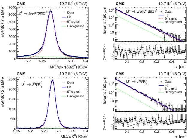
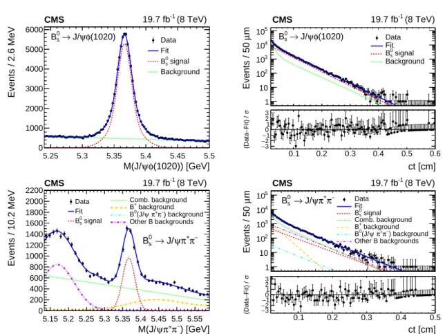
The invariant mass and ct distributions obtained from data are shown with the fit results su-perimposed in Figs. 2–4. The ct distributions are fitted in the range 0.02–0.50 cm for all modes
except the B0s → J/ψφ(1020)channel, where the upper limit is increased to 0.60 cm. The
av-erage lifetimes times the speed of light obtained from the fits are: cτB+ = 490.9±0.8 µm,
cτB0→J/ψK∗(892)0 =453.0±1.6 µm, cτB0→J/ψK0
S = 457.8±2.7 µm, cτB0s→J/ψπ+π− =502.7±10.2 µm,
cτB0
s→J/ψφ(1020) = 445.2±2.0 µm, and cτΛ0b = 442.9±8.2 µm, where all uncertainties are
statis-tical only. The B0
s →J/ψφ(1020)value given here is uncorrected for two offsets described in
Section 7. There is good agreement between the fitted functions and the data. The probabilities
5.3 Fit results 7 ct [cm] 0 0.05 0.1 0.15 0.2 0.25 0.3 0.35 0.4 0.45 0.5 Relative efficiency 0.7 0.8 0.9 1 1.1 + K ψ J/ → + B CMS Simulation ct [cm] 0 0.05 0.1 0.15 0.2 0.25 0.3 0.35 0.4 0.45 0.5 Relative efficiency 0.7 0.8 0.9 1 1.1 0 Λ ψ J/ → 0 b Λ CMS Simulation ct [cm] 0 0.05 0.1 0.15 0.2 0.25 0.3 0.35 0.4 0.45 0.5 Relative efficiency 0.7 0.8 0.9 1 1.1 0 S K ψ J/ → 0 B CMS Simulation ct [cm] 0 0.05 0.1 0.15 0.2 0.25 0.3 0.35 0.4 0.45 0.5 Relative efficiency 0.7 0.8 0.9 1 1.1 0 K*(892) ψ J/ → 0 B CMS Simulation ct [cm] 0 0.05 0.1 0.15 0.2 0.25 0.3 0.35 0.4 0.45 0.5 Relative efficiency 0.7 0.8 0.9 1 1.1 − π + π ψ J/ → 0 s B CMS Simulation ct [cm] 0 0.1 0.2 0.3 0.4 0.5 0.6 Relative efficiency 0.7 0.8 0.9 1 1.1 (1020) φ ψ J/ → s 0 B CMS Simulation
Figure 1: The combined reconstruction and selection efficiency from simulation versus ct with
a superimposed fit to an inverse power function for B+ →J/ψK+ (upper left), Λ0b →J/ψΛ0
(upper right), B0→J/ψK0S (centre left), B0→J/ψK∗(892)0 (centre right), B0s→J/ψπ+π−(lower
) [GeV] + K ψ M(J/ 5.2 5.25 5.3 5.35 5.4 Events / 2.4 MeV 0 5000 10000 15000 20000 25000 30000 Data Fit signal + B Background + K ψ J/ → + B (8 TeV) -1 19.7 fb CMS m µ Events / 50 1 10 2 10 3 10 4 10 5 10 Data Fit signal + B Background + K ψ J/ → + B ct [cm] 0.1 0.2 0.3 0.4 0.5 σ Fit) / − (Data −−32 1 −0 1 2 3 (8 TeV) -1 19.7 fb CMS ) [GeV] 0 Λ ψ M(J/ 5.45 5.5 5.55 5.6 5.65 5.7 5.75 5.8 Events / 3.5 MeV 0 50 100 150 200 250 300 350 400 Data Fit signal 0 b Λ Background 0 Λ ψ J/ → 0 b Λ (8 TeV) -1 19.7 fb CMS m µ Events / 50 1 10 2 10 3 10 Data Fit signal 0 b Λ Background 0 Λ ψ J/ → 0 b Λ ct [cm] 0.1 0.2 0.3 0.4 0.5 σ Fit) / − (Data −−32 1 −0 1 2 3 (8 TeV) -1 19.7 fb CMS
Figure 2: Invariant mass (left) and ct (right) distributions for B+ (upper) and forΛ0
b (lower)
candidates. The curves are projections of the fit to the data, with the contributions from signal (dashed), background (dotted), and the sum of signal and background (solid) shown. the lower panels of the figures on the right show the difference between the observed data and the fit divided by the data uncertainty. The vertical bars on the data points represent the statistical uncertainties.
5.3 Fit results 9 ) [GeV] 0 K*(892) ψ M(J/ 5.2 5.25 5.3 5.35 5.4 Events / 2.5 MeV 0 1000 2000 3000 4000 5000 6000 7000 Data Fit signal 0 B Background 0 K*(892) ψ J/ → 0 B (8 TeV) -1 19.7 fb CMS m µ Events / 50 1 10 2 10 3 10 4 10 Data Fit signal 0 B Background 0 K*(892) ψ J/ → 0 B ct [cm] 0.1 0.2 0.3 0.4 0.5 σ Fit) / − (Data −−32 1 −0 1 2 3 (8 TeV) -1 19.7 fb CMS ) [GeV] 0 s K ψ M(J/ 5.15 5.2 5.25 5.3 5.35 5.4 Events / 2.6 MeV 0 500 1000 1500 2000 2500 Data Fit signal 0 B Background 0 S K ψ J/ → 0 B (8 TeV) -1 19.7 fb CMS m µ Events / 50 1 10 2 10 3 10 DataFit signal 0 B Background 0 S K ψ J/ → 0 B ct [cm] 0.1 0.2 0.3 0.4 0.5 σ Fit) / − (Data −−32 1 −0 1 2 3 (8 TeV) -1 19.7 fb CMS
Figure 3: Invariant mass (left) and ct (right) distributions for B0candidates reconstructed from
J/ψK∗(892)0(upper) and J/ψK0
S(lower) decays. The curves are projections of the fit to the data,
with the contributions from signal (dashed), background (dotted), and the sum of signal and background (solid) shown. the lower panels of the figures on the right show the difference between the observed data and the fit divided by the data uncertainty. The vertical bars on the data points represent the statistical uncertainties.
(1020)) [GeV] φ ψ M(J/ 5.25 5.3 5.35 5.4 5.45 5.5 Events / 2.6 MeV 0 1000 2000 3000 4000 5000 6000 Data Fit signal s 0 B Background (8 TeV) -1 19.7 fb CMS (1020) φ ψ J/ → s 0 B mµ Events / 50 1 10 2 10 3 10 4 10 5 10 Data Fit signal s 0 B Background (1020) φ ψ J/ → s 0 B ct [cm] 0.1 0.2 0.3 0.4 0.5 0.6 σ Fit) / − (Data −−32 1 −0 1 2 3 (8 TeV) -1 19.7 fb CMS ) [GeV] − π + π ψ M(J/ 5.15 5.2 5.25 5.3 5.35 5.4 5.45 5.5 5.55 Events / 10.2 MeV 0 200 400 600 800 1000 1200 1400 1600 1800 2000 2200 Data Fit signal 0 s B Comb. background background + B ) background − π + π ψ (J/ 0 B Other B backgrounds − π + π ψ J/ → 0 s B (8 TeV) -1 19.7 fb CMS m µ Events / 50 1 10 2 10 3 10 4 10 5 10 Data Fit signal 0 s B Comb. background background + B ) background − π + π ψ (J/ 0 B Other B backgrounds − π + π ψ J/ → 0 s B ct [cm] 0.1 0.2 0.3 0.4 0.5 σ Fit) / − (Data −−32 1 −0 1 2 3 (8 TeV) -1 19.7 fb CMS
Figure 4: Invariant mass (left) and ct (right) distributions for B0s candidates reconstructed
from J/ψφ(1020) (upper) and J/ψπ+π− (lower) decays. The curves are projections of the fit
to the data, with the full fit function (solid) and signal (dashed) shown for both decays, the total background (dotted) shown for the upper plots, and the combinatorial background
(dot-ted), misidentified B+ → J/ψK+ background (dashed-dotted), B0 → J/ψπ+
π− contribution
(dashed-dotted-dotted-dotted), and partially reconstructed and other misidentified B back-grounds (dashed-dotted-dotted) shown for the lower plots. the lower panels of the figures on the right show the difference between the observed data and the fit divided by the data uncertainty. The vertical bars on the data points represent the statistical uncertainties.
11
6
Measurement of the B
+clifetime
The decay time distribution for the signal NB(ct) can be expressed as the product of an
effi-ciency function εB(ct)and an exponential decay function EB(ct) = exp(−ct/cτB), convolved
with the time resolution function of the detector r(ct). The ratio of B+c to B+events at a given
proper time can be expressed as NB+
c (ct)
NB+(ct)
≡R(ct) = εB+c(ct)[r(ct) ⊗EB+c(ct)]
εB+(ct)[r(ct) ⊗EB+(ct)]. (8)
We have verified through studies of simulated pseudo-events that Eq. (8) is not significantly affected by the time resolution, and therefore this equation can be simplified to
R(ct) ≈ Rε(ct)exp(−∆Γt), (9)
where the small effect from the time resolution is evaluated from MC simulations and is
in-cluded in Rε(ct), which denotes the ratio of the B+c and B+efficiency functions. The quantity
∆Γ is defined as ∆Γ≡ ΓB+ c −ΓB+ = 1 τB+ c − 1 τB+. (10)
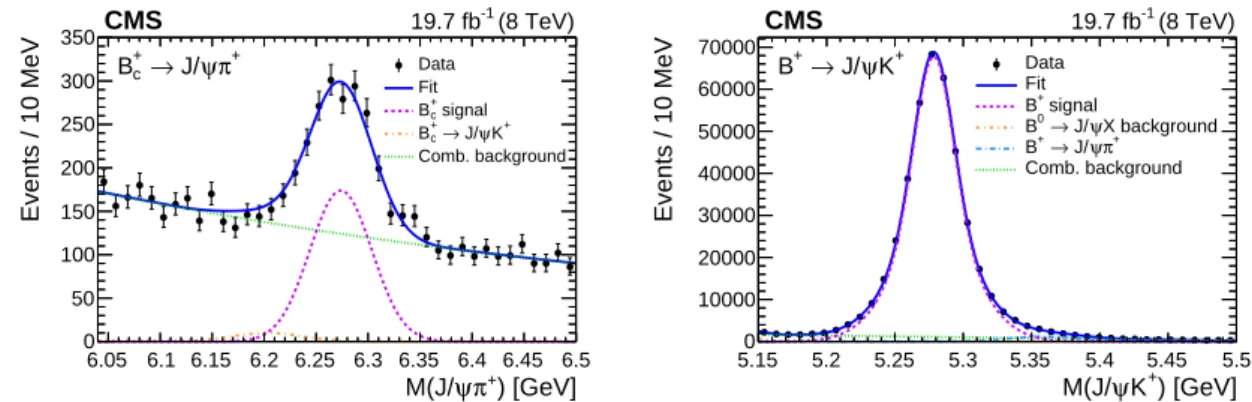
The B+c →J/ψπ+ and B+→J/ψK+invariant mass distributions, shown in Fig. 5, are each fit
with an unbinned maximum-likelihood estimator. The J/ψπ+invariant mass distribution is
fit-ted with a Gaussian function for the B+c signal and an exponential function for the background.
An additional background contribution from Bc+→J/ψK+decays is modelled from a simulated
sample of Bc+→J/ψK+events, and its contribution is constrained using the value of the
branch-ing fraction relative to J/ψπ+[27]. The B+c →J/ψπ+signal yield is 1128±60 events, where the
uncertainty is statistical only. The B+ meson invariant mass distribution is fit with a sum of
two Gaussian functions with a common mean for the signal and a second-order Chebyshev
polynomial for the background. Additional contributions from partially reconstructed B0 and
B+meson decays are parametrized with functions determined from B+→J/ψπ+and inclusive
B0→J/ψX MC samples. ) [GeV] + π ψ M(J/ 6.05 6.1 6.15 6.2 6.25 6.3 6.35 6.4 6.45 6.5 Events / 10 MeV 0 50 100 150 200 250 300 350CMS (8 TeV) -1 19.7 fb Data Fit signal + c B + K ψ J/ → + c B Comb. background + π ψ J/ → c + B ) [GeV] + K ψ M(J/ 5.15 5.2 5.25 5.3 5.35 5.4 5.45 5.5 Events / 10 MeV 0 10000 20000 30000 40000 50000 60000 70000 CMS 19.7 fb-1 (8 TeV) Data Fit signal + B X background ψ J/ → 0 B + π ψ J/ → + B Comb. background + K ψ J/ → + B
Figure 5: The J/ψπ+invariant mass distribution (left) with the solid line representing the total
fit, the dashed line the signal component, the dotted line the combinatorial background, and
the dashed-dotted line the contribution from B+
c →J/ψK+decays. The J/ψK+ invariant mass
distribution (right) with the solid line representing the total fit, the dashed line the signal
com-ponent, the dotted-dashed curves the B+→J/ψπ+and B0contributions, and the dotted curve
the combinatorial background. The vertical bars on the data points represent the statistical uncertainties.
similar statistical uncertainty in the B+
c signal yield among the bins. The bin edges are defined
by requiring a relative statistical uncertainty of 12% or better in each bin. The same binning is
used for the B+ ct distribution. The B+c and B+ meson yields are shown versus ct in the left
plot of Fig. 6, where the number of signal events is normalized by the bin width. Efficiencies are obtained from the MC samples and are defined as the ct distribution of the selected events after reconstruction divided by the ct distribution obtained from an exponential decay with the lifetime set to the same value used to generate each MC sample. The ratio of the two efficiency distributions, using the same binning scheme as for the data, is shown in the right plot of Fig. 6.
ct [cm] 0.02 0.04 0.06 0.08 0.1 ] -1 dN/d(ct) [cm 3 10 4 10 5 10 6 10 7 10 8 10 ct [cm] 0.02 0.04 0.06 0.08 0.1 ] -1 dN/d(ct) [cm 3 10 4 10 5 10 6 10 7 10 8 10 + K ψ J/ → + B + π ψ J/ → + c B CMS 19.7 fb-1 (8 TeV) ct [cm] 0.02 0.04 0.06 0.08 0.1 ε R 0.7 0.75 0.8 0.85 0.9 0.95 1CMS Simulation
Figure 6: Yields of B+c →J/ψπ+and B+→J/ψK+events (left) as a function of ct, normalized to
the bin width, as determined from fits to the invariant mass distributions. Ratio of the B+c and
B+efficiency distributions (right) as a function of ct, as determined from simulated events. The
vertical bars on the data points represent the statistical uncertainties, and the horizontal bars show the bin widths.
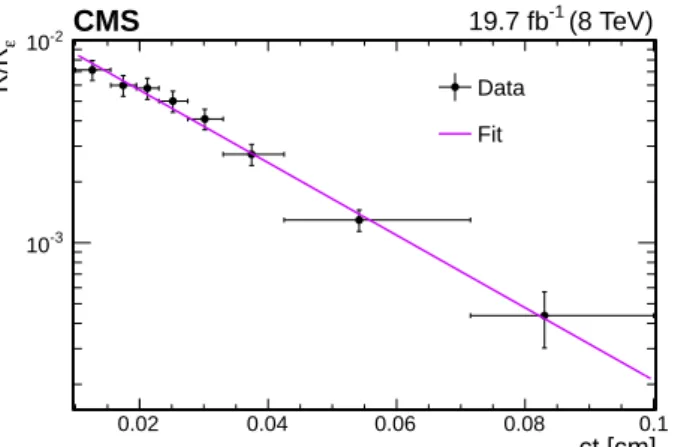
The ratio of the Bc+to B+ efficiency-corrected ct distributions, R/Rε, is shown in Fig. 7, along
with the result of a fit to an exponential function. The fit returns∆Γ=1.24±0.09 ps−1. Using
the known lifetime of the B+meson, cτB+ = 491.1±1.2 µm [5], a measurement of the B+c meson
lifetime, cτB+
c = 162.3±7.8 µm, is extracted, where the uncertainty is statistical only.
7
Systematic uncertainties
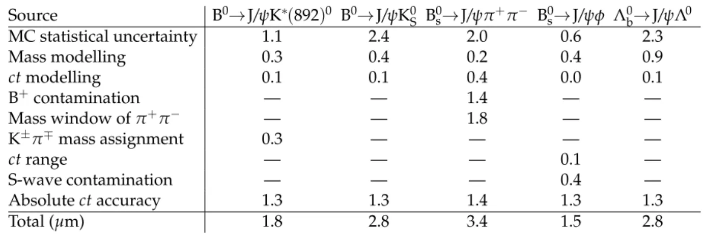
The systematic uncertainties can be divided into uncertainties common to all the measure-ments, and uncertainties specific to a decay channel. Table 1 summarizes the systematic
un-certainties for the sources considered below and the total systematic uncertainty in the B0s, B0,
andΛ0blifetime measurements. The systematic uncertainties in∆Γ and the B+c meson lifetime
are collected in Table 2. Using the known lifetime of the B+meson, the uncertainties in∆Γ are
converted into uncertainties in the B+c meson lifetime measurement. The uncertainty in the B+c
meson lifetime due to the uncertainty in the B+meson lifetime [5] is quoted separately.
We have verified that the results are stable against changes in the selection requirements on the quality of the tracks and vertices, the kinematic variables, and ct, as well as in detector regions
7.1 Common systematic uncertainties 13 ct [cm] 0.02 0.04 0.06 0.08 0.1 ε R/R -3 10 -2 10 Data Fit CMS 19.7 fb-1 (8 TeV)
Figure 7: Ratio of the B+c to B+efficiency-corrected ct distributions, R/Rε, with a line showing
the result of the fit to an exponential function. The vertical bars give the statistical uncertainty in the data, and the horizontal bars show the bin widths.
and data-taking periods. The effect of replacing the mass of the b hadron in the ct definition of Eq. (1) from the world-average to the reconstructed candidate mass is found to be negligible. The lifetimes for all decay channels were measured by treating MC samples as data. No bias was found and all results were consistent with the input lifetimes of the generated samples.
7.1 Common systematic uncertainties
1. Statistical uncertainty in the MC samples
The number of events in the simulation directly affects the accuracy of the efficiency
de-termination. In the case of the B0
s, B0, and Λ0b lifetime measurements, 1000 efficiency
curves are generated with variations of the parameter values. The parameter values are sampled using a multivariate Gaussian PDF that is constructed from the covariance ma-trix of the efficiency fit. The analysis is performed 1000 times, varying the parameters of the efficiency function. The distribution of the measured lifetimes is fitted with a Gaus-sian function, whose width is taken as the systematic uncertainty associated with the
fi-nite size of the simulated samples. In the measurement of the B+c lifetime, the bin-by-bin
statistical uncertainty in the efficiency determination is propagated to the R(ct)
distribu-tion, the fit is performed, and the difference in quadrature of the uncertainty in∆Γ with
respect to the nominal value is taken as the systematic uncertainty. 2. Modelling of the mass distribution shape
Biases related to the modelling of the shapes of the b hadron mass signal and background PDFs are quantified by changing the signal and background PDFs individually and using
the new models to fit the data. For the B0, B0
s, andΛ0blifetime measurements, the
back-ground model is changed to a higher-degree polynomial, a Chebyshev polynomial, or an exponential function, and the signal model is changed from two Gaussian functions to a single Gaussian function or a sum of three Gaussian functions. Differences in the measured lifetime between the results of the nominal and alternative models are used to estimate the systematic uncertainty, with the variations due to the modelling of signal
and background components evaluated separately and added in quadrature. For the B+c
lifetime measurement, the signal peak is alternatively modelled with a Crystal Ball dis-tribution [28]. The alternative description for the background is a first-order Chebyshev
distribution. The removal of the Cabibbo-suppressed B+
c →J/ψK+ contribution is also
considered. The maximum deviation of the signal yield in each ct bin from the nominal
that obtained with the nominal fit model. The difference between the results of the nom-inal and alternative fit models is used as the systematic uncertainty from the ct shape modelling.
2. The B+contamination in the B0s→J/ψπ+π−sample
In the nominal fit, the yield and lifetime of the B+ → J/ψK+ contamination are
deter-mined from the fit with the mass shape obtained from simulation. An alternative
esti-mate of the J/ψK+contamination is obtained from data by taking the leading pion of the
B0s→J/ψπ+π− decay to be the kaon. The lifetime and yield of the B+→J/ψK+ decays
contaminating the B0
s→J/ψπ+π−sample are determined from a fit of the B+signal
can-didates in the B0
s→J/ψπ+π− sample, with the mass shape also obtained from the data.
The difference between the B0s lifetime found with this model and the nominal model is
considered as the systematic uncertainty due to B+contamination.
3. Invariant mass window of the π+π−in the B0s→J/ψπ+π−channel
Although the events selected by the π+π− mass window are dominated by the f0(980),
its width is not well known and possible backgrounds under the f0(980)peak could be
increased or decreased, depending on the mass window. The effect on the lifetime is
studied by using mass windows of±30 and±80 MeV around the signal peak, compared
to the nominal fit result with a±50 MeV window. The maximum variation of the lifetime
is taken as the systematic uncertainty.
4. The K+π−mass assignments for K∗(892)0candidates in the B0→J/ψK∗(892)0channel
The K∗(892)0candidates are constructed from a pair of tracks with kaon and pion mass
assignments. The combination with invariant mass closest to the world-average K∗(892)0
mass is chosen to reconstruct the B0candidate. To estimate the effect on the lifetime due
to a possible misassignment of kaon and pion, both combinations are discarded if both
are within the natural width of the K∗(892)0mass, and the difference between the lifetime
obtained with this sample and the nominal sample is taken as the systematic uncertainty.
5. The ct range in the B0
s→J/ψφ(1020)channel
Since the ct > 0.02 cm requirement distorts the fractions of heavy and light mass
eigen-states, the measured B0seffective lifetime must be corrected. The correction and systematic
uncertainty are quantified analytically. The correction to the effective lifetime is
δct =cτeffcut−cτeff =
(1− |A⊥|2)(cτL)2e−a/cτL + |A⊥|2(cτH)2e−a/cτH (1− |A⊥|2)cτLe−a/cτL + |A⊥|2cτHe−a/cτH −(1− |A⊥| 2)(cτ L)2+ |A⊥|2(cτH)2 (1− |A⊥|2)cτL+ |A⊥|2cτH , (11)
where the first term represents the effective lifetime in the presence of a ct > a
require-ment and the latter term is the unbiased effective lifetime. In this analysis, a is equal to
0.02 cm. The world-average values [2] for cτH = 482.7±3.6 µm, cτL = 426.3±2.4 µm,
7.2 Channel-specific systematic uncertainties 15
6. The S-wave contamination in the B0s→J/ψφ(1020)channel
The B0s candidates reconstructed in the J/ψφ(1020)final state contain a small fraction of
nonresonant and CP-odd B0s →J/ψK+K− decays, where the invariant mass of the two
kaons happens to be near the φ meson mass. The fraction of B0
s → J/ψK+K− decays
among the selected events is measured in the weak mixing phase analysis [9] to be fS =
(1.2+−0.90.7)%. Because of the different trigger and signal selection criteria of the present
analysis, the S-wave fraction is corrected according to the simulation to be (1.5+−1.10.9)%.
The bias caused by the contamination of nonresonant B0s→J/ψK+K−decays is estimated
by generating two sets of pseudo-experiments, one with just B0s → J/ψφ(1020) events
and one with a fraction of S-wave events based on the measured S-wave fraction and its uncertainty. The difference in the average of the measured lifetimes of these two samples is 0.74 µm, which is used to correct the measured lifetime. The systematic uncertainty associated with this correction is obtained by taking the difference in quadrature between the standard deviation of the distribution of lifetime results from the pseudo-experiments with and without the S-wave contribution.
7. PV selection in the B+c →J/ψπ+channel
From the multiple reconstructed PVs in an event, one is selected to compute the ct value of the candidate. Two alternative methods to select the PV position are studied: using
the centre of the beamspot and selecting the PV with the largest sum of track pT. While
all three methods are found to be effective and unbiased, there were small differences, and the maximum deviation with respect to the nominal choice is taken as the systematic
uncertainty. The B+and B+c primary vertex choices were changed coherently.
8. Detector alignment in the Bc+→J/ψπ+channel
Possible effects on the lifetime due to uncertainties in the detector alignment [29] are in-vestigated for each decay topology using 20 different simulated samples with distorted geometries. These distortions include expansions in the radial and longitudinal dimen-sions, rotations, twists, offsets, etc. The amount of misalignment is chosen such that it is large enough to be detected and corrected by the alignment procedure. The standard deviation of the lifetimes for the tested scenarios is taken as the systematic uncertainty
from this source. The B+and B+c geometries were changed coherently.
9. Absolute ct accuracy in the B0s, B0, andΛ0blifetime measurements
The lifetime of the most statistically precise mode (B+→J/ψK+) is used to validate the
accuracy of the simulation and various detector calibrations. The difference between our
measurement of 490.9±0.8 µm (statistical uncertainty only) and the world-average value
of 491.1±1.2 µm [5] is 0.2±1.4 µm. This implies a limit to the validation of 1.4/491 =
0.3%. Four systematic effects that we expect to be included were checked independently. The systematic uncertainties from PV selection and detector alignment were found to be 0.7 µm and 0.3–0.7 µm, respectively. Varying the efficiency functional form changed the
lifetimes by 0.3–0.6 µm, while varying σct by factors of 0.5 and 2.0 resulted in lifetime
differences of no more than 0.2 µm. As the sum in quadrature of these uncertainties is
less than that obtained from the B+lifetime comparison, we assign a value of 0.3% as the
B contamination — — 1.4 — — Mass window of π+π− — — 1.8 — — K±π∓mass assignment 0.3 — — — — ct range — — — 0.1 — S-wave contamination — — — 0.4 — Absolute ct accuracy 1.3 1.3 1.4 1.3 1.3 Total (µm) 1.8 2.8 3.4 1.5 2.8
Table 2: Summary of the systematic uncertainties in the∆Γ and cτB+
c measurements. Source ∆Γ [ps−1] cτB+ c [µm] MC statistical uncertainty 0.01 1.2 Mass modelling 0.04 3.4 PV selection 0.02 2.0 Detector alignment 0.01 0.6 Total uncertainty 0.05 4.2
8
Lifetime measurement results
Our final results for the B0, B0
s, andΛ0bhadron lifetimes are:
cτB0→J/ψK∗(892)0 =453.0±1.6 (stat)±1.8 (syst) µm, (12) cτB0→J/ψK0 S=457.8±2.7 (stat)±2.8 (syst) µm, (13) cτB0 s→J/ψπ+π− =502.7±10.2 (stat)±3.4 (syst) µm, (14) cτB0 s→J/ψφ(1020)=443.9±2.0 (stat)±1.5 (syst) µm, (15) cτΛ0 b =442.9±8.2 (stat)±2.8 (syst) µm. (16)
The value of the B0
s lifetime using the J/ψφ(1020)decay has been corrected for the ct range and
S-wave contamination effects described in Section 7. The lifetime ratios τB0
s/τB0 and τΛ0b/τB0
have been determined using the decay channels B0→J/ψK∗(892)0, Bs0→J/ψφ(1020), andΛ0b→
J/ψΛ0. Including the statistical and correlated and uncorrelated systematic uncertainties, the
results are:
τΛ0
b/τB0→J/ψK∗(892)0 =0.978±0.018 (stat)±0.006 (syst), (17)
τB0
s→J/ψφ(1020)/τB0→J/ψK∗(892)0 =0.980±0.006 (stat)±0.003 (syst). (18)
These ratios are compatible with the current world-average values.
The measured lifetimes for the B0meson in the two different channels are in agreement.
Com-bining the two results, including the statistical and the correlated and uncorrelated systematic
uncertainties, gives cτB0 = 454.1±1.4 (stat)±1.7 (syst) µm. The lifetime measurements can
17
two B0decay modes can be written as:
τB0→J/ψK0 S = 1 Γd 1 1−y2 d ! 1+2 cos(2β)yd+y2d 1+cos(2β)yd ! , (19) τB0→J/ψK∗(892)0 = 1 Γd 1+y2d 1−y2 d ! , (20)
where yd = ∆Γd/2Γd, and β = (21.9±0.7)◦ [5] is one of the CKM unitarity triangle angles.
Using our measured values for the two B0 lifetimes, we fit forΓd and∆Γd and use the values
to determine∆Γd/Γd. The results are:
Γd =0.662±0.003 (stat)±0.003 (syst) ps−1, (21)
∆Γd =0.023±0.015 (stat)±0.016 (syst) ps−1, (22)
∆Γd/Γd =0.034±0.023 (stat)±0.024 (syst). (23)
Neglecting CP violation in mixing, the measured B0s→J/ψπ+π−lifetime can be translated into
the width of the heavy B0
s mass eigenstate:
ΓH=1/τB0
s =0.596±0.012 (stat)±0.004 (syst) ps
−1. (24)
Solving for cτLfrom Eq. (4) gives
cτL = 1 2cτeff+ s 1 4(cτeff) 2− |A⊥|2 1− |A⊥|2 cτH(cτH−cτeff). (25)
Using the B0s → J/ψπ+π− result in Eq. (14), the measured B0s effective lifetime in Eq. (15),
and the world-average value of the magnitude squared of the CP-odd amplitude |A⊥|2 =
0.250±0.006 [2], the lifetime of the light component is found to be cτL = 420.4±6.2 µm. The
uncertainty includes all statistical and systematic uncertainties, taking into account the
corre-lated uncertainties. The result is consistent with the world-average value of 423.6±1.8 µm [5].
Our measured lifetimes for B0, B0
s → J/ψφ(1020), and Λ0b are compatible with the current
world-average values [5] of 455.7±1.2 µm, 443.4±3.6 µm, and 440.7±3.0 µm, respectively.
In addition, our measurement of the B0s lifetime in the B0s→J/ψπ+π−channel is in agreement
with the results from CDF, LHCb, and D0: 510+−3633(stat)±9 (syst) µm [30], 495.3±7.2 (stat)±
7.2 (syst) µm [31], and 508±42 (stat)±16 (syst) µm [32], respectively.
Our final result for the Bc+lifetime using the J/ψπ+mode is:
cτB+
c =162.3±7.8 (stat)±4.2 (syst)±0.1(τB+)µm, (26)
where the systematic uncertainty from the B+ lifetime uncertainty [5] is quoted separately in
the result. This measurement is in agreement with the world-average value(152.0±2.7 µm)[5].
Precise measurements of the Bc+lifetime allow tests of various theoretical models, which
pre-dict values ranging from 90 to 210 µm [33–36]. Furthermore, they provide new constraints
on possible physics beyond the standard model from the observed anomalies in B → D(∗)τν
results are used to obtain an average lifetime and to measure the decay width difference
be-tween the two mass eigenstates. The B0s lifetime results are used to obtain the lifetimes of the
heavy and light B0s mass eigenstates. The precision of theΛ0blifetime measurement is also as
good as any previous measurement in the J/ψΛ0channel. The measured B+
c meson lifetime is
in agreement with the results from LHCb and significantly more precise than the CDF and D0 measurements. All measured lifetimes are compatible with the current world-average values.
Acknowledgments
We congratulate our colleagues in the CERN accelerator departments for the excellent perfor-mance of the LHC and thank the technical and administrative staffs at CERN and at other CMS institutes for their contributions to the success of the CMS effort. In addition, we grate-fully acknowledge the computing centres and personnel of the Worldwide LHC Computing Grid for delivering so effectively the computing infrastructure essential to our analyses. Fi-nally, we acknowledge the enduring support for the construction and operation of the LHC and the CMS detector provided by the following funding agencies: BMWFW and FWF (Aus-tria); FNRS and FWO (Belgium); CNPq, CAPES, FAPERJ, and FAPESP (Brazil); MES (Bulgaria); CERN; CAS, MoST, and NSFC (China); COLCIENCIAS (Colombia); MSES and CSF (Croatia); RPF (Cyprus); SENESCYT (Ecuador); MoER, ERC IUT, and ERDF (Estonia); Academy of Fin-land, MEC, and HIP (Finland); CEA and CNRS/IN2P3 (France); BMBF, DFG, and HGF (Ger-many); GSRT (Greece); OTKA and NIH (Hungary); DAE and DST (India); IPM (Iran); SFI (Ireland); INFN (Italy); MSIP and NRF (Republic of Korea); LAS (Lithuania); MOE and UM (Malaysia); BUAP, CINVESTAV, CONACYT, LNS, SEP, and UASLP-FAI (Mexico); MBIE (New Zealand); PAEC (Pakistan); MSHE and NSC (Poland); FCT (Portugal); JINR (Dubna); MON, RosAtom, RAS, RFBR and RAEP (Russia); MESTD (Serbia); SEIDI, CPAN, PCTI and FEDER (Spain); Swiss Funding Agencies (Switzerland); MST (Taipei); ThEPCenter, IPST, STAR, and NSTDA (Thailand); TUBITAK and TAEK (Turkey); NASU and SFFR (Ukraine); STFC (United Kingdom); DOE and NSF (USA).
Individuals have received support from the Marie-Curie programme and the European Re-search Council and Horizon 2020 Grant, contract No. 675440 (European Union); the Lev-entis Foundation; the A. P. Sloan Foundation; the Alexander von Humboldt Foundation; the Belgian Federal Science Policy Office; the Fonds pour la Formation `a la Recherche dans l’Industrie et dans l’Agriculture (FRIA-Belgium); the Agentschap voor Innovatie door Weten-schap en Technologie (IWT-Belgium); the Ministry of Education, Youth and Sports (MEYS) of the Czech Republic; the Council of Science and Industrial Research, India; the HOMING PLUS program of the Foundation for Polish Science, cofinanced from European Union, Re-gional Development Fund, the Mobility Plus program of the Ministry of Science and Higher Education, the National Science Center (Poland), contracts Harmonia 2014/14/M/ST2/00428, Opus 2014/13/B/ST2/02543, 2014/15/B/ST2/03998, and 2015/19/B/ST2/02861, Sonata-bis 2012/07/E/ST2/01406; the National Priorities Research Program by Qatar National Research Fund; the Programa Severo Ochoa del Principado de Asturias; the Thalis and Aristeia programs
References 19
cofinanced by EU-ESF and the Greek NSRF; the Rachadapisek Sompot Fund for Postdoctoral Fellowship, Chulalongkorn University and the Chulalongkorn Academic into Its 2nd Century Project Advancement Project (Thailand); the Welch Foundation, contract C-1845; and the We-ston Havens Foundation (USA).
References
[1] A. Lenz, “Lifetimes and heavy quark expansion”, Int. J. Mod. Phys. A 30 (2015) 1543005, doi:10.1142/S0217751X15430058.
[2] Particle Data Group, C. Patrignani et al., “Review of particle physics”, Chin. Phys. C 40 (2016) 100001, doi:10.1088/1674-1137/40/10/100001.
[3] CMS Collaboration, “The CMS experiment at the CERN LHC”, JINST 3 (2008) S08004, doi:10.1088/1748-0221/3/08/S08004.
[4] R. Fleischer and R. Knegjens, “Effective lifetimes of Bsdecays and their constraints on the
B0s–B0s mixing parameters”, Eur. Phys. J. C 71 (2011) 1789,
doi:10.1140/epjc/s10052-011-1789-9, arXiv:1109.5115.
[5] Heavy Flavor Averaging Group, Y. Amhis et al., “Averages of b-hadron, c-hadron, and
τ-lepton properties as of summer 2016”, Eur. Phys. J. C 77 (2017) 895,
doi:10.1140/epjc/s10052-017-5058-4, arXiv:1612.07233.
[6] T. Gershon, “∆Γd: a forgotten null test of the standard model”, J. Phys. G 38 (2011)
doi:10.1088/0954-3899/38/1/015007, arXiv:1007.5135.
[7] LHCb Collaboration, “Analysis of the resonant components in B0
s → J/ψπ+π−”, Phys.
Rev. D 86 (2012) 052006, doi:10.1103/PhysRevD.86.052006, arXiv:1301.5347. [8] LHCb Collaboration, “Measurement of resonant and CP components in
B0s → J/ψπ+π−”, Phys. Rev. D 89 (2014) 092006,
doi:10.1103/PhysRevD.89.092006, arXiv:1402.6248.
[9] CMS Collaboration, “Measurement of the CP-violating weak phase φsand the decay
width difference∆Γsusing the B0s → J/ψφ(1020) decay channel in pp collisions at
√
s=
8 TeV”, Phys. Lett. B 757 (2016) 97, doi:10.1016/j.physletb.2016.03.046, arXiv:1507.07527.
[10] V. V. Kiselev, “Exclusive decays and lifetime of Bcmeson in QCD sum rules”, (2002).
arXiv:hep-ph/0211021.
[11] LHCb Collaboration, “Measurement of the B+
c meson lifetime using B+c → J/ψµ+νµX
decays”, Eur. Phys. J. C 74 (2014) 2839, doi:10.1140/epjc/s10052-014-2839-x,
arXiv:1401.6932.
[12] LHCb Collaboration, “Measurement of the lifetime of the B+c meson using the
B+
c → J/ψπ+decay mode”, Phys. Lett. B 742 (2015) 29,
doi:10.1016/j.physletb.2015.01.010, arXiv:1411.6899.
[13] CDF Collaboration, “Observation of the Bcmeson in pp collisions at
√
s=1.8 TeV”, Phys.
Rev. Lett. 81 (1998) 2432, doi:10.1103/PhysRevLett.81.2432, arXiv:hep-ex/9805034.
[16] CDF Collaboration, “Measurement of the Bc meson lifetime in the decay Bc → J/ψπ ”, Phys. Rev. D 87 (2013) 011101, doi:10.1103/PhysRevD.87.011101,
arXiv:1210.2366.
[17] CMS Collaboration, “Description and performance of track and primary-vertex reconstruction with the CMS tracker”, JINST 9 (2014) P10009,
doi:10.1088/1748-0221/9/10/P10009, arXiv:1405.6569.
[18] CMS Collaboration, “The CMS trigger system”, JINST 12 (2017) P01020, doi:10.1088/1748-0221/12/01/P01020, arXiv:1609.02366.
[19] T. Sj ¨ostrand, S. Mrenna, and P. Z. Skands, “PYTHIA 6.4 physics and manual”, JHEP 05 (2006) 026, doi:10.1088/1126-6708/2006/05/026, arXiv:hep-ph/0603175. [20] C. Chang, C. Driouchi, P. Eerola, and X. Wu, “BCVEGPY: an event generator for hadronic
production of the Bc meson”, Comput. Phys. Commun. 159 (2004) 192,
doi:10.1016/j.cpc.2004.02.005, arXiv:hep-ph/0309120.
[21] C. Chang, J. Wang, and X. Wu, “BCVEGPY2.0: An upgraded version of the generator
BCVEGPY with the addition of hadroproduction of the P-wave Bcstates”, Comput. Phys.
Commun. 174 (2006) 241, doi:10.1016/j.cpc.2005.09.008,
arXiv:hep-ph/0504017.
[22] D. J. Lange, “The EvtGen particle decay simulation package”, Nucl. Instrum. Meth. A 462 (2001) 152, doi:10.1016/S0168-9002(01)00089-4.
[23] P. Golonka and Z. Wa¸s, “PHOTOS Monte Carlo: a precision tool for QED corrections in Z and W decays”, Eur. Phys. J. C 45 (2006) 97, doi:10.1140/epjc/s2005-02396-4, arXiv:hep-ph/0506026.
[24] GEANT4 Collaboration, “GEANT4—a simulation toolkit”, Nucl. Instrum. Meth. A 506 (2003) 250, doi:10.1016/S0168-9002(03)01368-8.
[25] CMS Collaboration, “Performance of CMS muon reconstruction in pp collision events at√
s =7 TeV”, JINST 7 (2012) P10002, doi:10.1088/1748-0221/7/10/P10002,
arXiv:1206.4071.
[26] A. S. Dighe, I. Dunietz, and R. Fleischer, “Extracting CKM phases and Bs−Bsmixing
parameters from angular distributions of non-leptonic B decays”, Eur. Phys. J. C 6 (1999) 647, doi:10.1007/s100529800954, arXiv:hep-ph/9804253.
[27] LHCb Collaboration, “First observation of the decay B+c →J/ψ K+”, JHEP 09 (2013) 075,
doi:10.1007/JHEP09(2013)075, arXiv:1306.6723.
[28] M. J. Oreglia, “A study of the reactions ψ0 →γγψ”. PhD thesis, Stanford University,
References 21
[29] CMS Collaboration, “Alignment of the CMS tracker with LHC and cosmic ray data”, JINST 9 (2014) P06009, doi:10.1088/1748-0221/9/06/P06009,
arXiv:1403.2286.
[30] CDF Collaboration, “Measurement of branching ratio and B0s lifetime in the decay
B0s → J/ψf0(980)at CDF”, Phys. Rev. D 84 (2011) 052012,
doi:10.1103/PhysRevD.84.052012, arXiv:1106.3682.
[31] LHCb Collaboration, “Measurement of CP violation and the B0s meson decay width
difference with B0s → J/ψK+K−and B0s → J/ψπ+π−decays”, Phys. Rev. D 87 (2013)
112010, doi:10.1103/PhysRevD.87.112010, arXiv:1304.2600.
[32] D0 Collaboration, “B0
s lifetime measurement in the CP-odd decay channel
B0s → J/ψf0(980)”, Phys. Rev. D 94 (2016) 012001,
doi:10.1103/PhysRevD.94.012001, arXiv:1603.01302.
[33] C.-H. Chang, S.-L. Chen, T.-F. Feng, and X.-Q. Li, “Lifetime of the Bcmeson and some
relevant problems”, Phys. Rev. D 64 (2001) 014003,
doi:10.1103/PhysRevD.64.014003, arXiv:hep-ph/0007162.
[34] M. Beneke and G. Buchalla, “Bcmeson lifetime”, Phys. Rev. D 53 (1996) 4991,
doi:10.1103/PhysRevD.53.4991, arXiv:hep-ph/9601249.
[35] A. Yu. Anisimov, I. M. Narodetskii, C. Semay, and B. Silvestre-Brac, “The Bcmeson
lifetime in the light-front constituent quark model”, Phys. Lett. B 452 (1999) 129,
doi:10.1016/S0370-2693(99)00273-7, arXiv:hep-ph/9812514.
[36] V. V. Kiselev, A. E. Kovalsky, and A. K. Likhoded, “Decays and lifetime of Bcin QCD sum
rules”, in 5th International Workshop on Heavy Quark Physics, Dubna, Russia, April 6-8, 2000. arXiv:hep-ph/0006104.
[37] R. Alonso, B. Grinstein, and J. Martin Camalich, “Lifetime of B−c constrains explanations
for anomalies in B→D(∗)τν”, Phys. Rev. Lett. 118 (2017) 081802,
23
A
The CMS Collaboration
Yerevan Physics Institute, Yerevan, Armenia A.M. Sirunyan, A. Tumasyan
Institut f ¨ur Hochenergiephysik, Wien, Austria
W. Adam, F. Ambrogi, E. Asilar, T. Bergauer, J. Brandstetter, E. Brondolin, M. Dragicevic, J. Er ¨o,
M. Flechl, M. Friedl, R. Fr ¨uhwirth1, V.M. Ghete, J. Grossmann, J. Hrubec, M. Jeitler1, A. K ¨onig,
N. Krammer, I. Kr¨atschmer, D. Liko, T. Madlener, I. Mikulec, E. Pree, N. Rad, H. Rohringer,
J. Schieck1, R. Sch ¨ofbeck, M. Spanring, D. Spitzbart, W. Waltenberger, J. Wittmann, C.-E. Wulz1,
M. Zarucki
Institute for Nuclear Problems, Minsk, Belarus Y. Dydyshka, V. Mossolov, J. Suarez Gonzalez Universiteit Antwerpen, Antwerpen, Belgium
E.A. De Wolf, D. Di Croce, X. Janssen, J. Lauwers, H. Van Haevermaet, P. Van Mechelen, N. Van Remortel
Vrije Universiteit Brussel, Brussel, Belgium
S. Abu Zeid, F. Blekman, J. D’Hondt, I. De Bruyn, J. De Clercq, K. Deroover, G. Flouris, D. Lontkovskyi, S. Lowette, S. Moortgat, L. Moreels, Q. Python, K. Skovpen, S. Tavernier, W. Van Doninck, P. Van Mulders, I. Van Parijs
Universit´e Libre de Bruxelles, Bruxelles, Belgium
D. Beghin, H. Brun, B. Clerbaux, G. De Lentdecker, H. Delannoy, B. Dorney, G. Fasanella, L. Favart, R. Goldouzian, A. Grebenyuk, G. Karapostoli, T. Lenzi, J. Luetic, T. Maerschalk, A. Marinov, A. Randle-conde, T. Seva, C. Vander Velde, P. Vanlaer, D. Vannerom, R. Yonamine,
F. Zenoni, F. Zhang2
Ghent University, Ghent, Belgium
A. Cimmino, T. Cornelis, D. Dobur, A. Fagot, M. Gul, I. Khvastunov, D. Poyraz, C. Roskas, S. Salva, M. Tytgat, W. Verbeke, N. Zaganidis
Universit´e Catholique de Louvain, Louvain-la-Neuve, Belgium
H. Bakhshiansohi, O. Bondu, S. Brochet, G. Bruno, C. Caputo, A. Caudron, P. David, S. De Visscher, C. Delaere, M. Delcourt, B. Francois, A. Giammanco, M. Komm, G. Krintiras, V. Lemaitre, A. Magitteri, A. Mertens, M. Musich, K. Piotrzkowski, L. Quertenmont, A. Saggio, M. Vidal Marono, S. Wertz, J. Zobec
Universit´e de Mons, Mons, Belgium N. Beliy
Centro Brasileiro de Pesquisas Fisicas, Rio de Janeiro, Brazil
W.L. Ald´a J ´unior, F.L. Alves, G.A. Alves, L. Brito, M. Correa Martins Junior, C. Hensel, A. Moraes, M.E. Pol, P. Rebello Teles
Universidade do Estado do Rio de Janeiro, Rio de Janeiro, Brazil
E. Belchior Batista Das Chagas, W. Carvalho, J. Chinellato3, E. Coelho, E.M. Da Costa, G.G. Da
Silveira4, D. De Jesus Damiao, S. Fonseca De Souza, L.M. Huertas Guativa, H. Malbouisson,
M. Melo De Almeida, C. Mora Herrera, L. Mundim, H. Nogima, L.J. Sanchez Rosas, A. Santoro,
A. Dimitrov, I. Glushkov, L. Litov, B. Pavlov, P. Petkov Beihang University, Beijing, China
W. Fang5, X. Gao5, L. Yuan
Institute of High Energy Physics, Beijing, China
M. Ahmad, J.G. Bian, G.M. Chen, H.S. Chen, M. Chen, Y. Chen, C.H. Jiang, D. Leggat, H. Liao, Z. Liu, F. Romeo, S.M. Shaheen, A. Spiezia, J. Tao, C. Wang, Z. Wang, E. Yazgan, H. Zhang, S. Zhang, J. Zhao
State Key Laboratory of Nuclear Physics and Technology, Peking University, Beijing, China Y. Ban, G. Chen, Q. Li, S. Liu, Y. Mao, S.J. Qian, D. Wang, Z. Xu
Universidad de Los Andes, Bogota, Colombia
C. Avila, A. Cabrera, L.F. Chaparro Sierra, C. Florez, C.F. Gonz´alez Hern´andez, J.D. Ruiz Alvarez
University of Split, Faculty of Electrical Engineering, Mechanical Engineering and Naval Architecture, Split, Croatia
B. Courbon, N. Godinovic, D. Lelas, I. Puljak, P.M. Ribeiro Cipriano, T. Sculac University of Split, Faculty of Science, Split, Croatia
Z. Antunovic, M. Kovac
Institute Rudjer Boskovic, Zagreb, Croatia
V. Brigljevic, D. Ferencek, K. Kadija, B. Mesic, A. Starodumov6, T. Susa
University of Cyprus, Nicosia, Cyprus
M.W. Ather, A. Attikis, G. Mavromanolakis, J. Mousa, C. Nicolaou, F. Ptochos, P.A. Razis, H. Rykaczewski
Charles University, Prague, Czech Republic
M. Finger7, M. Finger Jr.7
Universidad San Francisco de Quito, Quito, Ecuador E. Carrera Jarrin
Academy of Scientific Research and Technology of the Arab Republic of Egypt, Egyptian Network of High Energy Physics, Cairo, Egypt
Y. Assran8,9, S. Elgammal9, A. Mahrous10
National Institute of Chemical Physics and Biophysics, Tallinn, Estonia R.K. Dewanjee, M. Kadastik, L. Perrini, M. Raidal, A. Tiko, C. Veelken Department of Physics, University of Helsinki, Helsinki, Finland P. Eerola, H. Kirschenmann, J. Pekkanen, M. Voutilainen
25
Helsinki Institute of Physics, Helsinki, Finland
T. J¨arvinen, V. Karim¨aki, R. Kinnunen, T. Lamp´en, K. Lassila-Perini, S. Lehti, T. Lind´en, P. Luukka, E. Tuominen, J. Tuominiemi
Lappeenranta University of Technology, Lappeenranta, Finland J. Talvitie, T. Tuuva
IRFU, CEA, Universit´e Paris-Saclay, Gif-sur-Yvette, France
M. Besancon, F. Couderc, M. Dejardin, D. Denegri, J.L. Faure, F. Ferri, S. Ganjour, S. Ghosh, A. Givernaud, P. Gras, G. Hamel de Monchenault, P. Jarry, I. Kucher, C. Leloup, E. Locci,
M. Machet, J. Malcles, G. Negro, J. Rander, A. Rosowsky, M. ¨O. Sahin, M. Titov
Laboratoire Leprince-Ringuet, Ecole polytechnique, CNRS/IN2P3, Universit´e Paris-Saclay, Palaiseau, France
A. Abdulsalam, C. Amendola, I. Antropov, S. Baffioni, F. Beaudette, P. Busson, L. Cadamuro, C. Charlot, R. Granier de Cassagnac, M. Jo, S. Lisniak, A. Lobanov, J. Martin Blanco, M. Nguyen, C. Ochando, G. Ortona, P. Paganini, P. Pigard, R. Salerno, J.B. Sauvan, Y. Sirois, A.G. Stahl Leiton, T. Strebler, Y. Yilmaz, A. Zabi, A. Zghiche
Universit´e de Strasbourg, CNRS, IPHC UMR 7178, Strasbourg, France
J.-L. Agram11, J. Andrea, D. Bloch, J.-M. Brom, M. Buttignol, E.C. Chabert, N. Chanon,
C. Collard, E. Conte11, X. Coubez, J.-C. Fontaine11, D. Gel´e, U. Goerlach, M. Jansov´a, A.-C. Le
Bihan, N. Tonon, P. Van Hove
Centre de Calcul de l’Institut National de Physique Nucleaire et de Physique des Particules, CNRS/IN2P3, Villeurbanne, France
S. Gadrat
Universit´e de Lyon, Universit´e Claude Bernard Lyon 1, CNRS-IN2P3, Institut de Physique Nucl´eaire de Lyon, Villeurbanne, France
S. Beauceron, C. Bernet, G. Boudoul, R. Chierici, D. Contardo, P. Depasse, H. El Mamouni, J. Fay, L. Finco, S. Gascon, M. Gouzevitch, G. Grenier, B. Ille, F. Lagarde, I.B. Laktineh,
M. Lethuillier, L. Mirabito, A.L. Pequegnot, S. Perries, A. Popov12, V. Sordini, M. Vander
Donckt, S. Viret
Georgian Technical University, Tbilisi, Georgia T. Toriashvili13
Tbilisi State University, Tbilisi, Georgia
I. Bagaturia14
RWTH Aachen University, I. Physikalisches Institut, Aachen, Germany
C. Autermann, L. Feld, M.K. Kiesel, K. Klein, M. Lipinski, M. Preuten, C. Schomakers, J. Schulz,
T. Verlage, V. Zhukov12
RWTH Aachen University, III. Physikalisches Institut A, Aachen, Germany
A. Albert, E. Dietz-Laursonn, D. Duchardt, M. Endres, M. Erdmann, S. Erdweg, T. Esch, R. Fischer, A. G ¨uth, M. Hamer, T. Hebbeker, C. Heidemann, K. Hoepfner, S. Knutzen, M. Merschmeyer, A. Meyer, P. Millet, S. Mukherjee, T. Pook, M. Radziej, H. Reithler, M. Rieger, F. Scheuch, D. Teyssier, S. Th ¨uer
RWTH Aachen University, III. Physikalisches Institut B, Aachen, Germany
G. Fl ¨ugge, B. Kargoll, T. Kress, A. K ¨unsken, J. Lingemann, T. M ¨uller, A. Nehrkorn, A. Nowack,
J. Mnich, A. Mussgiller, E. Ntomari, D. Pitzl, A. Raspereza, B. Roland, M. Savitskyi, P. Saxena, R. Shevchenko, S. Spannagel, N. Stefaniuk, G.P. Van Onsem, R. Walsh, Y. Wen, K. Wichmann, C. Wissing, O. Zenaiev
University of Hamburg, Hamburg, Germany
R. Aggleton, S. Bein, V. Blobel, M. Centis Vignali, T. Dreyer, E. Garutti, D. Gonzalez, J. Haller, A. Hinzmann, M. Hoffmann, A. Karavdina, R. Klanner, R. Kogler, N. Kovalchuk, S. Kurz,
T. Lapsien, I. Marchesini, D. Marconi, M. Meyer, M. Niedziela, D. Nowatschin, F. Pantaleo15,
T. Peiffer, A. Perieanu, C. Scharf, P. Schleper, A. Schmidt, S. Schumann, J. Schwandt, J. Sonneveld, H. Stadie, G. Steinbr ¨uck, F.M. Stober, M. St ¨over, H. Tholen, D. Troendle, E. Usai, L. Vanelderen, A. Vanhoefer, B. Vormwald
Karlsruher Institut fuer Technology
M. Akbiyik, C. Barth, S. Baur, E. Butz, R. Caspart, T. Chwalek, F. Colombo, W. De Boer,
A. Dierlamm, B. Freund, R. Friese, M. Giffels, D. Haitz, F. Hartmann15, S.M. Heindl,
U. Husemann, F. Kassel15, S. Kudella, H. Mildner, M.U. Mozer, Th. M ¨uller, M. Plagge, G. Quast,
K. Rabbertz, M. Schr ¨oder, I. Shvetsov, G. Sieber, H.J. Simonis, R. Ulrich, S. Wayand, M. Weber, T. Weiler, S. Williamson, C. W ¨ohrmann, R. Wolf
Institute of Nuclear and Particle Physics (INPP), NCSR Demokritos, Aghia Paraskevi, Greece
G. Anagnostou, G. Daskalakis, T. Geralis, V.A. Giakoumopoulou, A. Kyriakis, D. Loukas, I. Topsis-Giotis
National and Kapodistrian University of Athens, Athens, Greece G. Karathanasis, S. Kesisoglou, A. Panagiotou, N. Saoulidou National Technical University of Athens, Athens, Greece K. Kousouris
University of Io´annina, Io´annina, Greece
I. Evangelou, C. Foudas, P. Kokkas, S. Mallios, N. Manthos, I. Papadopoulos, E. Paradas, J. Strologas, F.A. Triantis
MTA-ELTE Lend ¨ulet CMS Particle and Nuclear Physics Group, E ¨otv ¨os Lor´and University, Budapest, Hungary
M. Csanad, N. Filipovic, G. Pasztor, O. Sur´anyi, G.I. Veres19
Wigner Research Centre for Physics, Budapest, Hungary
G. Bencze, C. Hajdu, D. Horvath20, ´A. Hunyadi, F. Sikler, V. Veszpremi, A.J. Zsigmond
Institute of Nuclear Research ATOMKI, Debrecen, Hungary
N. Beni, S. Czellar, J. Karancsi21, A. Makovec, J. Molnar, Z. Szillasi
Institute of Physics, University of Debrecen, Debrecen, Hungary