Design of an Optimal Controller With Load Compensation for Transport in a Industrial Extrusion Line

Faculdade de Engenharia da Universidade do Porto

Design of an optimal controller with load

compensation for transport in an industrial

extrusion line

Bruno Filipe Ferreira Brito

Dissertation prepared under the

Master in Electrical and Computers Engineering

Major Automation

Supervisor: Prof. Dr. Adriano Silva Carvalho

Co-supervisor: Eng.º José Pedro Silva

ii

iii

“A brother may not be a friend but a friend will always be a brother” Benjamin Franklin

v

Resumo

Nos dias que correm, a competição ao nível industrial assume um carácter mundial, centrando-se na conquista de novos mercados. Este clima de competição é visível inclusivamente entre as filiais da mesma companhia uma vez que todas querem produzir mais, melhor e com menor custo. Investindo, para isso, no desenvolvimento do produto e nas suas linhas produção. Portanto, uma linha de produção é como um processo em constante mudança e evolução tecnológica, no sentido da automatização do processo, de garantir a qualidade do produto e obter o menor custo de produção. Este necessita ainda de se adaptar aos requisitos do produto.

Apesar de todas as máquinas na Continental Mabor trabalharem acima da velocidade máxima indicada pelos fabricantes ainda existem sistemas rudimentares e que começam a apresentar bastante imprecisão para as velocidades elevadas de trabalho.

Deste modo, esta dissertação inicia-se com o estudo do processo e de todos os componentes do sistema, de forma a se poderem conhecer os factores limitadores da produção existentes.

Após isto é desenvolvido um modelo matemático da linha, sendo posteriormente validado com dados retirados do processo. Este modelo é usado tanto para identificar os factores limitantes da linha assim como também para poder estimar sua a capacidade de produção e, como outros estudos que poderão ser feitos a partir do mesmo. Este modelo tem como objectivo final avaliar se o novo sistema de transporte desenvolvido também nesta dissertação é realmente capaz de aumentar a capacidade de produção actual.

O motivo pelo qual é desenvolvido um novo sistema para o controlo do motor de transporte na máquina de corte é o facto de esta ser actualmente o bottleneck da linha de produção.

É assim desenvolvido um controlo inovador que permite controlar o binário, a velocidade e a posição do motor. Este apresenta também compensação de carga no controlo de velocidade através de um EKF que permite estimar a carga aplicada ao motor e é também usado para que o motor se mantenha estável na posição final. Além de tudo isto é desenvolvido um algoritmo que permite um transporte óptimo e adaptável às condições físicas, podendo-se limitar a aceleração e desaceleração de modo a evitar o deslize do material mas garantindo da mesma forma um transporte óptimo para as condições em que não ocorre deslizamento. Por outro lado garante também elevada precisão devido ao uso de um controlador linear que minimiza uma função de custo que tem em conta o quadrado do erro de posição e da utilização de uma estrutura modificada de um controlador de binário

vi

empresa que é capaz de produzir actualmente 55000 pneus diários, permitindo aumentar a sua capacidade de produção de pisos para pneus mudando apenas o método de controlo.

vii

Abstract

Nowadays, the competition at the industrial level takes on a global nature, focusing on new markets. This climate of competition is visible even between branches of the same company, as they all want to produce more, better and at lower cost, which is something that needs investment both in product development and production lines. This highly active area of work requires for the production line to be in a process of constant change and technological evolution towards automation of the process, to ensure product quality and achieve the lowest production cost, going hand in hand with the requirements of the product. Although all machines in Continental Mabor work above the maximum speed indicated by the manufacturers, there are still sub-optimal systems because these high velocities often amount to a significant process inaccuracy.

Thus, this paper begins with the study of the process and all components of the system to be able to meet with the existing production limiting factors.

The next stage is to develop a mathematical model of the line, and subsequently validate it comparing information from software algorithm simulation with data from the process. This model is used to identify the factors limiting the line as well as to be able to estimate its production capacity, and, other studies which may be created from this robust simulation tool. The model aims to evaluate if the new transport system, also developed in this dissertation, is actually able to increase the current production capacity.

The reason to have been developed a new system to control the motor for the material transport in the cutting machine is the fact that this is currently the bottleneck of the production line.

Allowing for more innovative control to be implemented, which handles specifically with: the torque, speed and position of the motor. Also providing load compensation in the speed control via an Extended Kalman Filter that estimates the load applied to the engine, and is also used for the engine to guarantee that it remains stable.

Another benefit of this algorithm is that it allows an adaptive transportation and optimal physical conditions, being able to limit the acceleration and deceleration, preventing slippage of the material but ensuring optimal transportation for the present conditions. Moreover ensuring high precision due to the use of a linear controller, that minimizes a cost function which takes into account the square of the position error and the use of a modified structure of a torque controller, so as to obtain low torque ripple for high cycle processing times.

x

Acknowledgments

To my teacher and supervisor Adriano Carvalho for all the advices, reliability and responsiveness, but mainly for all the insightful conversations which made me take a step forward;

To my co-supervisor Eng. José Pedro Silva that was always available to help and for believing in my work which made me grow in the enterprise;

To my teammates of Continental Mabor S.A. for all the help and fellowship provided especially to Eng. Joaquim Ascenção for all the motivation and encouragement;

To my father who is a role-model, to my mother and my sisters for all the unconditional help and for supporting my studies;

Those friends who were at my side during the implementation and writing process whose insight was very helpful, especially to Manuel Sampaio;

To family Sá, To Tiago Sá for all the shared knowledge and talks that triggered in me the interest in motor control and to André Sá to make me appreciate the simple things in life;

To all my friends in particular Vitor Domingos that always makes me laugh and Luciano Sousa never got tired of listening to me;

To Murad Gurbanov, to Simone Fischi and Massimiliano Rosetti that shared with me one of the best moments in my life;

To my friend Tiago Caetano, who always gave me a hand to get up and not let me give up when I wanted;

Finally to FEUP and Continental Mabor S.A. for providing me the opportunity of carrying out this dissertation in business environment with such good conditions.

xii

Contents

Resumo ... v

Abstract ... vii

Acknowledgments ... x

Contents ... xii

List of Figures ... xv

List of Tables ... xix

Abbreviations and Symbols ... xx

... 1

Chapter 1

1.1. The Project ... 1

1.2. Company Presentation ... 2

1.2.1. The Company: Continental AG ... 2

1.2.2. Continental Mabor ... 2 1.3. Motivation ... 3 1.4. Objectives ... 4 1.5. Document Structure ... 1

... 1

Chapter 2

2.2. Description of the production process ... 2

2.3. System breakdown ... 5

... 8

Chapter 3

3.1. Introduction ... 9

3.2. The catenary equation ... 9

3.3. The cutting tread system ... 10

3.3.1. Problem Identification ... 12

3.4. Mathematical model of the production line ... 12

3.4.1. Extruder Model ... 13

3.4.2. The line model ... 15

xiii

... 21

Chapter 4

4.1. The Synchronous Machine ... 21

4.1.1. Introduction ... 21

4.1.2. The PM mathematical model ... 21

4.2. The inverter and modulation methods ... 25

4.2.1. Introduction ... 25

4.2.2. Sinusoidal PWM ... 26

4.2.3. Space Vector Modulation ... 29

4.2.4. Conclusion ... 32

4.3. Direct Torque Control Method ... 32

4.3.1. Introduction ... 32

4.3.2. Brief comparison between FOC & DTC ... 33

4.3.3. Direct Torque Controller ... 34

4.3.4. Conclusion ... 42

... 43

Chapter 5

5.1. Introduction ... 43

5.2. Linear Quadratic Regulator ... 43

5.2.1. Control Strategy ... 44

5.2.2. Conclusions ... 49

5.3. Load Estimator ... 49

5.3.1. Introduction ... 49

5.3.2. The Extended Kalman Filter ... 49

5.3.3. Load Estimator ... 51

5.3.4. DTC-LQR with load compensation ... 53

5.3.5. Conclusion ... 55

5.4. An optimal controller ... 56

5.4.1. Introduction ... 56

5.4.2. Model Predictive Control ... 56

5.4.3. A new algorithm for optimal time position control ... 57

5.4.4. Optimal controller simulation ... 58

5.4.5. Conclusion ... 60

... 61

Chapter 6

6.1. Introduction ... 61

6.2. Brief comparison between the controller platforms ... 61

6.3. The microcontroller ... 62

6.4. Currents Measurement ... 63

6.5. Position Measurement ... 66

6.6. The output circuit ... 69

6.6.1. The protection circuit ... 70

6.6.2. Signal Amplification ... 71

6.7. MCU code optimization and performance evaluation ... 74

6.8. Improving DTC scheme ... 77

6.8.1. An improved DTC scheme ... 78

6.8.2. Line behaviour with the new transport control system ... 81

6.9. Conclusion ... 84

... 85

Chapter 7

xiv

7.2. Future Work ... 88

References & Bibliography ... 89

Appendix ... 91

I – Mechanical drawing of the support ... 91

xv

List of Figures

Figure 1 Basic Model of an Extruder ... 1

Figure 2 Structure elements of the tread ... 2

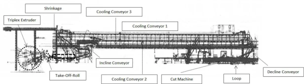
Figure 3 Extruder Composition ... 2

Figure 4 First three main components of the line after the extrusion ... 3

Figure 5 Further components of the line ... 4

Figure 6 Final divisions of the production line ... 5

Figure 7 System breakdown of the extrusion line ... 6

Figure 8 System Breakdown of the control process ... 6

Figure 9 System Breakdown of the quality control ... 6

Figure 10 System Breakdown of the maintenance syste ... 7

Figure 11 System Breakdown of the power distribution ... 7

Figure 12 Force diagram in a suspended uniform chain ... 9

Figure 13 Schematic of the cutting machine ... 11

Figure 14 Schematic of the loop ... 11

Figure 15 Inputs and outputs of the system ... 12

Figure 16 Location of the different zones of the extrusion line ... 13

Figure 17 Metering Screw... 14

Figure 18 Extruder screw with constant lead and diameter ... 14

Figure 19 Curve of the material on the loop ... 16

Figure 20 Loop Simulation ... 17

Figure 21 d-q axis representation retired from [6]. ... 22

xvi

from [7] ... 24

Figure 25 Pulse Width Modulation edited from [11] ... 26

Figure 26 Harmonics edited from [11] ... 27

Figure 27 Block scheme of the PWM simulation ... 27

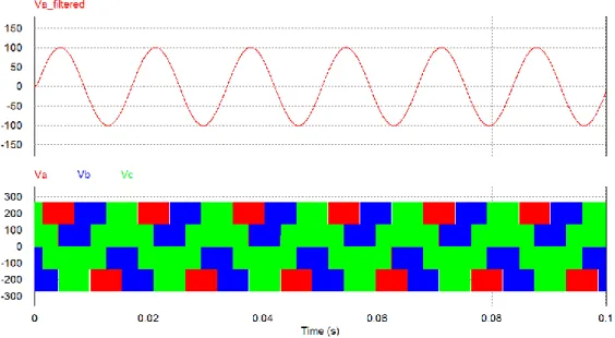
Figure 28 Top plot fundamental harmonic of the generated voltage and in bottom plot three-phase voltages. ... 28

Figure 29 FFT of the fundamental harmonic of the generated voltage and in bottom plot three-phase voltages. ... 28

Figure 30 Reference vector approximation edited from [8] ... 29

Figure 31 Space vector diagram retired from [8] ... 30

Figure 32 Seven segment SVM scheme with two passive vectors ... 30

Figure 33 SVM simulation block scheme ... 31

Figure 34 Top plot fundamental harmonic of the generated voltage and in bottom plot three-phase voltages with SVM ... 31

Figure 35 FFT of the signals presented in the figure 31 ... 32

Figure 36 FOC scheme retired from [8] ... 33

Figure 37 Direct Torque Controller with hysteresis, edited from[14] ... 34

Figure 38 Direct Torque Controller scheme, edited from [17] ... 35

Figure 39 Flux diagram, edited from [7] ... 35

Figure 40 Predictive controller, edited from [17] ... 36

Figure 41 DTC simulation block scheme ... 37

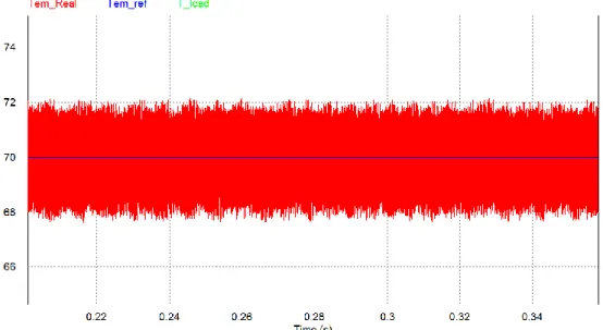
Figure 42 Torque response of the DTC with SVM ... 38

Figure 43 Torque ripple of DTC with SVM simulation result ... 39

Figure 44 Settling time of DTC-SVM simulation result ... 39

Figure 45Stator flux simulation result ... 40

Figure 46 Torque response with DTC-SPWM simulation result ... 40

Figure 47 Torque ripple of DTC with SPWM simulation result ... 41

Figure 48 Settling time of DTC-SPWM simulation result ... 41

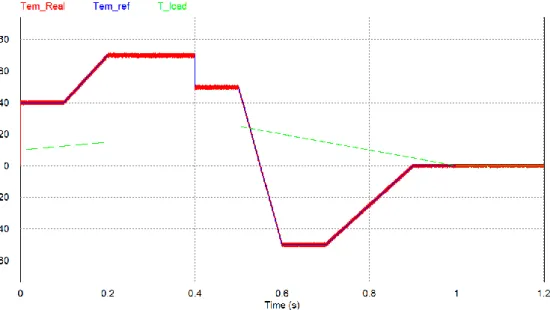
Figure 49 Simulink block scheme for simulation of the mechanical model controlled by the LQR ... 45

xvii

Figure 50 Simulation Results for and reference with a load of 10Nm. In the

first picture is simulated the position control and in the second the speed control. ... 46

Figure 51 Position control block scheme implemented in PSIM ... 46

Figure 52 Position control simulation results for a position reference of 10 rad. ... 47

Figure 53 Speed control with LQR for a speed reference of 10 rad/s ... 47

Figure 54 Position control with load compensation ... 48

Figure 55 Position control without load compensation ... 48

Figure 56 Simulink block scheme in order to get offline data to simulate the EKF in the Matlab script ... 53

Figure 57 Load estimation results from the Matlab script for an real load of 10Nm ... 53

Figure 58 Estimation results of the EKF in PSIM ... 54

Figure 59 Position control with load compensation ... 54

Figure 60 Speed control with load compensation ... 55

Figure 61 Introduction of the optimal controller in the simulation block scheme ... 58

Figure 62 Simulation results of the optimal position control ... 59

Figure 63 XMC4500 hardware applications example ... 62

Figure 64 Current conditioning circuit simulation ... 64

Figure 65 Simulation results of the conditioning current circuit. The blue signal is the voltage in the precision resistance, the red signal the output of the conditioning circuit. ... 65

Figure 66 Implementation results of the conditioning current circuit. The yellow signal is the voltage in the precision resistance, the blue signal the output of the conditioning circuit and finally the red signal the subtraction of the blue signal with the yellow. .... 65

Figure 67 Integrated circuit for voltage level conversion ... 66

Figure 68 Implementation results of the voltage level conversion circuit ... 67

Figure 69 Encoder signals, retired from DAVE help software ... 67

Figure 70 Determination of the zero position of the motor. In orange the back electromotive force and in blue the Index signal from the encoder. ... 68

Figure 71 Zero crossing of the compound back electromotive force and the Index pulse. ... 69

Figure 72 PWM signal generated by the microcontroller ... 69

Figure 73 Dead time of the generated PWM signal ... 70

Figure 74 Function diagram and truth table of HCF4053B ... 72

Figure 75 Oscilloscope results of the PWM voltage level conversion. On yellow it can be seen the input signal and on blue the output signal. ... 73

xviii

Figure 77 TDM used in the microcontroller ... 76

Figure 78 Final hardware applications structure ... 76

Figure 79 ADC block scheme simulation ... 77

Figure 80 Final simulation of the control position including the implementation conditions .. 78

Figure 81 Torque ripple when then implementation conditions are included ... 78

Figure 82 Generated phase voltage when then implementation conditions are included ... 79

Figure 83 Simulation results with the improved DTC scheme and considering the implementation conditions ... 80

Figure 84 Torque ripple with the improved DTC scheme and considering the implementation conditions ... 80

Figure 85 Generated phase voltage with the improved DTC scheme and considering the implementation conditions ... 81

Figure 86 Material inside the loop using the new transport algorithm ... 82

Figure 87 Comparison of the number of the produced treads with both transport algorithm . 83 Figure 88 Final control design ... 86

Figure 89 Implementation of the final circuit ... 87

Figure 90 Mechanical dimensions of the designed mechanical support ... 91

Figure 91 Frontal support for the encoder connection ... 92

xix

List of Tables

Table 1.1 Document Structure ... 1

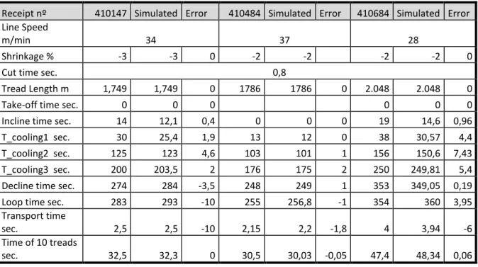
Table 2 Comparison of simulation data with real data from the production line ... 19

Table 3 Simulation Parameters ... 27

Table 4 Simulation parameters of SVM ... 31

Table 5 Motor Parameters ... 37

Table 6 Hardware applications of the microcontroller ... 63

Table 7 IGBT main characteristics ... 71

Table 8 Drivers main characteristics ... 71

Table 9 Truth table of HCF4053B ... 72

Table 10 Function running time of XMC4500 ... 75

xx

Abbreviations (alphabetical order)

AC Alternating Current

ADC Analog-to-Digital Converter

CAN Campus Area Network

CMSIS Cortex Microcontroller Software Interface Standard

DAC Digital-to-Analog Converter

DC Direct Current

DSD Delta Sigma Demodulator

DSP Digital Signal Processor

DTC Direct Torque Control

EKF Extended Kalman Filter

FEUP Faculty of Engineering of the University of Porto

FFT Fast Fourier Transform

FOC Field Oriented Control

FPGA Field Programmable Gate Array

HMI Human Machine Interface

IGBT Insulated Gate Bipolar Transistor

LQR Linear Quadratic Regulator

LSB Least Significant Bit

MCU Micro Controller Unit

MIMO Multiple Input Multiple Output

MIMO Multiple Input Multiple Output

MISO Multiple Input Single Output

MPC Model Predictive Control

MSc Master of Science

PFC Power Factor Correction

PI Proportional Integrative

PID Proportional Integrative Derivative

xxi

PWM Pulse Width Modulation

RMS Root Mean Square

RPM Rotation Per Minute

S.A. Sociedade Anónima

SPWM Sinusoidal Pulse Width Modulation

SVM Space Vector Modulation

TCU Temperature Control Unit

TDM Time Division Multiplexing

TUE Total Unadjusted Error

Symbols List

Tension on the material

Horizontal tension on the material

Derivative operator

Linear Density

Half-length of the chain

Laplace transform

( ) Tread Length at instant k

Input speed

Output speed

Time step

Relax Constant

Cooling Constant

Length of the Zone

Line Speed

Cut Time

Take-Off-Roll zone length

( ) Length of the material inside the Take-Off-Roll zone at instant k

Shrinkage zone speed

Shrinkage zone length

( ) Length of the material inside the Shrinkage zone at instant k

Incline zone length

( ) Length of the material inside the Incline zone at instant k

Incline zone speed

( ) Length of the material inside the Cooling zone 1 at instant k

Cooling zone 1 length

Cooling zone speed

( ) Length of the material inside the Cooling zone 1 at instant k ( ) Length of the material inside the Cooling zone 2 at instant k

xxii

Cooling zone 3 length

( ) Length of the material inside the decline zone at instant k

Decline zone length

Decline zone speed

( ) Length of the material inside the loop zone at instant k

Loop zone length

Transport conveyor speed

Minimum distance of the catenary to the floor

Rotor Electric Angular Speed Rotor angular speed

Number of Poles

u, v and w phase currents

-axis current component -axis current component Rotor Electric Position Stator Voltage

Direct-axis stator voltage Quadrature-axis stator voltage Stator phase resistance Stator current vector Air-gap flux vector

Quadrature-axis flux component Direct-axis flux component

Permanent magnet flux

Direct-axis inductance Quadrature-axis inductance Electromagnetic torque Moment of Inertia Friction coefficient Load torque

Amplitude of the control signal

Amplitude of the triangular wave

Amplitude modulation index Frequency modulation index

Frequency of the control signal

Bus-DC voltage

xxiii

Torque angle increment

Cost function

Solution of the Ricatti equation

Process noise Observation noise

Process noise covariance matrix Observation noise covariance matrix Innovation covariance matrix Kalman gain

Observation matrix

Initial rotor speed Initial rotor position

Torque brake

Carrier signal frequency

Fixed reference frame

d-q Rotating reference frame

a,b,c phase voltage

Voltage vector reference

Voltage angle in reference frame

Stator flux position

Torque angle

Reference flux stator amplitude

Control angle

-axis voltage reference

-axis voltage reference

State vector Input vector Observation vector

( ) State estimation function

( ) Measurement estimation function

Jacobian process matrix Jacobian observation matrix

Estimated process covariance matrix

Corrected process covariance matrix

Observation error

Predicted/Estimated state vector

Corrected state vector

Estimation state matrix

xxiv

LQR gain

Q Process cost matrix

R Output cost matrix

Output matrix

Feedforward matrix

Input disturbance

Output disturbance

Stop time

Rotation speed of the simple extruder of 200mm of diameter in rpm

Rotation speed of the simple extruder of 150mm of diameter in rpm

Rotation speed of the simple extruder of 90mm of diameter in rpm

Average perimeter

Average diameter

Screw diameter

Interior screw diameter

Area of the normal section

Interior distance of the lead

Outside distance of the lead

Height of the normal section

Volume of the lead

Chapter 1

Introduction

1.1. The Project

This Dissertation is related to the internship in Continental Mabor within the ContiMaster prize, offered to the best student that finish the 4th _{year of the Master in Chemical,}

Industrial, Mechanics and Electronic Engineering, being developed in the Faculty of Engineering of the University of Porto (FEUP), within the MSc in Electrical and Computer Engineering providing the opportunity to develop a final project in the faculty.

The initial propose of the internship was to do the dissertation in the ambit of the project, “Upgrade of the Extrusion Line”, which had as principal objectives the knowledge about the extrusion process and systems related to it, a survey of the actual electronic and mechanical components of the line and finally from the comparison of different solutions offered by different enterprises the choice of the new components.

However with the knowledge of the process and the real working conditions, was identified an high variation on the cutting length in the actual cutting system, not only related to the actual mechanical conditions that can be improved, but also the algorithm used to move the tread material to the cut position, leading with material out of tolerance.

In this way was proposed to develop a new drive system, using the position of the material as control variable and not the line speed of production as it is the actual system. The new drive system should be based in the state of art of the motors control, with the application of the most modern control techniques and using a low-cost microcontroller. Despite the technological upgrade project was being developed during the internship and at same time were developed new solutions for other projects, as for example a new programming algorithm for tread detection using Siemens Step 7, they are outside of the ambit of this Dissertation, being all this document about the development of a new algorithm to control the final position of the material in the cutting system.

1.2. Company Presentation

1.2.1. The Company: Continental AG

In October 8 of 1871 Continental-Caoutchouc- und Gutta-Percha Compagnie is founded in Hanover as a joint stock company. Manufacturing at the main factory in Vahrenwalder Street includes soft rubber products, rubberized fabrics, solid tires for carriages and bicycles.

Later in 1892 Continental is the first German company to manufacture pneumatic tires for bicycles and in 1898 has started the production of automobile pneumatic tires without tread pattern starts in Hanover-Vahrenwald.

But the big step was coming and in 1904 Continental presents the world's first automobile tire with a patterned tread.

In 2001, Continental acquired the DaimlerChryler’s automotive electronics which is now part of the Continental Automotive systems. Later in 2004 Phoenix AG joined also the group and in 2006 the automotive electronics unit of Motorola in 2006.

In 2007 Continental acquires Siemens VDO Automotive AG and advances to among the top five suppliers in the automotive industry worldwide, at the same time boosting its market position in Europe, North America and Asia. Continental is structured in six divisions:

 Chassis & Safety

 Powertrain

 Interior

 Passenger car & Light Truck Tires

 Commercial Vehicle Tires

 ContiTech

The group is specialist in the production of breaking systems, dynamic vehicle control, power transmission technologies, electronic systems and sensors. Continental has approximately 150 000 collaborators, divided between 36 countries in about 200 different locations.

1.2.2. Continental Mabor

A joint venture is set up together with the Portuguese company Mabor for the production of tires in Lousado in 1989/1990. 1993 sees complete takeover of the tire activities and of a factory producing textile cord.

Mabor stands for "Manufatura Nacional de Borracha" and was the first factory of pneumatics in Portugal. It started its process in 1946 with the assistance of General Tire.

In July of 1999, it started a great restructuration program that transformed all the old installations of Mabor in the one of the most modern 21 units from Continental. Starting from a 5000 tires a day production, it developed to 21 000 in 1996. Currently Continental - Mabor has the capacity of an average of 44 000 tires a day therefore being one of the factories with better productivity index.

Finally in 2012 Mabor receives the Quality Prize of the Continental group, being the first producing tires for the group Porsche.

Motivation 3

Initially only producing Mabor brand tires, nowadays, the spectrum of the company is much larger not just in brand but in sizes and types. Almost all of the production is meant for exportation, and more than half of this is absorbed by the substitution market, and the rest is distributed through assembly lines.

Continental - Mabor has a total area of 204 140 square meters and about 1600 collaborators.

1.3. Motivation

Henry Ford, in 1913, was the creator of the first assembly line in series production vehicles [2]. The purpose of creating these lines was to increase production in the shortest time possible and at the lowest cost.

Thus, automated production lines represent a fundamental choice in production systems where high production volumes and constant quality assurance must be guaranteed [1].

Nowadays, the competition is not just between industries, it is also between companies of the same group, being the competition and source for continuous technological changing in order to improve and also arrive to the optimal solutions in the production.

An extrusion line is a complex and extensive system, composed by many different subsystems with many different technologies. So the technological upgrade of one extrusion line represents a big chance to meet old technologies that are present in the industry, such as automata, drives, motors, etc., and also an occasion to know the state of art of the industrial communications, automation and measurements system with high precision in the industrial environment.

Even though that from the comparison of many different solutions offered by many companies, with most recent technology is obtained the best solution, sometimes the best solutions are specially designed for the applications, reflecting advantages that general solutions presented in the market cannot achieve.

Upon analysis of the process comes to the conclusion that only the replacement of the traction system in the transport conveyor for new servo-motors and automata Siemens would just guarantee the same behaviour, obtaining in this way the same performance and precision.

Represents in this way an opportunity to develop a dedicated solution for the transport system in the cutting machine, representing an enormous opportunity to understand and learn new control techniques, power electronics, motor control, microcontrollers programming, etc. and its application in the industrial level.

Not only the domain of all these themes but also represents the chance to create a new product, with high value for the enterprise represented in the increase of the production with high quality and lower waste of the produced material. Furthermore the designed solution can also attract the interest of other companies that belong to the group with the positive results obtained in Mabor.

The proposed project aims to use new modern control methods and its application in the industry with known potential which should increase the speed and precision of the system whose domain will certainly be an asset for future projects.

1.4. Objectives

After few months of formation and work on the extrusion line, was identified a high variance in the cutting-length system, that results in high percentage of material put of tolerance and so high production costs for the enterprise. To solve that this year has started the technological upgrade of the production line, having as main objectives the reduction of the power consumption, the implementation of the PROFINET communication, reduce the cost of the maintenance and to reduce the risks of failure. Despite the technological upgrade plan for the all extrusion line, it only consists for the cutting system in replacement of the obsolete electronic components, keeping the actual cutting algorithm and mechanical structure. Besides the problem with sliding of the material, the current algorithm, which relies upon the line speed where the final position is controlled by a hysteresis controller using the mechanical brake, also adds error to the final cutting position.

In order to achieve higher precision, according with the specified tolerances of the production and also higher speed, was launched the challenge to develop a new control system of the transport conveyor.

Firstly was proposed to develop a model of the extrusion line. It is necessary to know if the actual system is already optimized in terms of the speed production or if is possible to improve it. The results should be compared with the real system to validate the model.

On the other side the developed mathematical representation of the line should be used considering the new drive system, in order to simulate the new algorithm developed and to get valid conclusions about the new control system in the line performance.

At the industrial level the implementation of a new system should always ensure the complete operation of the actual system for the case of failure the new system, so the first requirement is that the controller should be able to control the speed of the traction motor. The acceleration of the motor and deceleration should also be controlled with the objective of avoiding the sliding of the material. Finally it is meant to develop a new algorithm based in the material position being necessary to control the position of the motor.

In order to achieve the main goal of developing a new control for the transport system and the system modelling the main objectives are:

1. Modelling the extrusion line;

2. Validation of the model with the system;

3. Design the drive system using a new the control architecture; 4. Simulation of the model of the production line;

5. Simulation of the model considering the new controller for moving treads; 6. Implementation of the designed control in lab environment;

Document Structure 5

1.5. Document Structure

This document is divided in 7 chapters. Due to the nature of this project that consists in the development of a new control system which has no academic predefined structure, the presented structure will be different from the canonical form as it follows the steps that were taken during the development in order to better understand its final design and components. Each contains several subsections according to the subjects mentioned.

Chapter 2 introduces and shows an overview of extrusion process and the line components as form of framework.

Chapter 3 presents a mathematical model of the extrusion system and its validation with the real system.

Chapter 4 refers to the motor modelling, modulation methods and the fundamental component of the control system, the torque controller.

Chapter 5 revolves the position and speed controller and the development of a new optimal control scheme.

Chapter 6 reports the implementation of the controller, a modified scheme of the torque controller and finally the system validation and final simulation.

Chapter 7 presents an overview of the project; final conclusions are made as some suggestions about future possible developments.

Table 1.1 Document Structure

Chapter Title

1 Introduction

2 System Overview

3 System Modelling

4 Motor Control

5 Control of the transport conveyor

6 System Validation and

Implementation

Chapter 2

System Overview

In this chapter it is intended to summarize the processes and the components inherent to a production line fully automated, which make part of the extrusion process. A generic way without going into technical details at the process level because is not part of the framework of this dissertation. Each component of the line will be discussed in more detail later, so here it is just referred its main role in the process.

2.1. Basic Concepts

The extrusion is a fabrication technique, included in the forming operations. It consists in the moulding of a viscous thermoplastic under pressure through a die. Mechanical screws pressure the melted rubber and form a continuous charge of viscous fluid. The solidification of the extruded material is achieved by blowers, water spray or diving the material under the water. This technique is mainly used for producing continuous lengths of material with constant cross-sectional [1]. In this case the cross-section is defined by the die, as it is possible to observe in the next figure.

Figure 1 Basic Model of an Extruder

The die basically consists in the shape of the orifice, that the rubber will be forced to pass through, containing the profile of the tread.

There are three types of the extrusion line in the tire production, sidewall, tread and in some cases, a kind of combined line, since that is able for the production of both tread and sidewall. It also can be characterized as duplex, triplex or quadruplex line, depending on the number of extruders. It is also important to refer, that each extruder can have different diameter, according with surface area of the orifice, the die. The treads for tires have different structures, being composed mainly of a base, cover and one or two wings, being represented in figure 2.

Figure 2 Structure elements of the tread

As it is referred in this case the extruders are composed with more than one simple extruder, after the material passes through the die it is forced, on the extruder head, to pass through another die, that give the desired profile to the material, joining the material of each extruder.

For each type of tire, there is a different receipt and in every receipt is defined all the variables of the process, as the temperature of every component of the extruder, the speed of the motor that will pressure the rubber, the pressure for each extruder, etc.

2.2. Description of the production process

The E03 extrusion line that will be the main topic of this dissertation is a triplex extrusion line. So it is composed for a 90mm, 150mm and 200mm extruder. It is also a combined line because it is prepared to produce treads and side-wall, although it is mainly used for tread production.

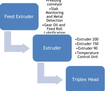
Figure 3 Extruder Composition

Feed Extruder •Feeding conveyor •Slab Monitoring and Metal Detection •Gear Oil and

Feed Roll Lubrification Extruder •Extruder 200 •Extruder 150 •Extruder 90 •Temperature Control Unit Triplex Head •Triplex Head Control (RMEA and IPOC) •Cassette

Description of the production process 9

The process begins with the compound feeding of the extruder process. Each feeder is composed principally by a feeding conveyor and a metal detector. The rubber can contain metal pieces, which represents a high hazard to the extruder. It can damage seriously the screw, that would represent the stop of the line for a long time and so a high cost to the enterprise.

Specifically for the E03 extrusion line the produced treads for tires are composed of a wing, a base and cover, existing one extruder for each component. That is why in the case of the E03 extrusion line there is a triplex extruder.

Each part of the extruder must have a temperature defined by the receipt which is guaranteed by Temperature Control Unit (TCU).

In the triplex head the screw pushes the material to pass through the die, getting the desired profile. It is important to refer, that the screw speed is controlled by RMEA. It basically consists in a fuzzy logic system that according to the weight per length and width defined in recipe it accelerates or decelerates the screw. Beyond to control the rotation speed of each extruder, it also controls the line speed value, ensuring the continuous flow of the material from the extruders to the line. There is also another control system named IPOC, belonging to the structure of the RMEA and that indicates to the operator when one recipe is finish and he can start with the production of the next recipe. The main function of this program is to avoid the mixture of different compounds inside the extruder for different recipes.

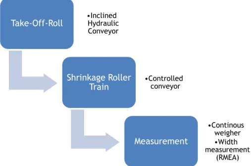
Figure 4 First three main components of the line after the extrusion

The material flows continuously from the triplex head and is retracted by the take-off-roll, starting its long path along the process. It should avoid that the material expands or shrink in next phases, it is necessary to eliminate all the tensions that exist inside the material. That is why after the material is retracted. There is a group of cylinders, rolling with different angular speed to relax and eliminate all tensions inside the material. This is the shrinkage roller train.

The speeds of all the conveyors situated after the take-off-roll are controlled using mechanical dancers. This dancer measure the existing tension on the material between two conveyor, increasing or decreasing the speed of the next conveyor, avoiding the break or the stock of material in some positions of the line.

Take-Off-Roll

Shrinkage Roller

Train

Measurement

To control the head of the extruder, and verify the properties, it is necessary to measure online the weight per length and the width. The width is measured resorting from the image processing of the RMEA system and through the weight per length using a continuous balance.

Figure 5 Further components of the line

Consequently, the material needs to be identified with a marking device. The marking process basically consists in a continuous paint of lines with different colours. The number of lines and its colours consists in a code that will identify later the recipe of that material, existing installed one vision system that checks the right colour and position of the stripes, considering the material out of tolerance if the stripes are not correct. There is also a printing device, consisting in a laser jet that prints a reference on the surface of the material as its flowing.

The next step is the solidification of the material. So, the material is moved to the superior level of the extrusion line, where are situated the water tanks. The tread flow is bathed in water, moving underwater during three paths of water tanks. In the end, to remove the water from the material, there are a series of blowers and, after it, the material goes down again to the cutting machine.

The cutting process is composed by the loop and the cutting machine. The cutting machine has a transport conveyor and a transversal motor with the knife for cut. During the cut the material is stopped in the transport conveyor and before that the line continues to produce material. So the loop, situated before the transport conveyor has the function to accumulate material while the tread is cut. After the cut, the transport conveyor has to move more material to the cut position removing material from the loop.

Marking Device

Cooling tread

Cutting tread

Description of the production process 11

Figure 6 Final divisions of the production line

To conclude, it is important to retain that it must be checked the length, the width and the continuous weight to ensure the material features defined in the recipe. If the measurements are inside the range of the tolerance values, the material is accelerated and retracted by an automatic system, the booking roller train. If is not, the booking does not retract the material and it will follow till be removed by an operator. The material that is not in good condition can still be reutilized and it is still used again in the mixing process.

2.3. System breakdown

A system breakdown is a structuring method based on system and product decompositions, creating a system architecture for better analysis and understanding [2].

Because all the production line represents a very complex and extensive system, to understand all involved components it is presented a system breakdown structure of all this process.

In a first approach, of all system, the whole system can be divided in three principle components:

 The mechanical process as the transport, cutting process;  The control of the process;

 The power systems.

Check

Dimensions

Acceleration

Figure 7 System breakdown of the extrusion line

At the second level and at the control process level, there are since the drivers to the motors, the automatons, the interfaces for the user until the communication system.

Figure 8 System Breakdown of the control process

In quality guarantee field, there is since the metal detection on the feeder extruder till the measurement system, which checks if all the dimensions and profiles of the product are in agreement with the recipe that is being produced at that moment.

Figure 9 System Breakdown of the quality control

Extrusion Line Line Conveyor Electric Motors DC Motor AC motor Servomotor Marking Device Videojet

Water Tanks Cutting

Machine Extruder Booking

Shrinkage Roller Train Process Quality Control Control Process Maintenance Systems Power systems Power Distribution Emergency Circuits Electric motors Converters Control Process Drives AC/AC Simovert Micromaster 420 AC/DC Simoreg Starters Servo-drives PLC Step 5 User Interface Switching on

the line Main Panel

Keyboard Printer Monitor Panel at the end of line Keyboard Monitor Line Network I/O Profibus BCD RMEA IPOC Quality Control Measurement systems Weight Control Continuous weigher Check weigher

Profile Control Width measurement RMEA Length measurement Slab Monitoring and Metal Detection

System breakdown 13

Finally, the maintenance system is responsible for all mechanical lubrication, control temperature, etc. On the other hand there is the power system responsible for all power distribution as represented in the figure 10 and 11.

Figure 10 System Breakdown of the maintenance system

Figure 11 System Breakdown of the power distribution

Maintenance System Refrigerating Systems TCU Tempering Extruder Tempering Triplex head Tempering Cassettes Lubrification Systems

Gear and Feed Roll Lubrification Central Grease Lubrification Power Distribution High Voltage Feeding Voltages Drives Auxiliar voltages DC-AC Converter 230V 50HZ Control Voltages DC/DC Converter to 24V Ground System

Chapter 3

System Modelling

3.1. Introduction

In order to analyse the actual performance of extrusion line, to find what is the bottleneck and what should be done to increase the speed production, is developed a mathematical model to simulate the actual state of operation. With a good model will be possible to also evaluate its performance and stability if some change is done in order to increase the speed of the production. So in this chapter each division of the production line will be modelled, being used data obtained from the normal operation of the line to validate the model. In this way can be found a simplified model of the extruder, of the each division of the line and finally of the cut system.

3.2. The catenary equation

The natural curve that a suspended chain supported only at its ends takes in the space is represented by the catenary equation 3.2.5. It was first studied by Robert Hooke in 1670 and this equation was developed by Leibniz, Huygens and Johann Bernoulli in 1691.

Assuming a uniform chain with linear density in a uniform gravitational field, the weight is about uniformly distributed.

Figure 12 Force diagram in a suspended uniform chain

Where represents the tension on the material, the horizontal component of the tension cause by the weight of the material and the half-length of the chain.

Consider the equilibrium of an infinitesimal length of chain, in a reference frame, we have

(3.2.1)

and that,

From this we get the differential equation for the curve:

√ (3.2.3)

This is a separable first order equation in respect to . Integrating in order to and defining it results

(3.2.4)

Integrating a second time it gives:

(3.2.5)

This is the catenary curve. In order to the geometrical parameters of the chain we have that √ ⇔ √ (3.2.6)

Applying a simple integration in order to it gives

(3.2.7)

3.3. The cutting tread system

Before to explain the cutting system it is important to understand what is the Loop and the main rule in the cutting system.

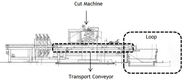
When the material is stopped to begin the cut of the tread, all the flow of material before the cutting system cannot be stopped in order to guarantee a continuous production. So the material was accumulated in the Loop. There is on the Loop an open space between the decline conveyor and the transport conveyor of the cutting system. The material is accumulated here and because it is suspended in the extremes of both conveyors making a catenary curve, as represented in the next picture.

The cutting tread system 17

Figure 13 Schematic of the cutting machine

Now it is possible to explain the actual algorithm of the control system. There are two main phases:

1. The transport phase: in this phase the material is moved until the length after the blade is smaller than the desired cut-length;

2. The cut phase: when the transport conveyor is stopped in order to cut the material with a blade. In this phase the material is accumulated in the Loop.

During the transport phase, the transport conveyor has two defined speeds according with the position of the material in the loop.

According with the figure 14, if the material is under the position h1 there is enough accumulated material on the Loop. So the transport conveyor speed is 1.5 times faster than the speed of the decline conveyor.

If the material is above the position h1 the transport conveyor speed is the same as the

decline conveyor in order to keep on the continuous flow of the material. Otherwise the material would be tensioned and the continuous chain of material would break. If the material passes through the position h2 the line stops because there is too much material in the Loop and the cut-machine is not faster enough to answer to all this debit of material.

Figure 14 Schematic of the loop

When the length of the material after the blade is near of the desired length value it is applied a mechanical brake to stop the material transport. The instant when the mechanical brake is applied is adjusted according with the average error of the cutting length. If the material is too long the mechanical brake will be applied in advance. Otherwise, if it is too short it will be applied delayed.

3.3.1. Problem Identification

The actual cutting system is the main problem present in all the extrusion lines. There is a big variance present in the cutting length which leads to a high number of rejected treads. So it is necessary to produce a higher total number of treads in order to get the desired number of good treads. This leads to the increase the costs of production and an efficiency reducing.

There are mechanical problems in the cutting machine such as:  Drift of the material during the brake;

 The error introduced by the gear-box resolution;  Variable time delay for breaking;

The variable time delay will introduce variations in the final position of the tread. On other hand the movement system is a speed controller and does not have in account the position of the tread. So when the tread is arriving at the final position it is applied the full brake, which sometimes can exceed the maximum friction introducing overshoot in the final position. As a result of this overshoot, the motor is not able to come back and the final position will be wrong, then cutting length of the material.

This problem can be solved if:

 The maximum applied brake is dimensioned according with the maximum friction;  If the controller is a position controller without overshoot the desired position

instead of the speed controller;

 The position controller has a low approach speed;

 The brake is applied by the motor, reducing the variance in the time brake;  If the intensity of the brake could be controlled.

All this aspects will be taken in account during the development of new control system for the transport conveyor.

3.4. Mathematical model of the production line

The production of treads for tires trough extrusion is a continuous production process. The system can be modelled as a Multiple Input Single Output (MISO) system, where the inputs are the RPMs of each extruder and the output the number of treads, as represented in the next picture.

Figure 15 Inputs and outputs of the system

First it is important to refer that on the topological level the production line is represented as a continuous flow of material that reaches different zones of the line while the conveyors are moving. On the picture below is presented the topological structure of the actual extrusion line and it is identified each zone.

Mathematical model of the production line 19

Figure 16 Location of the different zones of the extrusion line

On the other side this system exhibits both continuous and discrete dynamic behaviour, representing the continuous flow of the material the continuous behaviour and the cut-machine the discrete.

The main question that appeared during the development of this model was which variable should be used in order to represent the tread? Should it be the volume, the height or the length? Once is the length of material present in the loop that defines the minimum height and so the speed of the transport conveyor, is the length of the material that defines the quantity of material present in the line and finally because what defines the cycle time of the cut machine is the length of each piece, the variable that will be used to model the system is the length in meters.

3.4.1. Extruder Model

The materials used for tread production are thermoplastic, meaning that can be deformed with the increase of the temperature. In this way is it used the hot extrusion process as the process for moulding the material with the desired shape. As referred before usually for tread production the extruders are composed with more than one simple extruder, being the material of each extruder forced in the extruder head to pass through a die, giving origin to the final structure of the tire tread.

The main objective of this model is to determine the rotation speed that each extruder should rotate in order to secure the continuous flow of the material according to the defined line speed of the product that has been produced and from that analyse how the actual structure of extruders limit the production speed.

The developed mathematical model consider that in steady state, and neglecting all the dynamics effects of the rubber, that each extruder is independent of the other existing one function which relates the rotation speed of each extruder to the material debit to the line, as presented in equation 3.4.1.1. In this way the equations developed consider a single extruder with single screw to be modelled.

[ ] ( ) (3.4.1.1) The screw in the fundamental component of the extruder, being the quality and capacity of production of the extruder related to its design. The extruder is divided in three sections or barrel zones: feeding, mixing and metering section, identified in the next picture.

Figure 17 Metering Screw

The compounds are inserted in the feed section that with the screw rotation will flow inside the extruder. In the mixing section the pressure and the high temperature gives origin to a uniform melt, being possible, in this zone, to insert pins on the barrel to achieve a more homogenous melt.

The main idea of the model is to determine the debit of the extruder, volume per second, assuming that the material inside the extruder is already compressed and will not suffer volume changes during its displacement along the screw. Every rotation of the screw results in a volume displacement of material equivalent to the volume of one lead, because it is being modelled a screw with constant lead. The mechanical draw of the screw from an extruder of 150mm can be found in appendix II and generic model of the screw with constant lead and diameter is presented in picture 18.

Figure 18 Extruder screw with constant lead and diameter

The average rotation perimeter and diameter are given by the followed expressions respectively.

(3.4.1.2)

Mathematical model of the production line 21

The area of the normal section with free space is given in equation 3.4.1.4.

( ) ( ) _(3.4.1.4) Finally the height of this section in presented in equation 3.4.1.5 and the volume in 3.4.1.6 which results from the product of the nominal section area with the height of this section.

√ (3.4.1.5)

(3.4.1.6)

The debit of the extruder is defined as the product of the rotation speed with the volume of the lead, being the speed of the material the quotient of the debit with the area of the die where the material is extruded, as presented in equations 3.4.1.7.

(3.4.1.7) This means that, neglecting the dynamic effects of the rubber, in steady state, the speed of the material is proportional to one constant, function of the dimensions of the single extruder, defined as the volume of the lead. On the other hand is proportional and inversely proportional of two variables, the rotation speed of the screw and the area of the die respectively.

Actually, the rotation speed defined in the production parameters of each receipt is obtained by experience of the operator and with several tests until the produced material has the desired characteristics. This model can be used to determine an approximation of the speeds values, simplifying the process. On the other side it can also be used for better parameterization of the IPOC program.

Although the application and precision of this model is limited since it just consider the mechanical dimensions of the extruder and die, and do not consider the dynamics effects of the rubber, which in same aspects can take relevance.

3.4.2. The line model

Each system will be modelled as a flux of material, where the material comes in and out with a defined speed. During the development of the production line model it is considered that the extruders are able produce the necessary debit of material, in order to guarantee the continuous flow of material according with the line speed. When the total length of the material reaches the length of the zone, the exceeded length should be added to the next zone ensuring a continuous flow of material. This flux is modelled with the speed in which the material comes in and out of each zone of the line. In this model it is assumed that the extruder are have to the necessary debit of material according to the line speed and ensuring the continuous flow of material.

Having ( ) as the tread length present in each zone at the instant , at the next instant the length will be

( ) ( ) ( ) (3.4.2.1)

where and are the input and output of the material speed in each zone, respectively.

One important fact is that on the shrinkage zone and in the cooling, the input speed is slower than the output of the zone before. This happens because, as it was explained before, the material shrinks and so the flux of the material in terms of length is smaller. On the other hand, the material becomes denser, but this fact is not important for this model. The same happens when the rubber goes inside the cooling tank and it is cooled, the material also shrinks.

This decrease of speed are modelled with the creation of two constant: the relax constant, , and cooling constant, .

A finite state machine was used as mathematic model, representing each state a zone of the production line and the condition transitions are modelled as

( ) (3.4.2.2)

The only discrete part is after the cutting machine where the continuous flow of rubber is transformed in individual parts that will make part of the tire as final product.

Here there are two states where the tread is moving: in one with 1.5 times the line speed and in the other with the line speed. There is also another state where the tread is stopped at the blade position. In the first two states, the length of material in the loop at each time step is in the first case described by:

( ) ( ) (3.4.2.3)

In the second case is constant.

( ) ( ) ( ) ( ) (3.4.2.4)

The conditions transitions are according with the position as represented in the next picture.

Figure 19 Curve of the material on the loop

The conveyors are spaced by the distance , and because the tread is suspended in the extremes of both conveyors, the curve that it describes is defined by the catenary equation 3.4.2.5, presented below, where s is half of the total length.

(3.4.2.5)

At each infinitesimal time instant, it is possible to consider a stationary curve and the length of the tread constant in each instant. With this it is just necessary to solve the above equation at each time instant in order to get the height h that will be the transition condition. Because this is a non-linear equation and to simplify the computational cost was developed an Matlab script that calculates for each instant the minimum distance to the floor, , the corresponding tread length that is on the Loop, being the values saved on a

Mathematical model of the production line 23

vector. During the simulation it is just necessary to search on the vector the corresponding length, ( ), the corresponding minimum distance. The loop simulation is presented in the next figure.

Figure 20 Loop Simulation

As presented in the figure 20h represents the vertical distance of the catenary curve that

the material does to the floor and L the quantity of material, in meters, that is inside the loop. Observing the figure 20 there are three delimited zones: A, B, and C. In zone A the transport conveyor is stopped in order to start a transversal cut in the material, during 0.8 s. As expected because the line do not stops in order to execute the cut, the material is accumulated in the loop, so L grows proportional to the line speed and the height decreases. After the cut the transport conveyor starts to move, pushing material from the loop at one speed 1.5 times the line speed, increasing again the height and decreasing the material on the loop. Finally when the height reach 0.75 m from the floor, the transport conveyor speed is set to be equal to the line speed so the material in the loop stays constant and the same happens to the distance to the floor.

The final equations system for each zone is presented next. 1. Take-Off-Roll Model Equations

{ ( ) ( ) ( )

( ) ( ) ( ) ( )

(3.4.2.6)

2. Shrinkage Model Equations

{

( ) ( )

( ) ( ) ( ) ( ) ( ) ( ) ( )

(3.4.2.7)

{ ( ) ( ) ( ) ( ) ( ) ( ) ( ) ( ) ( ) (3.4.2.8) 4. Cooling 1 Equations { ( ) ( ) ( ) ( ) ( ) ( ) ( ) ( ) (3.4.2.9) 5. Cooling 2 Equations { ( ) ( ) ( ) ( ) ( ) ( ) ( ) ( ) (3.4.2.10) 6. Cooling 3 Equations { ( ) ( ) ( ) ( ) ( ) ( ) ( ) ( ) (3.4.2.11)

7. Decline Conveyor Equations { ( ) ( ) ( ) ( ) ( ) ( ) ( ) ( ) (3.4.2.12) 8. Loop Equations { ( ) ( ) ( ) ( ) ( ) ( ) ( ) ( ) (3.4.2.13)

9. Speed Transport Equations { (3.4.2.14)

3.4.3. Conclusion

It is possible to conclude from the equations presented above that, in order to guarantee the stability of the production, the line speed between the conveyors should be the same in the case of the material do not suffer any physical modification. If the material shrinks, the speed should be proportionally reduced by the same factor.

Finally, in the case of the cutting machine, the average flux of the transport conveyor should be the same as on the Loop to ensure that the average length of material inside the Loop is the same as the taken out by the transport conveyor.